F. A. BARTHA1, F. FODOR2, AND B. GONZALEZ MERINO3
Abstract. We prove that the volume of central hyperplane sections of a unit cube inRnor- thogonal to a main diagonal of the cube is a strictly monotonically increasing function of the dimension forn≥3. Our argument uses an integral formula that goes back to P´olya [P´ol13] (see also [Hen79] and [Bal86]) for the volume of central sections of the cube, and Laplace’s method to estimate the asymptotic behaviour of the integral. First we show that monotonicity holds starting from some specificn0. Then, using interval arithmetic (IA) and automatic differentiation (AD), we compute an explicit bound forn0, and check the remaining cases between 3 andn0 by direct computation.
1. Introduction
Let Cn = [−12,12]n be the unit cube in Rn, and for u ∈ Rn let H(u) = u⊥, the hyperplane through o orthogonal to u. We are interested in determining Voln−1(Cn∩H(u0)) in the special case whenu0= (1, . . . ,1)∈Rn is parallel to a main diagonal ofCn.
Hensley [Hen79] described a probabilistic argument, whose origin he attributed to Selberg, prov- ing that Voln−1(Cn∩H(u0)) → p
6/π as n → ∞, and he conjectured that maxuVoln−1(Cn ∩ H(u))≤√
2. This conjecture was proved by Ball [Bal86], who proved an integral formula for the volume of sections that goes back to P´olya [P´ol13], which, when specialized to the case ofH(u0), is the following:
(1) I(n) := Voln−1(Cn∩H(u0)) = 2√ n π
Z +∞
0
sint t
n dt.
It is an interesting fact that the maximum volume hyperplane section of the cube occurs when the hyperplane is orthogonal to u = (1,1,0, . . . ,0), and not for hyperplanes orthogonal to the main diagonals. The limitp
6/π for the main diagonal is slightly less than√ 2.
Date: March 2, 2021.
Key words and phrases. Cube, sections, volume.
1Supported by NKFIH KKP 129877 and EFOP-3.6.2-16-2017-00015 grants and by the grant TUDFO/47138- 1/2019-ITM of the Ministry for Innovation and Technology, Hungary.
2Supported by grant TUDFO/47138-1/2019-ITM of the Ministry for Innovation and Technology, Hungary, and by Hungarian National Research, Development and Innovation Office NKFIH grant KF129630.
3 This research is a result of the activity developed within the framework of the Programme in Support of Excellence Groups of the Regi´on de Murcia, Spain, by Fundaci´on S´eneca, Science and Technology Agency of the Regi´on de Murcia. Partially supported by Fundaci´on S´eneca project 19901/GERM/15, Spain, and by MICINN Project PGC2018-094215-B-I00 Spain.
Accepted version. The published paper appeared in International Mathematics Research Notices, Vol. 2021, No.
4, pp. 2861–2881. Link to the published version: https://dx.doi.org/10.1093/imrn/rnaa254.
1
Kerman, Ol’hava and Spektor [KOS15] proved the asymptotic expansion
(2) I(n) =
r6 π
1− 3
20n − 13 1120n2
+O(n−3),
improving the previous computation of Borwein, Borwein and Leonard [BBL10]. However, the size of the error termO(n−3) was not computed yet.
It is known that the integral (1) can be evaluated explicitly as (3) Voln−1(Cn∩H(u0)) =
√n 2n(n−1)!
n
X
i=0
(−1)i n
i
(n−2i)n−1sign(n−2i),
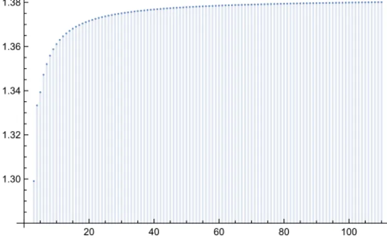
see Goddard [God45], Grimsey [Gri45], Butler [But60], and Frank and Riede [FR12]. Numerical computations with (3) suggest that Voln−1(Cn ∩H(u0)) is a strictly monotonically increasing function ofnwhile it tends to the limitp
6/πasn→ ∞. However, (3) does not seem to lend itself as a tool for proving this monotonicity property.
20 40 60 80 100
1.30 1.32 1.34 1.36 1.38
Figure 1. Voln−1(Cn∩H(u0)) for 3≤n≤110 plotted byMathematica.
Recently, K¨onig and Koldobsky proved that, in fact, Voln−1(Cn∩H)≤p
6/πfor alln≥2, see [KK19, Prop. 6(a)]. We also point out the recent result of Aliev [Ali20] (see also [Ali08]) about hyperplane sections of the cube, in which he proves that
(4)
√n
√n+ 1 ≤ I(n+ 1) I(n)
which is slightly less than the monotonicity of Voln−1(Cn∩H(u0)).
For a more detailed overview of the currently known information on sections of the cube and for further references, see, for example, the books of Berger [Ber10] and Zong [Zon06], and the papers by Ball [Bal86, Bal89], K¨onig, Koldobsky [KK19] and Ivanov, Tsiutsiurupa [IT20].
Our main result is the following.
Theorem 1. The volume Voln−1(Cn∩H(u0))is a strictly monotonically increasing function ofn for alln≥3.
Theorem 1 directly yields the following corollary (which has already been proved by K¨onig and Koldobsky [KK19]), and slightly improves the estimate (4) of Aliev mentioned above. It also computes the size of the error term in (2).
Corollary 1. For any integern≥2, it holds that
Voln−1(Cn∩H(u0))<
r6 π. and this upper bound is best possible.
The rest of the paper is organized as follows. In Section 2 we use Laplace’s method to study the behaviour of the integral (1), and prove the existence of an integer n0 with the property that Voln−1(Cn∩H(u0)) is an increasing sequence for alln≥n0. In the Appendix, using interval arithmetic, automatic differentiation, and some analytical arguments, we provide rigorous numerical estimates, which we use in Section 3 to obtain an explicit upper bound on n0. Finally, we check monotonicity for 3 ≤ n ≤ n0 by calculating the value of of Voln−1(Cn∩H(u0)) using (3), thus concluding the proof of Theorem 1.
2. Proof of the monotonicity for large n
In this section, we prove the following statement which is the most important ingredient of the proof of Theorem 1.
Theorem 2. There exists an integer n0 such that Voln−1(Cn∩H(u0))is a strictly monotonically increasing function of nfor all n≥n0.
Proof. We are going to examine the behaviour of the integral:
I(n) =2√ n π
Z +∞
0
sint t
n
dt, n≥3.
We wish to prove that there exists ann0 such thatI(n) is strictly monotonically increasing for all n≥n0.
We start the argument by restricting the domain of integration to a finite interval that contains most of the integral asn→ ∞. Ifafixed, with 1< a < π/2, then forn≥3 it holds that
2√ n π
Z +∞
a
sint t
n
dt < 2√ n π
Z +∞
a
t−ndt= 2√ n π
a−n+1 n−1 < 2
3a−n=:e1(n).
Note that the function e1(n) tends to 0 exponentially fast as n → +∞. Let a be fixed, say, a=e1/6 and define
(5) Ia(n) := 2√
n π
Z a
0
sint t
n
dt, forn≥3.
Then
|I(n)−Ia(n)|< e1(n) forn≥3.
We will use Laplace’s method to study the behaviour ofIa(n). Let us make the following change of variables
sint
t =e−x2/6, thusx= r
−6 logsint t ,
where we define the value of sint/tto be 1 att= 0. Since sint/t=e−t2/6+O(t4), the substitution above yields t'xneart= 0. Therefore,x(t) is analytic in the interval [0, a]. Note thatx(0) = 0,
and x0(t) > 0 for all t ∈ [0, a]. Thus, x(t) maps [0, a] bijectively onto [0, x(a)], and so it has an inverset(x) : [0, x(a)]→[0, a], which is also analytic in [0, x(a)] by the Lagrange Inversion Theorem because x0(t)6= 0 for t∈[0, a]. In our case, 1.211< x(a) =x(e1/6) = 1.211· · ·<1.212.
The Taylor series ofx(t) aroundt= 0 begins with the terms x=t+ t3
60+ 139t5
151200+ 83t7
1296000+. . . .
We can get the first few terms of the Taylor series expansion oft=t(x) aroundx= 0 by inverting the Taylor series ofx(t) att= 0 as follows:
t(x) =x−x3
60 − 13x5
151200+ x7
336000+. . . . Then
t0(x) = 1−x2
20− 13x4
30240+R6(x)
is the order 5 Taylor polynomial oft0(x) aroundx= 0 (observe that the degree 5 term is zero), and for the Lagrange remainder termR6(x), it holds that
R6(x) = t(7)(ξ) 6! x6
for some ξ ∈(0, x) (depending on x). Since t(x) is analytic in [0, x(a)], in particular the seventh derivative of t(x) is analytic too, and thus it is a continuous function. Then the Extreme Value Theorem yields that t(7) attains its maximum in [0, x(a)], and thus |t(7)(x)| ≤R, for someR >0 and everyx∈[0, x(a)]. Then we can use the following estimate on x∈[0, x(a)]:
(6) |R6(x)| ≤ R
6!x6, Therefore, after the change of variables, we need to evaluate
Ia(n) =2√ n π
Z x(a)
0
e−nx2/6t0(x)dx
=2√ n π
Z x(a)
0
e−nx2/6
1−x2
20− 13x4
30240 +R6(x)
dx
=2√ n π
Z x(a)
0
e−nx2/6
1−x2
20− 13x4 30240
dx
+2√ n π
Z x(a)
0
e−nx2/6R6(x)dx.
(7)
In order to calculate the above integrals we will use the central moments of the normal distribu- tion: If y=√1
2πσ2e−(x−µ)22σ2 , then for an integer p≥0 it holds that
(8) E[yp] =
(0, ifpis odd, σp(p−1)!!, ifpis even.
In our caseσ2= 3/n andp= 6. Thus, using (8) and (6), we get that 2√
n π
Z x(a)
0
e−nx2/6|R6(x)|dx≤2R√ n π6!
Z x(a)
0
e−nx2/6x6dx
<2R√ n π6!
Z +∞
0
e−nx2/6x6dx
=2R√ n π6!
33 n35!!
=9R 8π
1 n5/2
<R 2
1
n5/2 =:e2(n).
(9)
Notice also that
2√ n π
Z +∞
0
e−nx2/6
1−x2
20 − 13x4 30240
dx
= r3π
2 2√
n π
1
n1/2− 3
20n3/2 − 13 1120n5/2
= r6
π
1− 3
20n− 13 1120n2
. (10)
The complementary error function is defined as erfc(x) := 2 1
√π Z +∞
x
e−τ2dτ.
It is known that erfc(x)≤e−x2 forx≥0. Then, taking into account thatx(a)>1.211, we obtain 2√
n π
Z +∞
x(a)
e−nx2/6
1−x2
20− 13x4 30240
dx
≤ 2√ n π
Z +∞
x(a)
e−nx2/6
1−x2
20− 13x4 30240
dx
≤ 2√ n π
Z +∞
x(a)
e−nx2/6
1 + x2
20+ 13x4 30240
dx
< 2√ n π
Z +∞
1
e−nx2/6
1 + x2
20+ 13x4 30240
dx
= r6
πerfc(p n/6)
13 + 168n+ 1120n2 1120n2
+ 2e−n/6√
n117 + 1525n 10080πn2
< 5
3e−n/6=:e3(n).
(11)
Now, using the monotonicity ofe1(n), we obtain that
I(n+ 1)−I(n) ≥ (Ia(n+ 1)−e1(n+ 1))−(Ia(n) +e1(n)) ≥ Ia(n+ 1)−Ia(n)−2e1(n).
Furthermore, expressing Ia (cf. (7)) as a difference of integrals in the intervals [0,+∞) and [x(a),+∞), together with the value of the integral in [0,+∞) (10) and the bounds (9) and (11),
yields
Ia(n+ 1)≥ r6
π
1− 3
20(n+ 1) − 13 1120(n+ 1)2
−e2(n+ 1)−e3(n+ 1), and
Ia(n)≤ r6
π
1− 3
20n− 13 1120n2
+e2(n) +e3(n).
Therefore
I(n+ 1)−I(n)≥ r6
π 3
20n− 3
20(n+ 1)+ 13
1120n2 − 13 1120(n+ 1)2
−2e1(n)−e2(n)−e2(n+ 1)−e3(n)−e3(n+ 1)
>
r6 π
3
20n(n+ 1) + 13(2n+ 1) 1120n2(n+ 1)2
−4
3a−n−(e2(n) +e2(n+ 1) +e3(n) +e3(n+ 1))
>
r6 π
3 20n(n+ 1)
−4
3a−n−2e2(n)−2e3(n)
>
r6 π
3 20n(n+ 1)
−4
3a−n− R n5/2 −10
3 e−n/6
= r6
π
3 20n(n+ 1)
−14
3 e−n/6− R n5/2. (12)
Clearly, there exists ann0, such that for alln≥n0the expression (12) is strictly positive. Therefore, Voln−1(Cn∩H(u0)) is strictly monotonically increasing for n≥n0.
Thus, we have finished the proof of Theorem 2.
Remark. Figure 1 suggests that Voln−1(Cn∩H(u0)) is not only a monotonically increasing sequence but also concave, i.e., 2I(n+ 1)≥I(n) +I(n+ 2) for n≥4. We note, without giving the details, that with a similar argument as in the proof of Theorem 2, but using more terms of the Taylor expansion of t(x), one can also show that
2I(n+ 1)−I(n)−I(n+ 2)
≥2Ia(n+ 1)−Ia(n)−Ia(n+ 2)−ξ1e1(n)−ξ2e2(n)−ξ3e3(n)
≥ 3√ 3 5√
2π
1
n(n+ 1)(n+ 2)+O(n−4)−ξ1e1(n)−ξ2e2(n)−ξ3e3(n),
for someξi >0,i= 1,2,3. If we take into account sufficiently many terms of the Taylor series of t(x), then we can guarantee that each error term is of smaller order thann−3, and thus there exists a numbern1 such that the sequenceI(n) is concave for alln≥n1.
3. Proof of Theorem 1
In order to prove Theorem 1, we need an explicit upper bound on the critical numbern0. Using a combination of interval arithmetic, automatic differentiation, and some analytic methods, we can obtain a rigorous upper estimate for the seventh derivative |t(7)(x)| in x ∈ [0, x(a)]. We provide
the details of this argument in the Appendix. Here, we only quote the following upper bound (see Theorem 3 part (3)):
(13) R≤0.79461.
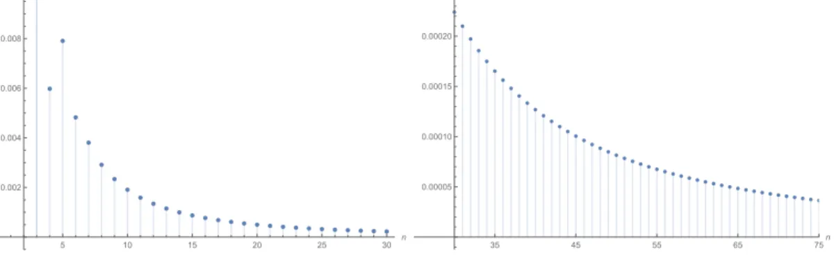
Now, substituting the estimate (13) in inequality (12), we get thatn0= 75. Then, we can calculate the values of I(n+ 1)−I(n) using (3) to the required accuracy, and verify monotonicity for all 3≤n≤75, see Figure 2 below.
0 5 10 15 20 25 30 n
0.002 0.004 0.006 0.008
35 45 55 65 75n
0.00005 0.00010 0.00015 0.00020
Figure 2. I(n+ 1)−I(n) for 3≤n≤75 plotted byMathematica Remark. Using the same ideas as above, one could show the concavity ofI(n) forn≥3.
4. Acknowledgements
We would like to thank Juan Arias de Reyna for helpful discussions and suggestions.
References
[Ali20] I. Aliev,On the volume of hyperplane sections of ad-cube, Acta Math. Hungar. (2020). https://doi.
org/10.1007/s10474-020-01057-y.
[Ali08] I. Aliev,Siegel’s Lemma and Sum-Distinct Sets, Discrete Comput. Geom.39(2008), no. 3, 59–66.
[Bal86] K. Ball,Cube slicing inRn, Proc. Amer. Math. Soc.97(1986), no. 3, 465–473.
[Bal89] K. Ball,Volumes of sections of cubes and related problems, Geometric aspects of functional analysis (1987–
88), Lecture Notes in Math., vol. 1376, Springer, Berlin, 1989, pp. 251–260.
[Ber10] M. Berger,Geometry revealed, Springer, Heidelberg, 2010. A Jacob’s ladder to modern higher geometry;
Translated from the French by Lester Senechal.
[BBL10] D. Borwein, J. M. Borwein, and I. E. Leonard,Lpnorms and the sinc function, Amer. Math. Monthly117 (2010), 528–539.
[But60] R. Butler,On the evaluation ofR∞
0 (sinmt)/tndtby the trapezoidal rule, Amer. Math. Monthly67(1960), 566–569.
[FR12] R. Frank and H. Riede,Hyperplane sections of then-dimensional cube, Amer. Math. Monthly119(2012), no. 10, 868–872.
[Hen79] D. Hensley,Slicing the cube inRnand probability (bounds for the measure of a central cube slice inRn by probability methods), Proc. Amer. Math. Soc.73(1979), no. 1, 95–100.
[God45] L. S. Goddard, LII. The accumulation of chance effects and the Gaussian frequency distribution, The London, Edinburgh, and Dublin Philosophical Magazine and Journal of Science36(1945), no. 257, 428–
433.
[Gri45] A. H. R. Grimsey,XL. On the accumulation of chance effects and the Gaussian Frequency Distribution:
To the editors of the Philosophical Magazine, The London, Edinburgh, and Dublin Philosophical Magazine and Journal of Science36(1945), no. 255, 294–295.
[IT20] G. Ivanov and I. Tsiutsiurupa,On the volume of sections of the cube, arXiv:2004.02674 (2020).
[KOS15] R. Kerman, R. Ol’hava, and S. Spektor,An asymptotically sharp form of Ball’s integral inequality, Proc.
Amer. Math. Soc.143(2015), no. 9, 3839–3846.
[KK19] H. K¨onig and A. Koldobsky,On the maximal perimeter of sections of the cube, Adv. Math.346(2019), 773–804.
[P´ol13] G. P´olya,Berechnung eines bestimmten Integrals., Math. Ann.74(1913), 204–212.
[Zon06] C. Zong,The cube: a window to convex and discrete geometry, Cambridge Tracts in Mathematics, vol. 168, Cambridge University Press, Cambridge, 2006.
Appendix Consider the function
(14) x(t) =
s
−6 log sint
t
,
where t∈[0,1.2]. The fraction sintt is understood to be augmented with its limit att = 0 that is
sin 0
0 = 1. Then, the functionx(t) is analytic.
Theorem 3. The following holds true.
(1) x(t)is strictly increasing on[0,1.2]and
x(t)≤1.231399 fort∈[0,1.2].
(2) x(t)is invertible with inverset(x), wherex∈[0, x(1.2)].
(3) The 7th derivative oft(x)attains the upper bound
t(7)(x)
≤0.79461 forx∈[0, x(1.2)].
The monotonicity stated in (1) is trivial, hence, one just needs to establish the containment x(1.2)∈[0, x(1.2)]. Note that (2) is a consequence of (1), thus, in the following we will deal with evaluatingx(t) and proving (3).
There are numerous computational steps involved. In order to obtain rigorous results, we have based our computations on two techniques, namely,interval arithmetic (IA)andautomatic differ- entiation (AD)that are capable of providing mathematically sound bounds for functions and their derivatives alike. Besides the technical hurdle, severe difficulties arise at the left endpoint t = 0 as, when computing the derivatives ofx(t), we need to differentiate both √
· and sintt at zero. It was tempting to use Taylor models, an advanced combination of these two, however that could still not handle the aforementioned left endpoint directly, hence, we chose to stick with the straightfor- ward application of the two techniques and used the CAPD package [CG20]. For a comprehensive overview of these topics we refer to [Tuc, Gri, Mak03].
We emphasize that the major goal of Theorem 3 is providing the given bounds, hence, we made little effort to obtain tighter results and were performing sub–optimal computations knowingly, in order to decrease the implementation burden.
The key step to overcome the difficulties att= 0 is to rephrase (14) as x(t) =tp
h(t),
h(t) = (g◦F2)(t)·(−6F(t)), g(t) =log(1 +t)
t ,
F2(t) =t2F(t), and F(t) =
sin(t) t −1
t2 . (15)
Section 5 details the considerations used for dealing with the functions appearing in (15). In particular, Sections 5.1 and 5.2 handle the functions sintt and F(t); a computational scheme for their derivatives is provided. Then, we turn our attention to log(1+t)t and derive analogous results in Section 5.3. The square root is discussed in Section 5.4. Then, in Section 5.5, we present a pure formula for the higher order chain–rule used to composeg(t) andF2(t). Section 6 contains the results forx(t) and its derivatives, in particular, the proof of the remaining part of (1) in Theorem 3.
Section 7 deals witht(x) by giving a general inversion procedure in Section 7.1 and the final proof in Section 7.2.
The codes performing the rigorous computational procedure described in this manuscript, to- gether with the produced outputs, are publicly available at [FAB20].
5. Bounding functions and their derivatives
First, we will closely analyze some Taylor expansions centered att0= 0 and derive bounds for Taylor coefficients of the very same functions expanded around another center point ˆt0. Then, we include the higher order chain–rule for completeness.
5.1. The function sintt. The Taylor series of sintcentered att0= 0 is given as sint=
∞
X
k=0
(−1)k t2k+1 (2k+ 1)!
and is convergent for all t∈R. Consequently, we obtain the Taylor series of f(t) :=
(sint
t , ift >0, 1, ift= 0 as
(16) f(t) =
∞
X
k=0
(−1)k t2k (2k+ 1)!,
again, centered att0= 0 with the same convergence radius. Therefore,
(17) 1
m!f(m)(t) = 1 m!
∞
X
k≥m/2
(−1)k t2k−m
(2k−m)!·(2k+ 1) form= 0,1, . . .
We shall bound these infinite series as follows. LetN ≥m/2, then, define the finite partSf(t;N, m) and the remainder partEf(t;N, m) as
Sf(t;N, m) = 1 m!
N
X
k≥m/2
(−1)k t2k−m
(2k−m)!·(2k+ 1) and Ef(t;N, m) = 1
m!
∞
X
k=N+1
(−1)k t2k−m (2k−m)!·(2k+ 1). (18)
The following lemma establishes bounds for the remainder.
Lemma 1. Let m, N∈Z withm≥0 andN ≥m/2. Then, Ef(t;N, m)∈ 1
m!
et
(2N+ 2−m)!t2N+2−m · [−1,1]
for allt≥0.
Proof. Lett≥0 and consider
|Ef(t;N, m)| ≤ 1 m!
∞
X
k=N+1
t2k−m
(2k−m)!·(2k+ 1) ≤ 1 m!
∞
X
k=N+1
t2k−m (2k−m)! ≤ 1
m!
∞
X
k=2N+2−m
tk k!. Note that we have obtained the tail of the Taylor series of the exponential function centered at t0= 0. The corresponding Lagrange remainder gives us that for all integersK≥0
∞
X
k=K
tk k! = 1
K!
dKet dtK (ξ)·tK
holds with some ξ =ξ(K)∈ [0, t]. Observe that ddtKKet(ξ) = eξ and that attains its maximum at ξ=t overξ∈[0, t]. Hence, we obtain
∞
X
k=K
tk k! ≤ 1
K!et·tK fort≥0.
Finally, setting K = 2N + 2−m and deriving a bound on Ef(t;N, m) from the estimate for
|Ef(t;N, m)| concludes the proof.
Defining
(19) Ef(t;N, m) = 1
m!
et
(2N+ 2−m)!t2N+2−m · [−1,1]
together with (17), (18), and Lemma 1 gives a rigorous computational scheme for f(t) and its derivatives, namely,
1
m!f(m)(t)∈Sf(t;N, m) +Ef(t;N, m).
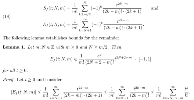
We remark that limN→∞Ef(t;N, m)→ {0} for allt∈Randm≥0. Figure 3 gives an insight on how the obtained bound for the remainder behaves.
0.2 0.4 0.6 0.8 1.0 1.2 1e-90
1e-40 1e-10
1 1.1 1.2
1e-40 1e-20
1e-8 Ef(t, 5, 0)
Ef(t, 10, 0) Ef(t, 15, 0) Ef(t, 20, 0)
0.2 0.4 0.6 0.8 1.0 1.2
1e-90 1e-40 1e-10
1 1.1 1.2
1e-40 1e-20
1e-8 Ef(t, 5, 1)
Ef(t, 10, 1) Ef(t, 15, 1) Ef(t, 20, 1)
0.2 0.4 0.6 0.8 1.0 1.2
1e-90 1e-40 1e-10
1 1.1 1.2
1e-40 1e-20
1e-6 Ef(t, 5, 4)
Ef(t, 10, 4) Ef(t, 15, 4) Ef(t, 20, 4)
0.2 0.4 0.6 0.8 1.0 1.2
1e-90 1e-40 1e-10
1 1.1 1.2
1e-40 1e-20
1e-5 Ef(t, 5, 7)
Ef(t, 10, 7) Ef(t, 15, 7) Ef(t, 20, 7)
Figure 3. The upper bound ofEf(t;N, m) for various (N, m) overt∈[0,1.2].
5.2. The function 1 +t2F(t) = sintt. Even though there are no issues with directly computing log (f(t)) using the results above, as shown in (15), we will need a more sophisticated approach in order to be able to tackle the final square root operation in the neighbourhood of zero. To that end, we rewrite expansion (16) as
f(t) = 1 +t2F(t) = 1 +t2
∞
X
k=0
(−1)k+1 t2k (2k+ 3)!,
a 2nd–order Taylor model. Analogous arguments, as in Section 5.1, lead to the following.
Lemma 2.
1
m!F(m)(t)∈SF(t;N, m) +EF(t;N, m),
where
SF(t;N, m) = 1 m!
N
X
k≥m/2
(−1)k+1 t2k−m
(2k−m)!·(2k+ 1)(2k+ 2)(2k+ 3) and EF(t;N, m) =Ef(t;N, m).
Note that the remainder bound is identical to the one in (19) as the factor in the denominator (2k+ 1)(2k+ 2)(2k+ 3) may be eliminated the same way as (2k+ 1) in the proof of Lemma 1.
5.3. The function log(1+t)t . Following (15), we will computex(t) using the form x(t) =t
s
−6F(t)log (1 +t2F(t)) t2F(t) .
Thus, the next step is to analyzeg(t) = log(1+t)t , where t∈(−1,1). This interval comes from the well-known expansion of log(1 +t). Att= 0, we augment with the limit g(0) := 1. Note that the argument ofg(·) will bet2F(t) = sintt −1 that takes values roughly in [−0.223,0].
Let us start from the Taylor series of log(1 +t) centered at t0= 0, namely, log(1 +t) =
∞
X
k=1
(−1)k+1tk k that is convergent for|t|<1. Then, formally,
g(t) =
∞
X
k=0
(−1)k tk k+ 1 and
1
m!g(m)(t) = 1 m!(−1)m
∞
X
k=0
(−1)k tk k+m+ 1
(k+m)!
k! form= 0,1, . . . that can be simplified as
1
m!g(m)(t) = (−1)m
∞
X
k=0
(−1)k
k+m m
tk k+m+ 1. We define
Sg(t;N, m) = (−1)m
N
X
k=0
(−1)k
k+m m
tk
k+m+ 1 and Eg(t;N, m) = (−1)m
∞
X
k=N+1
(−1)k
k+m m
tk k+m+ 1 (20)
for N ≥0 (practicallyN ≥mso that k+m > 2m in the binomial coefficients in Eg). We may bound the remainder part as detailed below.
Lemma 3. Let N ≥m≥0 andt∈(−1,1). Then,
|Eg(t;N, m)| ≤
( |t|N+1
(1−|t|)N+2, if m= 0,
2e m
m
m! m+Nm+1 |t|N+1
(1−|t|)m+N+2, else.
Proof. Whenm= 0, the binomial coefficient k+mm
= 1, thus,
|Eg(t;N,0)| ≤
∞
X
k=N+1
|t|k k+ 1 ≤
∞
X
k=N+1
|t|k.
On the other hand, form >0, it is known that k+m
m
≤
e(k+m) m
m . Hence,
|Eg(t;N, m)| ≤
∞
X
k=N+1
e(k+m) m
m |t|k k+m+ 1 ≤
∞
X
k=N+1
e(1 +mk) m
m km|t|k k+m+ 1 ≤
2e m
m ∞
X
k=N+1
km|t|k.
Thus, for both cases, it is sufficient to bound the series
∞
X
k=N+1
km|t|k
for allm= 0,1, . . . ,N ≥mand|t|<1.
In order to simplify the notation, let T =|t| ∈ [0,1) and consider the m-th derivative of the convergent geometric series
1 1−T =
∞
X
k=0
Tk that is
1 1−T
(m)
=
∞
X
k=0
(k+m)!
k! Tk.
We may easily bound the remainder of this series starting fromk=N+1 using, again, the Lagrange formula as
∞
X
k=N+1
(k+m)!
k! Tk = dm+N+1 dTm+N+1
1 1−T
T=ξ
· 1
(N+ 1)! ·TN+1
with someξ∈[0, T]. TheK-th derivative of 1−T1 = (1−T)−1 is given by K! (1−T)−(K+1)that is clearly maximal forξ=T. Hence,
∞
X
k=N+1
(k+m)!
k! Tk ≤(m+N+ 1)! (1−T)−(m+N+2) 1
(N+ 1)!TN+1 that concludes the proof by noting that
∞
X
k=N+1
kmTk ≤
∞
X
k=N+1
(k+m)!
k! Tk
holds for allN ≥m≥0 andT ∈[0,1).
In summary, letting
Eg(t;N, m) := [−1,1]·
( |t|N+1
(1−|t|)N+2, ifm= 0,
2e m
m
m! m+N+1m |t|N+1
(1−|t|)m+N+2, else, provides the computational method
(21) 1
m!g(m)(t)∈Sg(t;N, m) +Eg(t;N, m).
To analyze the dynamics of (21), observe that the behaviour of the remainder is governed by m+N+ 1
m
|t|
1− |t|
N
for fixedt∈(−1,1) and m≥0. Using the same bound as above for the binomial, it is easy to see that, eventually,
Nm |t|
1− |t|
N
determines the limit, when N→ ∞. Therefore,
N→ ∞lim Eg(t;N, m) ={0},
when 1−|t||t| <1 that is |t|<12. Recall that for our case this will be satisfied as sin 1.21.2 −1≈ −0.223.
The dynamics of the upper bound of Eg(t;N, m) is demonstrated on Figure 4.
5.4. The functionp
t2h(t). Assumet∈[0, T] with someT ≥0. By itself, the function √ tis not differentiable at t0= 0. However, if the argument is of the special formt2h(t) withh(t)6= 0, then the situation changes as
pt2h(t) =tp h(t), hence,
d dt
pt2h(t) =p
h(t) +t h0(t) 2p
h(t) implying no difficulties for allt∈[0, T].
5.5. The chain–rule. There are numerous known formulae for the higher order chain rule [Joh02].
We shall use the classical one named after Fa`a di Bruno that is written as follows.
Lemma 4 (Fa`a di Bruno). Let f:I→U and g:U →V be analytic functions, whereI, U, V ⊆R are connected subsets. Consider the Taylor expansionsf(t) =P∞
k=0(f)k(t−t0)k centered att0∈I with t∈I andg(x) =P∞
k=0(g)k(x−x0)k centered atx0=f(t0)for x∈U. Then, the composite function (g◦f)attains the Taylor expansion(g◦f)(t) =P∞
k=0(g◦f)k(t−t0)k centered at t0 with the coefficients
(g◦f)0= (g)0 and (g◦f)k = X
b1+2b2+...+kbk=k m:=b1+b2+...+bk
m!
b1!b2!. . . bk!(g)m
k
Y
i=1
(f)ibi
(22) ,
wherek≥1andb1, . . . , bk are nonnegative integers.
0.2 0.4 0.6 0.8 1e-90
1e-40 1e-10
0.2 0.3 0.4
1e-15 1e-10 1e-2
Eg(t, 5, 0) Eg(t, 10, 0) Eg(t, 15, 0) Eg(t, 20, 0)
0.2 0.4 0.6 0.8
1e-90 1e-40 1e-10
0.2 0.3 0.4
1e-15 1e-10 1e-2
Eg(t, 5, 1) Eg(t, 10, 1) Eg(t, 15, 1) Eg(t, 20, 1)
0.2 0.4 0.6 0.8
1e-90 1e-40 1e-10
0.2 0.3 0.4
1e-10 1e-5 1e-2
Eg(t, 5, 4) Eg(t, 10, 4) Eg(t, 15, 4) Eg(t, 20, 4)
0.2 0.4 0.6 0.8
1e-90 1e-40 1e-101
0.2 0.3 0.4
1e-8 1e-5 1e-1
Eg(t, 5, 7) Eg(t, 10, 7) Eg(t, 15, 7) Eg(t, 20, 7)
Figure 4. The upper bound ofEg(t;N, m) for various values.
Note that we altered the notation somewhat compared to [Joh02] and use Taylor coefficients instead of derivatives, this should not cause confusion.
6. Derivatives of x(t)
Using the combination of results of Section 5, we may attempt to evaluatex(t) and its derivatives based on the steps detailed in (15). The expansions of−6,t, andt2are trivial, so is the application of the product rule; for the square root, the computation of Taylor coefficients is straightforward [Tuc, Gri].
We used a uniformN = 20 when executing our program and imposed 06∈x(1)([0,1.2]) to hold as an additional requirement needed for the inverse computations (that was never violated). We have subdivided the original [0,1.2] into smaller intervals so that each was no longer than≈0.001. For each of these intervals we attempted to compute the expansion ofx(t) directly from (14) as well.
This clearly failed for those close to t = 0, however, whenever it succeeded, we compared it with the results from scheme (15) and used the intersection of the two, somewhat independent, results.
The obtained enclosures are given in Table 1. Each row presents the interval hull of the rigorous bounds obtained over all small subintervals. In particular, the first one establishes the remaining part of (1) in Theorem 3.
Taylor coefficient for any t0∈[0,1.2] is contained in (x)0 [0,1.231398839636382]
(x)1 [0.9999999685287251,1.083235943182105]
(x)2 [−2.929687759839051e−05,0.0801755504333559]
(x)3 [0.01666660338755699,0.03629193622156669]
(x)4 [−1.057942939789218e−05,0.01168468536998257]
(x)5 [0.0009192620048196485,0.005043087325702847]
(x)6 [−2.60552431006164e−06,0.002097914891978437]
(x)7 [6.400904923767153e−05,0.0009395299698464796]
Table 1. Bounds on Taylor coefficients ofx(t) centered at t0∈[0,1.2].
7. Derivatives of t(x)
Now, that we have computed rigorous bounds for the Taylor coefficients ofx(t) up to the desired order for any centert0∈[0,1.2], we turn our attention to its inverset(x). First, in Section 7.1, we present the general formula for computing the inverse expansion, then, we include the results of our computation fort(x) in Section 7.2, thereby concluding the proof of (3) in Theorem 3.
7.1. Derivatives of the inverse function. Practical formulae for Taylor expansion of the inverse function based on the coefficients of the original one are rather scarce. For our purposes it is reasonable to utilize the result of Fa`a di Bruno, seen in Section 5.5, directly.
Assume thatx(t) has the expansionx(t) =P∞
k=0(x)k(t−t0)kcentered att0and (x)16= 0. Then, for the inverse we may construct the expansion t(x) =P∞
k=0(t)k(x−x0)k centered at x0=x(t0) as
(t)0=t0, (t)1= 1
(x)1, and
(t)k=− X
b1+2b2+...+kbk=k m:=b1+b2+...+bk
m6=k
m!
b1!b2!. . . bk!(t)m
(x)1b1−k k
Y
i=2
(x)ibi
, (23)
for k ≥ 2. The first two coefficients are trivial. The general part is a consequence of Lemma 4 applied to (t◦x)(t) by observing that (t◦x)k = 0 fork ≥ 2 and that in the sum the only term containing (t)k (that is (g)k in the original Lemma) is given by b1=k andbi= 0 for all other i-s as
k!
k! 1!. . .1!(t)k (x)1k
= (t)k (x)1k
.
7.2. Proof of (3) in Theorem 3. We have applied (23) on each of the subintervals and the corresponding expansion of x(t), see Section 6. The interval hull of the results is presented in Table 2. Using that (t)7=7!1t(7)(x0), we directly obtain the claim of (3) in Theorem 3.
Taylor coefficient for any x0∈[0, x(1.2)] is contained in
(t)0 [0,1.2]
(t)1 [0.9231599138618016,1.000000031471276]
(t)2 [−0.06314379930614004,2.929687986150493ee−05]
(t)3 [−0.01786259055874003,−0.01666548440509875]
(t)4 [−0.0004384654419668558,1.546225158582501e−05]
(t)5 [−8.966033591264478e−05,0.0002158420158508729]
(t)6 [−8.817887028973888e−05,0.0001975306217048509]
(t)7 [−0.0001247685609928281,0.0001576597861306056]
Table 2. Bounds on Taylor coefficients of t(x) centered at x0∈[0, x(1.2)].
References
[CG20] CAPD Group, CAPD Library: Computer Assisted Proofs in Dynamics, Jagiellonian University (2020).
http://capd.ii.uj.edu.pl/index.php.
[Tuc] W. Tucker, Validated Numerics: A Short Introduction to Rigorous Computations, Princeton University Press: Princeton, NJ, USA, 2011.https://doi.org/10.2307/j.ctvcm4g18.
[Gri] A. Griewank Walther,Evaluating Derivatives: Principles and Techniques of Algorithmic Differentiation (Second Edition), Society for Industrial and Applied Mathematics (SIAM): Philadelphia, PA, USA, 2008.
https://doi.org/10.1137/1.9780898717761.
[Mak03] K. Makino Berz, Taylor Models and Other Validated Functional Inclusion Methods, Int. J. Pure Appl.
Math.4(2003), no. 4, 379–456.https://bt.pa.msu.edu//pub/papers/TMIJPAM03/TMIJPAM03.pdf.
[Joh02] W. P. Johnson,The Curious History of Fa`a di Bruno’s Formula, Amer. Math. Monthly109(2002), no. 3, 217–234.https://doi.org/10.1080/00029890.2002.11919857.
[FAB20] Ferenc A. Bartha.,Code: Rigorous Computations(2020).http://ferenc.barthabrothers.com/math/
n-cube.tar.gz.
Department of Applied and Numerical Mathematics, University of Szeged, Aradi v´ertan´uk tere 1, 6720 Szeged, Hungary
Email address: barfer@math.u-szeged.hu
Department of Geometry, University of Szeged, Aradi v´ertan´uk tere 1, 6720 Szeged, Hungary Departamento de Did´actica de las Ciencias Matem´aticas y Sociales, Facultad de Educaci´on, Univer- sidad de Murcia, 30100-Murcia, Spain
Email address: bgmerino@um.es
Email address: fodorf@math.u-szeged.hu
![Figure 3. The upper bound of E f (t; N, m) for various (N, m) over t ∈ [0, 1.2].](https://thumb-eu.123doks.com/thumbv2/9dokorg/966257.57364/11.918.152.720.195.661/figure-upper-bound-e-f-n-various-n.webp)
![Table 1. Bounds on Taylor coefficients of x(t) centered at t 0 ∈ [0, 1.2].](https://thumb-eu.123doks.com/thumbv2/9dokorg/966257.57364/16.918.230.727.126.359/table-bounds-taylor-coefficients-x-t-centered-t.webp)
![Table 2. Bounds on Taylor coefficients of t(x) centered at x 0 ∈ [0, x(1.2)].](https://thumb-eu.123doks.com/thumbv2/9dokorg/966257.57364/17.918.177.686.142.357/table-bounds-taylor-coefficients-t-x-centered-x.webp)
