JHEP05(2020)088
Published for SISSA by Springer
Received: April 29, 2020 Accepted: April 30, 2020 Published:May 19, 2020
New approach to lattice QCD at finite density; results for the critical end point on coarse lattices
Matteo Giordano, Kornel Kapas, Sandor D. Katz, Daniel Nogradi and Attila Pasztor Department of Theoretical Physics, ELTE Eotvos Lorand University,
Pazmany Peter setany 1/a, Budapest 1117, Hungary
E-mail: giordano@bodri.elte.hu,kapaskornel@caesar.elte.hu,
katz@bodri.elte.hu,nogradi@bodri.elte.hu,apasztor@bodri.elte.hu
Abstract:All approaches currently used to study finite baryon density lattice QCD suffer from uncontrolled systematic uncertainties in addition to the well-known sign problem. We formulate and test an algorithm, sign reweighting, that works directly at finite µ=µB/3 and is yet free from any such uncontrolled systematics. With this algorithm the only problem is the sign problem itself. This approach involves the generation of configurations with the positive fermionic weight |Re detD(µ)| where D(µ) is the Dirac matrix and the signs sign(Re detD(µ)) =±1 are handled by a discrete reweighting. Hence there are only two sectors, +1 and −1 and as long as the average h±1i 6= 0 (with respect to the positive weight) this discrete reweighting by the signs carries no overlap problem and the results are reliable. The approach is tested onNt= 4 lattices with 2 + 1 flavors and physical quark masses using the unimproved staggered discretization. By measuring the Fisher (sometimes also called Lee-Yang) zeros in the bare coupling on spatial lattices L/a = 8,10,12 we conclude that the cross-over present at µ= 0 becomes stronger atµ >0 and is consistent with a true phase transition at aroundµB/T ∼2.4.
Keywords: Lattice Quantum Field Theory, Phase Diagram of QCD ArXiv ePrint: 2004.10800
JHEP05(2020)088
Contents
1 Introduction 1
2 Path integral at finite µ 3
3 Numerical results 4
3.1 Monte-Carlo with µ >0 5
3.2 Fisher zeros 6
4 Conclusion and outlook 10
1 Introduction
The numerical simulation of lattice QCD at finite baryon chemical potential is known to be hindered by the notorious sign problem: the fermionic determinant is not real and hence importance sampling techniques do not apply. Ways around the problem were nonethe- less devised. These include Taylor expansion [1–14] aroundµ =µB/3 = 0, simulating at imaginary chemical potential [15–30], complex Langevin approach [31–37] and reweight- ing [38–43] from µ= 0.1 All of these approaches share the feature that for infinitesimally small µat fixed spatial volume they are all expected to give correct results. Once µis not infinitesimally small all approaches suffer from uncontrolled systematic uncertainties which render them unreliable.
More precisely, the Taylor expansion method for non-infinitesimal µrequires the com- putation of high order µ-derivatives at µ = 0. It has the advantage that it provides well-defined physical quantities, namely the cumulants of the baryon number distribution at µ = 0 directly. However, the measurement itself leads to ever growing cancellations among fermion contractions as the order of the derivative increases. Furthermore even if a potentially large number of Taylor coefficients are computed with acceptable statistical uncertainty, the best case scenario is a reliable estimate of the radius of convergence. The Taylor expansion method will only provide information within this radius and extrapolation beyond it necessarily will involve uncontrolled systematics.
The second extrapolation method mentioned above involves simulating at imaginary µwhere there is no sign problem, but the extrapolation from negativeµ2 to positive finite µ2 requires assumptions about the functional form of theµ2 dependence. This leads again to uncontrolled systematic uncertainty in the extrapolation, similar to the case of the Taylor method.
1More speculative approaches such as the Lefschetz thimble [44–48] and dual variables [49, 50] are currently not fully developed for lattice QCD.
JHEP05(2020)088
The third popular method, the complex Langevin approach, is appealing because it is set up at finite µ directly but the precise set of necessary and sufficient conditions for it to give the correct result in QCD is so far unknown. A set of sufficient conditions for the correctness of the algorithm in general (some a priori, such as the holomorphicity of the action, and some a posteriori, such as the quick decay of the field distributions at in- finity) has been proven [51,52], however these conditions are not satisfied in lattice QCD.
Although one may formulate various tests of incorrectness and the lack of observed such signals may boost confidence in the correctness of the results, the systematic uncertainties associated with the potential breakdown of the algorithm cannot be estimated quantita- tively. Numerical investigations indicate that present incarnations of the method break down at low temperatures. Whether an extension of the method capable of simulating also at low temperatures exists is a matter of ongoing research.
Finally the fourth method, reweighting from µ = 0, leads to the well-known overlap problem at some finite µ. This means that if a suitable weight is found, w(µ), which may depend on any number of further parameters [40,41] beyondµ, and expectation values are computed via hOiµ =hOw(µ)i0/hw(µ)i0, then the histogram of w(µ) becomes wider and wider for increasingµ. Sampling the tail of the histogram becomes eventually prohibitively expensive and a reliable error estimate at finite statistics impossible. Furthermore, there is no sharply defined condition which would signal the presence of the overlap problem or absence thereof. In practice one may attempt to confirm the lack of the overlap problem from various statistical observations and may very well obtain reliable results, but the inherent systematic uncertainty will nevertheless linger.
Our motivation for the present paper is to devise an algorithm which is free of uncon- trolled systematic uncertainties and has a well-defined set of conditions for its applicability.
In other words we would like to have a trustworthy algorithm in the sense that results ob- tained with it are reliable with well-defined statistical uncertainties and have quantifiable, controlled systematic uncertainties. We will not solve the sign problem and do not aim to.
Our approach involves the generation of configurations with the positive fermionic weight
|Re detD(µ)| where D(µ) is the Dirac matrix and the signs sign(Re detD(µ)) = ±1 are handled by a discrete reweighting.
As an application of the method we perform a study of the conjectured critical end point in the µ−T phase diagram. Atµ= 0 QCD has a cross-over thermal transition and it is expected that as µ is increased the transition gets stronger and eventually at some µ=µc it becomes a second order phase transition, beyond which at µ > µc the transition is first order. We would like to unambiguously observe this strengthening of the transition in a manner which is free of uncontrolled systematic uncertainties. The present paper will be limited to the unimproved staggered discretization at fixed Nt = 4 hence we do not claim to arrive at continuum results. Nonetheless even at fixedNtthe lattice system, as a well defined statistical physics system, may or may not possess a critical end point. This latter question is the one we attempt to address in our paper. Note that the mere idea of using |Re detD(µ)| as a positive weight to generate configurations is not new [53–55].
Actual numerical simulations with this method were nevertheless only carried out in the canonical approach in the past [56–58].
JHEP05(2020)088
The organization of the paper is as follows. In section 2 we formulate the relevant path integrals in the presence of a chemical potential and reorganize them in a form which allows for a numerical simulation. We present our numerical results in section 3including our Monte-Carlo algorithm directly at non-zero µ as well as the details of our analysis of the leading Fisher (sometimes also called Lee-Yang) zeros of the partition function. The volume scaling of the leading Fisher zeros is used to infer the order of the phase transition at any given non-zero µ. Finally in section 4 we end with some conclusions and outlook for future work.
2 Path integral at finite µ
At finite chemical potential the partition function and expectation values are computed as, Z(µ) =
Z
dUdetD(U, µ)e−Sg(U) hOiµ = 1
Z(µ) Z
dUO(U) detD(U, µ)e−Sg(U), (2.1) whereD(U, µ) is the fermionic Dirac matrix involving all flavors and mass terms andSg(U) is the gauge action. As is well-known detD(U, µ) is complex for real µ 6= 0, but Z(µ) is nonetheless real. Hence we may equivalently write,
Z(µ) = Z
dURe detD(U, µ)e−Sg(U). (2.2) It is worth emphasizing that taking the real part above is exact and does not introduce any approximation, as Z(µ) in (2.1) and (2.2) are exactly identical if charge conjugation invariance holds. For a large class of observables we may further write,
hOiµ = 1 Z(µ)
Z
dUO(U) Re detD(U, µ)e−Sg(U) , (2.3) for instance if O(U) = O(U∗) or if the observable is related to derivatives of Z(µ) with respect to a real µ or mass, etc. In this work we will only be concerned with observables of this type and (2.3) will hold. Although the weights are real now the sign problem of course persists as they can be negative. However one may split the sign ε(U, µ) = sign Re detD(U, µ) of the weights from their absolute values and arrive at
Z(µ) = Z
dU ε(U, µ)|Re detD(U, µ)|e−Sg(U) hOiµ = 1
Z(µ) Z
dUO(U)ε(U, µ)|Re detD(U, µ)|e−Sg(U). (2.4) Clearly,|Re detD(U, µ)|e−Sg(U)is positive and can be used as a weight in importance sam- pling. Configurations will be generated using this weight and the corresponding expectation values will be denoted byh. . .iabs,µ. The signsε(U, µ) =±1 will be dealt with by a discrete reweighting, leading to
hOiµ = hεOiabs,µ
hεiabs,µ , (2.5)
JHEP05(2020)088
aµ 0.0250 0.0500 0.0750 0.1000 0.1250 0.1500 0.1625 0.1750 0.1875 0.2000 βc 5.1870 5.1856 5.1847 5.1827 5.1796 5.1757 5.1739 5.1736 5.1704 5.1686
Table 1. The bare couplings used for the 10 different chemical potentials.
which is meaningful if the denominator is non-zero. Furthermore, if indeed the denominator is non-zero then the result is trustworthy as there cannot be any overlap problem, since the only reweighting we need to deal with is a reweighting with respect to a discrete set;
there are only two sectors, those with ε(U, µ) = +1 and−1. The sign problem is of course still present and it will be signified by the denominator being zero within errors.
To summarize the above, what we have achieved by the formulation (2.5) is that the only problem is the sign problem, there is no other uncontrolled systematic which may spoil the result even when the sign problem is not prohibitively severe. Consequently, we have both a sufficient and necessary condition for the correctness of the results: if at a given set of parameters and lattice volumes hε(U, µ)iabs,µ is consistent with zero within statistical uncertainties then we have no result, if on the other hand it is non-zero then whatever the result is, it is reliable with well-defined statistical errors.
Let us denote the sets of configurations with ε(U, µ) =±1 byU±(µ), which of course depend on µ. Then we have,
Z(µ) =Z+(µ)−Z−(µ)>0, Z±(µ) = Z
U±(µ)
dU|Re detD(U, µ)|e−Sg(U) hεiabs,µ = Z+(µ)−Z−(µ)
Z+(µ) +Z−(µ) >0 (2.6)
hOiµ= O+(µ)− O−(µ)
Z+(µ)−Z−(µ) , O±(µ) = Z
U±(µ)
dUO(U)|Re detD(U, µ)|e−Sg(U) where the inequalities are meant as exact results at infinite statistics while at finite statistics the left hand sides may of course be consistent with zero within errors.
3 Numerical results
In our simulations we employ the Wilson plaquette gauge action and 2 + 1 flavors of rooted staggered (unimproved) fermions on Nt = 4 lattices. The spatial lattice sizes are L/a= 8,10,12 and the fermion masses are set to their physical valuesamud= 0.0092 and ams = 0.25. The chemical potential is introduced for the light quarks only, µu =µd =µ and µs= 0 is set for the strange. The setup is identical to [42].
At each µand spatial volume the bare coupling was set to βc as follows. For each µ, initialβc0 values were taken from [59]. The leading Fisher zeros (see section 3.2),β1+iβ2
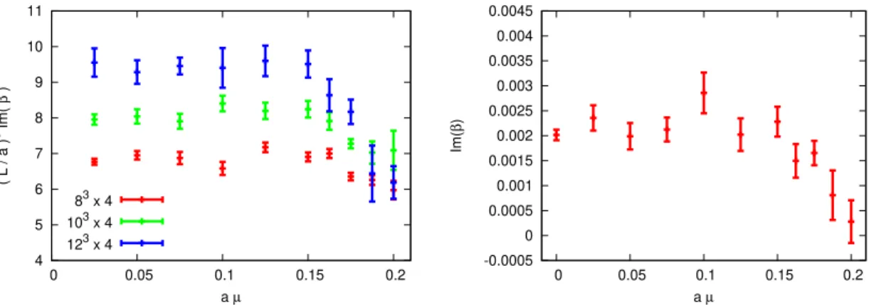
were measured in shorter runs and βc0 was modified by ∆β=β1−βc0 if necessary. Then all further production runs were performed at these βc =βc0+ ∆β. The resulting values are shown in table1. From [59] we also glean that the spatial volume dependence of βc is rather mild and in this first exploratory work we set the same bare coupling for all of our 3 spatial volumes.
JHEP05(2020)088
3.1 Monte-Carlo with µ >0
We would like to generate configurations with the weight |Re detD(U, µ)|e−Sg(U). This is a non-trivial problem and to our knowledge no pseudo-fermion type construction can be found. What one may still do is rewrite the weight as
|Re detD(U, µ)|e−Sg(U)= |Re detD(U, µ)|
|Re detD(U,0)|detD(U,0)e−Sg(U), (3.1) since detD(U,0) is real and positive, and utilize a standard (R)HMC algorithm at µ= 0 and include the µ-dependent ratio in the Metropolis accept/reject step at the end of the trajectory. This will clearly be an expensive algorithm because the full determinant needs to be computed, but with the help of the reduced matrix construction the cost is still manageable for the lattice volumes we will consider in this paper.
Since we are working with rooted staggered fermions we need to compute the full determinant, its square root, its real part and then its sign and absolute value. At finite temperature these steps can most easily be done with the help of the reduced matrix [38].
This has 6(L/a)3 eigenvalues,λi(U), and the main utility of them is that the full staggered determinant can be given at finite chemical potential as,
detDst(U, µ) =Y
i
λi(U)e−2Tµ −e2Tµ
. (3.2)
For the precise definition of the reduced matrix see [38]. We will define the square root branch factor-by-factor in the above product by requiring continuity inµor in other words by requiring that in the µ→0 limit each factor below goes to unity,
detD(U, µ) detD(U,0) =
detDst(U, µ) detDst(U, µ)
1/2
=Y
i
λi(U)e−2Tµ −e2Tµ λi(U)−1
!1/2
. (3.3)
The branch cut of the square root is placed on the negative real axis. This procedure fully fixes the complex determinant ratio. The real part, sign and absolute value can then be taken straightforwardly. Notice that with this procedure the partition function remains real since detD(U∗, µ) = detD(U, µ)∗ for real µ, and so our approach maintains its validity.
Clearly, if µ is small the ratio |Re detD(U, µ)|/|Re detD(U,0)| is close to unity and hence will not affect the Metropolis step much, i.e., a tuned (R)HMC algorithm at µ= 0 will perform just as well. On a given spatial volume as µincreases the ratio will influence the Metropolis step more and more and will decrease the acceptance rate. This can be compensated by employing shorter (R)HMC trajectories as this will change the links less and consequently the change in the ratio with respect to the beginning and end of the trajectory will decrease. In this way we are able to keep the acceptance rate above 50%
for all runs. The shorter trajectories will of course lead to larger autocorrelation times.
Concretely, our estimate of integrated autocorrelation times of our key observable (3.5) are between 50 and 500 depending on µ and L/a. The total number of configurations are between 5·104 and 2·105, leading to a few hundred independent configurations for each simulation point. We observe that “tunnelling” between the +1 and −1 sectors are
JHEP05(2020)088
0 0.2 0.4 0.6 0.8 1
0 0.05 0.1 0.15 0.2
< ε >abs, µ
a µ 83 x 4
103 x 4 123 x 4
0 0.002 0.004 0.006 0.008 0.01 0.012
0 0.01 0.02 0.03 0.04
a2 f ( µ, V )
( a µ )2 83 x 4
103 x 4 123 x 4
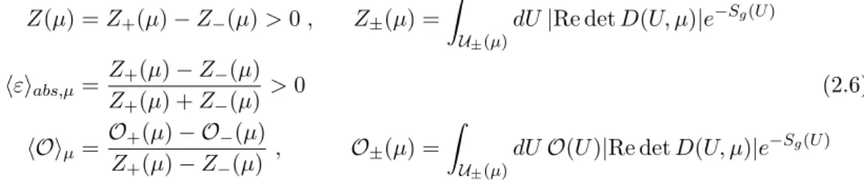
Figure 1. Left: the average sign,hεiabs,µ for the 3 spatial volumes as a function of the chemical potentialµ. Right: the factor f(µ, V) parametrizing the average sign; see (3.4).
frequent, i.e., the change in the µ-dependent ratio is small enough so that even if the trajectory changes sector we observe good acceptance.
The crucial measure of whether the results are reliable or not is given by hεiabs,µ, i.e., the average sign, which at the same time measures the strength of the sign problem itself.
Since hεiabs,µ →1 asµ→0 we parametrize it as,
hεiabs,µ =e−V µ2f(µ,V) (3.4)
with the 4-volumeV =L3/T and show in figure1bothhεiabs,µas well asf(µ, V). Clearly, f(µ, V) depends mildly on V but does depend non-trivially on µ. As can be seen the volumes L/a = 8,10,12 and chemical potentials aµ ≤ 0.2 are safely in the region where hεiabs,µ is several standard deviations away from zero, hence the sign reweighting (2.5) can be performed without issues. In particular, as emphasized, there is no overlap problem to contend with.
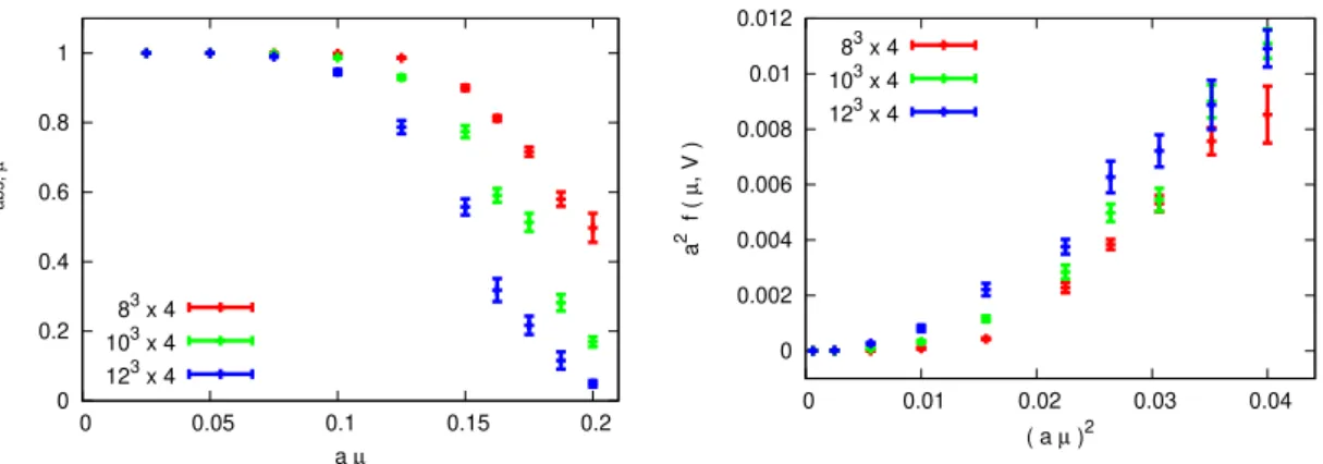
It is worth exploring what the effect of the sign reweighting is on some observables, more precisely how different some observables are in the +1 and−1 sectors. As an example we show the gauge action per unit space time volume in figure2as a function of the chemical potential separately for the two sectors.
3.2 Fisher zeros
Once it has been determined which volumes and chemical potentials allow for the ap- plication of the sign reweighting (2.5) we are able to compute observables. Since our primary interest is the order of the phase transition as a function of µwe will compute the Fisher zeros in the bare coupling β, i.e., we will look for complex bare couplings such that Z(µ, β) = 0 at given µand volume; see (2.6). This amounts to measuring the observables
O(U) =e−(β−βc)
Sg(U)
βc (3.5)
for complexβ, assuming the simulation was done at (real) bare couplingβc. SinceO(U∗) = O(U) our method can be applied without problems. More precisely, since Z(µ, β) has
JHEP05(2020)088
3.02 3.04 3.06 3.08 3.1 3.12 3.14
0 0.05 0.1 0.15 0.2
Sg a4 / V
a µ 83 x 4 +1
-1
3.03 3.04 3.05 3.06 3.07 3.08 3.09 3.1 3.11 3.12 3.13 3.14
0 0.05 0.1 0.15 0.2
a µ 103 x 4 +1
-1
3.02 3.04 3.06 3.08 3.1 3.12 3.14
0 0.05 0.1 0.15 0.2
Sg a4 / V
a µ 123 x 4 +1
-1
Figure 2. The gauge action per unit space time volume Sg a4/V = Sg (a/L)3 aT for the 3 spatial volumes and the sectors +1 and−1 separately. For the low chemical potentials there are no configurations within the sector−1 in our ensembles.
several zeros as a function of complex β, we will be looking for the one closest to the real axis, which in every run happens to coincide with the one closest to (βc,0) in the complex plane as well. This zero will be called the leading zero.
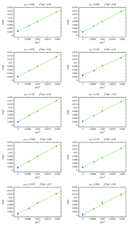
The volume scaling of Imβ determines the order of the transition: if Imβ →const as L/a → ∞ the transition is a cross-over, if Imβ ∼a3/L3 the transition is first order and finally if Imβ ∼(a/L)α with a non-trivial exponent α >0 the transition is second order.
Although these leading order expressions are unambiguous in all three cases, the subleading terms are a priori not known. Since we know that atµ= 0 the transition is a cross-over for physical quark masses, it is generally expected that for small µit will stay a cross-over. At fixed µ > 0 the imaginary part of the leading Fisher zero is then extrapolated to infinite volume via,
Imβ =A+B(a/L)3 , (3.6)
where the exponent 3 in the subleading term is merely an ansatz. In this first study we only simulated at 3 volumes,L/a= 8,10,12 and hence we are unable to fit the exponent of the subleading term simultaneously withA andB. Empirically, we do find that the above fit function provides acceptable statistical fits for our choice of chemical potentials.
JHEP05(2020)088
4 5 6 7 8 9 10 11
0 0.05 0.1 0.15 0.2
( L / a )3 Im( β )
a µ 83 x 4
103 x 4 123 x 4
-0.0005 0 0.0005 0.001 0.0015 0.002 0.0025 0.003 0.0035 0.004 0.0045
0 0.05 0.1 0.15 0.2
Im(β)
a µ
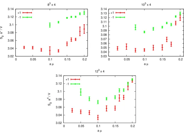
Figure 3. Left: the measured imaginary parts of the Fisher zeros scaled by the spatial volume.
Right: the infinite volume extrapolated imaginary part of the Fisher zeros. The result atµ= 0 was obtained using the standard (R)HMC algorithm.
The existence of a critical end point would suggest that Imβ∞(µ) =A(µ) is a decreas- ing function of µand as µ→µc we have A(µ)→0.
The real part of the leading Fisher zero on the other hand may be used to define the critical coupling. The simulations we performed at particular values of βc =βc(µ) and we have checked that for aµ > 0.1 the differences ∆β = Reβ −βc are deviating from zero less than 3σ and rarely beyond 1.5σ. Note that a smooth cross-over means that different observables may lead to different definitions of the pseudo-critical coupling.
The measured imaginary parts of the Fisher zeros are shown in the left panel of figure3.
The extrapolations to infinite volume using L/a= 8,10,12 are shown in figure 4 together with the resultingχ2/dof values of the fits. Out of the 10 extrapolations the largestχ2/dof values are at aµ = 0.1, 0.1875, 0.2 and are 4.3, 2.37, 2.95. Note that dof = 1 and even the largest χ2/dof = 4.3 leads to a q-value of 4%. The resulting Im (β∞(µ)) as a function of µis finally shown in the right panel of figure3.
The most important result from our investigation can be gleaned from figure 3. Both at finite volumes and correspondingly in infinite volume the imaginary part of the rele- vant Fisher zero is decreasing as the chemical potential becomes sufficiently large. More precisely, the infinite volume extrapolated result shows that the imaginary part of the lead- ing Fisher zero is more or less flat up to aµ ∼ 0.15 and a sharp decrease is observed for 0.15 ≤aµ ≤0.2. The observed flatness agrees within errors with the slight increase seen in [42, 59], and cannot be significantly distinguished from it with the currently available statistics. This means that in the range of chemical potentials where our results are re- liable with trustworthy statistical errors, i.e., hεiabs,µ 6= 0, we are able to conclude with high statistical significance that the leading singularity of logZ is eventually moving closer and closer to the real axis. In fact, the location of the singularity is consistent with a real value at aµ ∼ 0.2. This in turn means that the strength of the transition is eventually increasing and very suggestive that a true phase transition occurs at around aµ ∼ 0.2.
This corresponds toµ/Tc ∼0.8, in agreement with [42], however the latter result should be interpreted with caution since, as we explained, we do not expect the fixed Nt= 4 results
JHEP05(2020)088
0 0.002 0.004 0.006 0.008 0.01 0.012 0.014 0.016
0 0.0005 0.001 0.0015 0.002
Im(β)
(a/L)3 a µ = 0.025 χ2/dof = 0.09
0 0.002 0.004 0.006 0.008 0.01 0.012 0.014 0.016
0 0.0005 0.001 0.0015 0.002
Im(β)
(a/L)3 a µ = 0.050 χ2/dof = 0.38
0 0.002 0.004 0.006 0.008 0.01 0.012 0.014 0.016
0 0.0005 0.001 0.0015 0.002
Im(β)
(a/L)3 a µ = 0.075 χ2/dof = 0.00
0 0.002 0.004 0.006 0.008 0.01 0.012 0.014 0.016
0 0.0005 0.001 0.0015 0.002
Im(β)
(a/L)3 a µ = 0.100 χ2/dof = 4.30
0 0.002 0.004 0.006 0.008 0.01 0.012 0.014 0.016
0 0.0005 0.001 0.0015 0.002
Im(β)
(a/L)3 a µ = 0.125 χ2/dof = 0.03
0 0.002 0.004 0.006 0.008 0.01 0.012 0.014 0.016
0 0.0005 0.001 0.0015 0.002
Im(β)
(a/L)3 a µ = 0.150 χ2/dof = 1.02
0 0.002 0.004 0.006 0.008 0.01 0.012 0.014 0.016
0 0.0005 0.001 0.0015 0.002
Im(β)
(a/L)3 a µ = 0.1625 χ2/dof = 0.66
0 0.002 0.004 0.006 0.008 0.01 0.012 0.014 0.016
0 0.0005 0.001 0.0015 0.002
Im(β)
(a/L)3 a µ = 0.175 χ2/dof = 0.94
0 0.002 0.004 0.006 0.008 0.01 0.012 0.014 0.016
0 0.0005 0.001 0.0015 0.002
Im(β)
(a/L)3 a µ = 0.1875 χ2/dof = 2.37
0 0.002 0.004 0.006 0.008 0.01 0.012 0.014 0.016
0 0.0005 0.001 0.0015 0.002
Im(β)
(a/L)3 a µ = 0.200 χ2/dof = 2.95
Figure 4. The infinite volume extrapolations (3.6) of the imaginary parts of the leading Fisher zeros at the various chemical potentials we have simulated at.
JHEP05(2020)088
to be particularly close to the continuum with our chosen discretization. Nonetheless our results are trustworthy in the well defined statistical model given by the Nt = 4 lattice system.
4 Conclusion and outlook
In this paper we have introduced a new technique for evaluating the path integral at finite baryon chemical potential. The approach involves generating configurations by the absolute value of the real part of the fermionic determinant and taking the signs into account by a discrete reweighting. The first step necessitates the evaluation of the full determinant during the Monte-Carlo simulation which makes the algorithm rather costly but still manageable for 83×4, 103×4 and 123×4 which are the volumes we used. The second step, the discrete reweighting by the sign of the real part of the fermionic determinant, is a fully controlled step provided the average sign is several standard deviations away from zero, i.e., the sign problem is not too severe. This requirement can be easily monitored and once it is fulfilled, the results are completely trustworthy with well-defined statistical errors.
This feature is the main advantage of our method. It improves on traditional reweighting in µ and/or some other continuous parameter because in that case the notorious overlap problem may invalidate the results even though a naive application of the reweighting formulahOiµ=hOwi0/hwi0 seemingly presents no problems.
Since our main interest was the order of the thermal phase transition as a function of the chemical potential, we have determined the first few Fisher zeros and the volume scaling of the leading one (the one closest to the real axis) for 10 choices of µin the range 0.025≤ aµ ≤ 0.2. We have observed that the strength of the phase transition stays flat within errors for 0< aµ <0.15 and increases sharply for 0.15< aµ <0.2, signified by the decrease in the imaginary part of the leading Fisher zero. The infinite volume extrapolation of the leading Fisher zero at aµ∼0.2, corresponding toµB/T ∼2.4, is in fact consistent with a true phase transition, i.e., the imaginary part is consistent with zero.
There are however several avenues to improve on our work in the future. First, we have performed simulations at fixed Nt= 4, i.e., we have not addressed the continuum limit at all; simulations with larger temporal extents would be necessary in order to do so. Once the continuum behavior is investigated it might be worthwhile to use an improved action, both for the gauge and fermionic actions. In the present work we have used the Wilson plaquette gauge action and unimproved staggered fermions. The motivation was to replicate the setup of [42] where the critical end point was investigated using traditional reweighting inµ. It is worth noting that even though the unimproved staggered discretization on Nt= 4 lattices is far from the continuum, it is a well-defined lattice statistical physics model with a sign problem. Hence it makes perfect sense to study it in order to gain valuable insight into the sign problem in general.
Second, the volume scaling of the Fisher zeros is of central importance and our ansatz (3.6) was simply motivated by empirically observing good statistical fits as well as the fact that we only had data on 3 volumes. Hence we were unable to fit all 3 param-
JHEP05(2020)088
eters, A, B and C in the general form,
Imβ =A+B(a/L)C , (4.1)
which would otherwise be the justified procedure. Once an additional volume 143×4 is added, the exponentC could be determined or at least constrained.
Third, we have set the quark masses to their physical values at β =βc atµ= 0 and have not changed them forµ >0 along the line of constant physics. Even though the effect is expected to be negligible relative to other sources of errors, in future work we do plan to follow the line of constant physics for µ >0.
Fourth, we have included the chemical potential at the quark level as µu = µd = µB/3 = µ and µs = 0 which corresponds to µS = µB/3. Nonetheless our method can be trivially modified to include other chemical potential assignments, e.g., strangeness neutrality hSi= 0 or µS= 0.
Finally we mention that the recently introduced geometric matching procedure [43]
provides a new rooting procedure at finite Ntwhich is nonetheless expected to agree with the one followed in this paper towards the continuum limit. We repeated the determination of the leading Fisher zeros using geometric matching and found that they agree with the ones presented in this paper within statistical uncertainties. This type of cross-check will be especially useful for future studies targeting the continuum limit.
Acknowledgments
This work was partially supported by the Hungarian National Research, Development and Innovation Office – NKFIH grant KKP-126769. AP is supported by the J´anos Bolyai Research Scholarship of the Hungarian Academy of Sciences and by the ´UNKP-19-4 New National Excellence Program of the Ministry for Innovation and Technology.
Open Access. This article is distributed under the terms of the Creative Commons Attribution License (CC-BY 4.0), which permits any use, distribution and reproduction in any medium, provided the original author(s) and source are credited.
References
[1] C.R. Allton et al.,The QCD thermal phase transition in the presence of a small chemical potential, Phys. Rev.D 66(2002) 074507[hep-lat/0204010] [INSPIRE].
[2] R.V. Gavai and S. Gupta,Pressure and nonlinear susceptibilities in QCD at finite chemical potentials,Phys. Rev.D 68(2003) 034506 [hep-lat/0303013] [INSPIRE].
[3] R.V. Gavai and S. Gupta,The Critical end point of QCD, Phys. Rev.D 71(2005) 114014 [hep-lat/0412035] [INSPIRE].
[4] C.R. Allton et al.,Thermodynamics of two flavor QCD to sixth order in quark chemical potential, Phys. Rev.D 71(2005) 054508[hep-lat/0501030] [INSPIRE].
[5] R.V. Gavai and S. Gupta,QCD at finite chemical potential with six time slices,Phys. Rev.D 78(2008) 114503[arXiv:0806.2233] [INSPIRE].
JHEP05(2020)088
[6] MILCcollaboration, QCD equation of state at non-zero chemical potential, PoS(LATTICE2008)171(2008) [arXiv:0910.0276] [INSPIRE].
[7] S. Bors´anyi, Z. Fodor, S.D. Katz, S. Krieg, C. Ratti and K. Szabo, Fluctuations of conserved charges at finite temperature from lattice QCD,JHEP 01(2012) 138[arXiv:1112.4416]
[INSPIRE].
[8] S. Bors´anyi et al.,QCD equation of state at nonzero chemical potential: continuum results with physical quark masses at ordermu2,JHEP 08(2012) 053[arXiv:1204.6710] [INSPIRE].
[9] R. Bellwied et al.,Fluctuations and correlations in high temperature QCD,Phys. Rev. D 92 (2015) 114505[arXiv:1507.04627] [INSPIRE].
[10] H.T. Ding, S. Mukherjee, H. Ohno, P. Petreczky and H.P. Schadler,Diagonal and off-diagonal quark number susceptibilities at high temperatures,Phys. Rev. D 92(2015) 074043[arXiv:1507.06637] [INSPIRE].
[11] A. Bazavov et al.,The QCD Equation of State to O(µ6B)from Lattice QCD,Phys. Rev.D 95(2017) 054504[arXiv:1701.04325] [INSPIRE].
[12] HotQCDcollaboration,Chiral crossover in QCD at zero and non-zero chemical potentials, Phys. Lett.B 795(2019) 15 [arXiv:1812.08235] [INSPIRE].
[13] M. Giordano and A. P´asztor,Reliable estimation of the radius of convergence in finite density QCD,Phys. Rev. D 99(2019) 114510[arXiv:1904.01974] [INSPIRE].
[14] A. Bazavov et al.,Skewness, kurtosis and the fifth and sixth order cumulants of net
baryon-number distributions from lattice QCD confront high-statistics STAR data,Phys. Rev.
D 101(2020) 074502 [arXiv:2001.08530] [INSPIRE].
[15] P. de Forcrand and O. Philipsen,The QCD phase diagram for small densities from
imaginary chemical potential,Nucl. Phys. B 642(2002) 290[hep-lat/0205016] [INSPIRE].
[16] M. D’Elia and M.-P. Lombardo,Finite density QCD via imaginary chemical potential,Phys.
Rev.D 67(2003) 014505[hep-lat/0209146] [INSPIRE].
[17] M. D’Elia and F. Sanfilippo,Thermodynamics of two flavor QCD from imaginary chemical potentials,Phys. Rev.D 80(2009) 014502 [arXiv:0904.1400] [INSPIRE].
[18] P. Cea, L. Cosmai and A. Papa,Critical line of 2 + 1flavor QCD,Phys. Rev. D 89(2014) 074512[arXiv:1403.0821] [INSPIRE].
[19] C. Bonati, P. de Forcrand, M. D’Elia, O. Philipsen and F. Sanfilippo, Chiral phase transition in two-flavor QCD from an imaginary chemical potential,Phys. Rev.D 90(2014) 074030 [arXiv:1408.5086] [INSPIRE].
[20] P. Cea, L. Cosmai and A. Papa,Critical line of 2 + 1flavor QCD: Toward the continuum limit,Phys. Rev.D 93 (2016) 014507[arXiv:1508.07599] [INSPIRE].
[21] C. Bonati, M. D’Elia, M. Mariti, M. Mesiti, F. Negro and F. Sanfilippo, Curvature of the chiral pseudocritical line in QCD: Continuum extrapolated results,Phys. Rev. D 92(2015) 054503[arXiv:1507.03571] [INSPIRE].
[22] R. Bellwied et al., The QCD phase diagram from analytic continuation,Phys. Lett.B 751 (2015) 559[arXiv:1507.07510] [INSPIRE].
[23] M. D’Elia, G. Gagliardi and F. Sanfilippo, Higher order quark number fluctuations via imaginary chemical potentials inNf = 2 + 1QCD,Phys. Rev.D 95 (2017) 094503 [arXiv:1611.08285] [INSPIRE].
JHEP05(2020)088
[24] J.N. Guenther et al.,The QCD equation of state at finite density from analytical continuation,Nucl. Phys. A 967(2017) 720[arXiv:1607.02493] [INSPIRE].
[25] P. Alba et al.,Constraining the hadronic spectrum through QCD thermodynamics on the lattice,Phys. Rev.D 96(2017) 034517 [arXiv:1702.01113] [INSPIRE].
[26] V. Vovchenko, A. Pasztor, Z. Fodor, S.D. Katz and H. Stoecker, Repulsive baryonic
interactions and lattice QCD observables at imaginary chemical potential,Phys. Lett.B 775 (2017) 71[arXiv:1708.02852] [INSPIRE].
[27] C. Bonati, M. D’Elia, F. Negro, F. Sanfilippo and K. Zambello,Curvature of the
pseudocritical line in QCD: Taylor expansion matches analytic continuation,Phys. Rev.D 98(2018) 054510[arXiv:1805.02960] [INSPIRE].
[28] S. Bors´anyi et al.,Higher order fluctuations and correlations of conserved charges from lattice QCD, JHEP 10(2018) 205[arXiv:1805.04445] [INSPIRE].
[29] R. Bellwied et al.,Off-diagonal correlators of conserved charges from lattice QCD and how to relate them to experiment,Phys. Rev.D 101(2020) 034506[arXiv:1910.14592] [INSPIRE].
[30] S. Bors´anyi et al.,The QCD crossover at finite chemical potential from lattice simulations, arXiv:2002.02821[INSPIRE].
[31] E. Seiler, D. Sexty and I.-O. Stamatescu, Gauge cooling in complex Langevin for QCD with heavy quarks,Phys. Lett. B 723(2013) 213[arXiv:1211.3709] [INSPIRE].
[32] D. Sexty,Simulating full QCD at nonzero density using the complex Langevin equation, Phys. Lett.B 729(2014) 108[arXiv:1307.7748] [INSPIRE].
[33] G. Aarts, E. Seiler, D. Sexty and I.-O. Stamatescu, Simulating QCD at nonzero baryon density to all orders in the hopping parameter expansion,Phys. Rev. D 90(2014) 114505 [arXiv:1408.3770] [INSPIRE].
[34] Z. Fodor, S.D. Katz, D. Sexty and C. T¨or¨ok, Complex Langevin dynamics for dynamical QCD at nonzero chemical potential: A comparison with multiparameter reweighting, Phys.
Rev.D 92(2015) 094516[arXiv:1508.05260] [INSPIRE].
[35] D. Sexty,Calculating the equation of state of dense quark-gluon plasma using the complex Langevin equation, Phys. Rev.D 100(2019) 074503[arXiv:1907.08712] [INSPIRE].
[36] J.B. Kogut and D.K. Sinclair,Applying Complex Langevin Simulations to Lattice QCD at Finite Density,Phys. Rev.D 100(2019) 054512[arXiv:1903.02622] [INSPIRE].
[37] M. Scherzer, D. Sexty and I.O. Stamatescu,Deconfinement transition line with the Complex Langevin equation up toµ/T ∼5,arXiv:2004.05372[INSPIRE].
[38] A. Hasenfratz and D. Toussaint,Canonical ensembles and nonzero density quantum chromodynamics,Nucl. Phys. B 371(1992) 539[INSPIRE].
[39] I.M. Barbour, S.E. Morrison, E.G. Klepfish, J.B. Kogut and M.-P. Lombardo, Results on finite density QCD,Nucl. Phys. Proc. Suppl.60A(1998) 220[hep-lat/9705042] [INSPIRE].
[40] Z. Fodor and S.D. Katz, A New method to study lattice QCD at finite temperature and chemical potential,Phys. Lett.B 534(2002) 87 [hep-lat/0104001] [INSPIRE].
[41] Z. Fodor and S.D. Katz, Lattice determination of the critical point of QCD at finite T and mu,JHEP 03(2002) 014[hep-lat/0106002] [INSPIRE].
[42] Z. Fodor and S.D. Katz, Critical point of QCD at finite T and mu, lattice results for physical quark masses,JHEP 04(2004) 050[hep-lat/0402006] [INSPIRE].
JHEP05(2020)088
[43] M. Giordano, K. Kapas, S.D. Katz, D. Nogradi and A. Pasztor, Radius of convergence in lattice QCD at finiteµB with rooted staggered fermions,Phys. Rev. D 101(2020) 074511 [arXiv:1911.00043] [INSPIRE].
[44] AuroraSciencecollaboration,New approach to the sign problem in quantum field theories:
High density QCD on a Lefschetz thimble, Phys. Rev.D 86(2012) 074506 [arXiv:1205.3996] [INSPIRE].
[45] M. Cristoforetti, F. Di Renzo, A. Mukherjee and L. Scorzato, Monte Carlo simulations on the Lefschetz thimble: Taming the sign problem,Phys. Rev. D 88(2013) 051501
[arXiv:1303.7204] [INSPIRE].
[46] A. Alexandru, G. Basar and P. Bedaque,Monte Carlo algorithm for simulating fermions on Lefschetz thimbles,Phys. Rev.D 93(2016) 014504 [arXiv:1510.03258] [INSPIRE].
[47] A. Alexandru, G. Basar, P.F. Bedaque, G.W. Ridgway and N.C. Warrington,Fast estimator of Jacobians in the Monte Carlo integration on Lefschetz thimbles,Phys. Rev. D 93(2016) 094514[arXiv:1604.00956] [INSPIRE].
[48] J. Nishimura and S. Shimasaki, Combining the complex Langevin method and the generalized Lefschetz-thimble method,JHEP 06(2017) 023[arXiv:1703.09409] [INSPIRE].
[49] C. Gattringer, New developments for dual methods in lattice field theory at non-zero density, PoS(LATTICE2013)002(2014) [arXiv:1401.7788] [INSPIRE].
[50] C. Marchis and C. Gattringer,Dual representation of lattice QCD with worldlines and worldsheets of abelian color fluxes,Phys. Rev.D 97(2018) 034508 [arXiv:1712.07546]
[INSPIRE].
[51] G. Aarts, E. Seiler and I.-O. Stamatescu,The Complex Langevin method: When can it be trusted?, Phys. Rev.D 81(2010) 054508[arXiv:0912.3360] [INSPIRE].
[52] G. Aarts, F.A. James, E. Seiler and I.-O. Stamatescu, Complex Langevin: Etiology and Diagnostics of its Main Problem,Eur. Phys. J.C 71(2011) 1756 [arXiv:1101.3270]
[INSPIRE].
[53] P. de Forcrand, S. Kim and T. Takaishi,QCD simulations at small chemical potential,Nucl.
Phys. Proc. Suppl.119(2003) 541[hep-lat/0209126] [INSPIRE].
[54] P. de Forcrand,Simulating QCD at finite density,PoS(LAT2009)010(2009) [arXiv:1005.0539] [INSPIRE].
[55] S.D.H. Hsu and D. Reeb, On the sign problem in dense QCD,Int. J. Mod. Phys. A 25 (2010) 53[INSPIRE].
[56] A. Alexandru, M. Faber, I. Horvath and K.-F. Liu, Lattice QCD at finite density via a new canonical approach,Phys. Rev.D 72 (2005) 114513[hep-lat/0507020] [INSPIRE].
[57] A. Li, A. Alexandru, K.-F. Liu and X. Meng,Finite density phase transition of QCD with Nf = 4andNf = 2 using canonical ensemble method,Phys. Rev. D 82(2010) 054502 [arXiv:1005.4158] [INSPIRE].
[58] A. Li, A. Alexandru and K.-F. Liu, Critical point ofNf = 3 QCD from lattice simulations in the canonical ensemble,Phys. Rev. D 84(2011) 071503[arXiv:1103.3045] [INSPIRE].
[59] M. Giordano, K. Kapas, S.D. Katz, D. Nogradi and A. Pasztor, The effect of stout smearing on the phase diagram from multiparameter reweigthing in lattice QCD,arXiv:2003.04355 [INSPIRE].