Simulation and numerical methods Energy modeling
for buildings and components
2
Simulation and numerical methods Energy modeling
for buildings and components
Michele De Carli
TERC Kft. • Budapest, 2013
© Michele De Carli, 2013
3
End of manuscript / Kézirat lezárva: 2012. december 31.
ISBN 978-963-9968-81-3
Published by TERC Ltd / Kiadja a TERC Kereskedelmi és Szolgáltató Kft. Szakkönyvkiadó Üzletága, az 1795-ben alapított Magyar Könyvkiadók és Könyvterjesztők Egyesülésének
a tagja
A kiadásért felel: a kft. ügyvezető igazgatója Felelős szerkesztő: Lévai-Kanyó Judit
Műszaki szerkesztő: TERC Kft.
Terjedelem: 7,25 szerzői ív
4
CONTENT
1. INTRODUCTION ...17
2. INDOOR AND WEATHER CONDITIONS ...20
2.1 Thermal comfort ...20
2.1.1 Global thermal comfort conditions ...20
2.1.2 Local discomfort conditions ...21
2.1.3 Adaptive comfort conditions for unconditioned buildings ...22
2.2 Indoor Air Quality and ventilation requirements ...24
2.3 Climatic conditions ...26
2.3.1 Outdoor temperature ...26
2.3.2 Solar radiation ...32
2.3.3 Relative humidity and water vapour ...45
2.3.4 Wind ...47
3. HEAT CONDUCTION IN BUILDING ELEMENTS ...48
3.1 The problem of thermal conduction ...48
3.2 Thermal conduction in steady state conditions in a linear element ...50
3.2.1 Thermal transmittance of a building component ...51
3.2.2 Thermal bridges ...51
3.2.3 Building elements containing pipes ...54
3.3 Thermal conduction in dynamic conditions ...55
3.3.1 Electrical analogy ...55
3.3.2 Numerical solutions ...58
3.2.3 Building elements containing pipes ...63
4. MODELS FOR THE THERMAL BALANCE OF A ROOM ...69
4.1 Steady state model ...69
4.2 External resistance with internal capacitance ...71
4.3 Quasi steady state model ...76
4.3.1 Building energy demand for space heating ...76
4.3.2 Building energy demand for space cooling ...77
4.3 Detailed model of the thermal balance of a room ...78
4.3.1 Equations for the thermal balance ...78
4.3.2 Convective heat exchange ...82
4.3.3 Radiant heat exchange ...84
4.3.4 Solar energy through windows ...85
4.3.5 Solar radiation modelling in the rooms ...95
4.3.6 Example of a balance in steady state conditions ...99
4.4 Detailed models for rooms equipped with radiant systems ... 101
4.5 Boundary conditions on external surfaces ... 104
4.5.1 Sol-air temperature ... 104
4.5.2 Heat exchange with the sky ... 105
5
4.6 Models based on the thermal response of the room ... 106
4.6.1 Method based on equivalent difference temperature ... 106
4.6.2 Method for the transfer functions of the room ... 108
4.6.3 Method of the periodic transfer functions ... 111
6
LIST OF NOTATIONS
a thermal diffusivity [m2/s]
A extraterrestrial solar radiation if the rays were at the zenith [W/m2]
Ab coefficient for the solar radiation passing through the reference glazing element [-]
Ad coefficient for the solar radiation passing through the reference glazing element [-]
AM Air Mass [-]
B atmospheric extinction [-]
B’ shape factor of basement for losses through the ground [m]
Bb coefficient for the solar radiation passing through the reference glazing element [-]
Bd coefficient for the solar radiation passing through the reference glazing element [-]
bj conduction transfer function coefficient [W/(m2 K)]
bu coupling factor [-]
bz transfer functions [-]
c specific heat of the medium [kJ/(kg K)] or [J/(kg K)]
C diffuse solar radiation coefficient [-]
C heat capacity [J/K]
cj conduction transfer function coefficient [W/(m2 K)]
CL cooling load [W]
CLc cooling load from strictly convective heat gain elements [W]
cpa specific heat at constant pressure of the air [kJ/(kg K)] or [J/(kg K)]
cpv specific heat at constant pressure of the vapour [kJ/(kg K)] or [J/(kg K)]
cR common ratio [-]
Cs shading coefficient [-]
cva specific heat capacity of air at constant volume [kJ/(kg K)] or [J/(kg K)]
cw specific heat of the water [kJ/(kg K)] or [J/(kg K)]
D transfer functions [-]
d generic day [-]
DD degree day [°C day]
De equivalent diameter [m]
dj conduction transfer function coefficient [-]
dp outer diameter of the pipe [m]
dQe heat exchange by the generic thermodynamic system [J]
dQi heat generation inside the generic thermodynamic system [J]
DR Draft Risk [-]
dU variation of internal energy of the generic thermodynamic system [J]
d1 the first day of the considered month [-]
d2 the last day of the considered month [-]
E efficiency of the heat recovery system [-]
E(λ) energy intensity of the solar radiation [W/m3] ER extraction rate [W]
ERmax ER value when ta is above the throttling range [W]
ERmin ER value when ta is below the throttling range [W]
fa attenuation factor of the room for the solar radiation [-]
7
fc coefficient which takes into account the effect of changes in the radiant heat exchange variations with respect to the overall internal heat exchange coefficient [-]
Fc fraction of the input energy which can be lost back to the surroundings [W/m]
fg1 coefficient which considers the annual variation of outdoor temperature [-]
fg2 coefficient which takes into account the change in outdoor temperature [-]
fij coupling factor between rooms i and j at different temperature [-]
Fo Fourier number [-]
Fi-j view factor between the i-th and the j-th surfaces [-]
Fp-k view factor between the human body and the k-th surface [-]
fRsi temperature factor, the minimum internal surface temperature [-]
fs internal gain storage factor of the room [-]
Fs factor of the secondary specific effective mass of the room [-]
fsh shading factor [-]
g gravity acceleration [m/s2] g g-factor for a glazing system [-]
Ga,z air flow rate [kg/s]
gr coefficients depending on the thermal inertia of the constructions [W/K]
Gv,in internal vapour production [kg/s]
Gv,p vapour generation/extraction due to the plant [kg/s]
Gw factor considering the aquifer below the ground [-]
h barometric height [m]
h specific enthalpy of the mixture air-vapour [kJ/kg]
H heat loss coefficient [W/K]
ha specific enthalpy of the air [kJ/kg]
hc convective heat exchange coefficient [W/(m2 K)]
HG heat gain [W]
Hm monthly average solar radiation on the horizontal [kWh/(m2 month)] or [kJ/(m2 month)]
0 ,
Hm monthly average solar radiation on the horizontal [kWh/(m2 month)] or [kJ/(m2 month)]
hr radiant heat exchange coefficient [W/(m2 K)]
hs overall surface heat exchange coefficient [W/(m2 K)]
hse overall external surface heat exchange coefficient [W/(m2 K)]
hsi overall internal surface heat exchange coefficient [W/(m2 K)]
hv specific enthalpy of the vapour [kJ/kg]
Hy yearly incident solar energy over a differently oriented and inclined plane [kWh/(m2 year)] or [kJ/(m2 year)]
0 ,
Hy yearly incident solar energy on the horizontal plane [kWh/(m2 year)] or [kJ/(m2 year)]
I incident solar radiation [W/m2] I intensity current [A]
I* corrected solar radiation [W/m2] Ia absorbed solar radiation [W/m2] Ib direct radiation [W/m2]
IbN direct normal solar radiation [W/m2]
Id diffuse solar radiation which reaches the generic surface [W/m2]
IdH diffuse solar radiation striking the ground on an horizontal plane [W/m2]
8 Id,0 diffuse radiation on horizontal [W/m2]
Ig solar radiation reflected by the ground [W/m2] Igl solar radiation transmitted through the glass [W/m2]
I&i incoming intensity current [A]
I&o outgoing intensity current [A]
Ir reflected solar radiation [W/m2]
Iref,gl solar radiation entering the room through a reference glazing surface [W/m2] Isc solar constant [W/m2]
It transmitted solar radiation [W/m2] IT overall solar radiation [W/m2]
IT,0 overall solar radiation on horizontal [W/m2]
Ix maximum solar radiation on the considered orientation passing through the reference glass [W/m2]
I1(i) radiation leaving the i-th glass on the external surface [W/m2] I2(i) radiation leaving the i-th glass on the internal surface [W/m2] k thermal conductivity of the medium [W/(m K)]
K unit length conductance between the space air and surroundings [W/(m K)]
k* equivalent thermal conductivity of the medium [W/(m K)]
Kcluod cloudiness factor [-]
Kh cloudiness index [-]
kp thermal conductivity of the pipe [W/(m K)]
ks thermal conductivity of the material embedding the pipes[W/(m K)]
l length [m]
LF length of the space exterior wall [m]
L2D overall specific heat flow exiting the thermal bridge [W/K]
M metabolic rate [W]
ma mass of the air [kg]
Ma the whole air mass of the room [kg]
m&a air mass flow rate [kg/s]
mf specific mass of the wall per surface area [kg/m2] Mp average primary specific effective mass [kg/m2] MR thermal capacity of the room [kg/m2]
m &
sp specific mass flow rate per unit area [kg/(m2 s)]mv mass of the vapour [kg]
n number of sunny hours [-]
n r
normal direction to the generic surface [-]
N average maximum theoretical number of hours of the day [-]
nd,z number of days of the z-th month [-]
Ni shape functions [-]
O(τ) response factor of the system [-]
pa pressure of the air [Pa]
P pipe spacing [m]
P perimeter of the external walls [m]
patm atmospheric pressure [Pa]
p0 atmospheric pressure at sea level [Pa]
ph coefficient for determining the hourly value of outdoor air in cooling conditions [-]
PMV Predicted Mean Vote [-]
9 PPD Percentage People Dissatisfied [%]
pr coefficients depending on the thermal inertia of the constructions [-]
psat saturated vapour pressure of water at those conditions [Pa]
psat,cr saturation pressure corresponding to the critical relative humidity RHcr [Pa]
ptot total pressure of the air-water mixture [Pa]
pv partial pressure of water vapour in the air-water mixture [Pa]
q* specific heat flux (per unit area) across a surface [W/m2] qc convective heat flow [W]
QC,gn total heat gains (solar radiation and internal loads) for the cooling mode [kWh]
QC,ht total heat transfer for the cooling mode [kWh]
Q-C,ht part of the total heat transfer which becomes extra load to be removed [kWh]
QC,ht,extra surplus of heat loss which cannot be used [kWh]
QC,nd building energy need for space cooling in the reference period for a room [kWh]
qC,int convective internal gains [W]
qd conduction heat flow [W]
qd,opaque incoming heat flow due to conduction through opaque walls [W]
qd,window incoming heat flow due to conduction through windows [W]
qg convective heat flow due to the incoming and outgoing air rates in the room [W]
QH,gn total heat loads (solar radiation and internal loads) for the heating mode [kWh]
QH,gn,extra heat loads which cannot be used in the heating mode [kWh]
QH,ht total heat transfer for the heating mode [kWh]
QH,nd building energy need for space heating in the reference period [kWh]
q&i incoming heat flow [W]
ql radiant heat flow due to lighting or other internal gains [W]
q&o outgoing heat flow [W]
qp convective heat power of the internal plants [W]
qr,i infrared radiation heat flow of i-th surface with other surfaces [W]
qs high frequency radiant heat flow due to solar radiation [W]
qT transmission losses [W]
qV ventilation losses [W]
r specific resistance [Ω/m]
r distance between the centres of surfaces [m]
R thermal resistance [m2 K/W]
Rceil thermal resistance of the ceiling [m2 K/W]
Rcl clothing resistance [m2 K/W]
Rfloor thermal resistance of the floor [m2 K/W]
RH relative humidity [-]
RHcr critical surface condensation corresponding to moisture problems [-]
Rp pipe wall resistance [m2 K/W]
Rs surface thermal resistance [m2 K/W]
Rsi internal surface thermal resistance [m2 K/W]
Rse external surface thermal resistance [m2 K/W]
RTF room transfer function
Rtot overall thermal resistance [m2 K/W]
Rw thermal resistance between the mean temperature of the water and the temperature of the inner surface of the pipe [m2 K/W]
Rwindow overall resistance of the window [m2 K/W]
10
Rz resistance connecting the water supply temperature and the logarithmic mean temperature of the water along the circuit [m2 K/W]
Rx thermal resistance between the external surface of the pipe and the pipe level [m2 K/W]
r0 specific latent heat of the water [kJ/kg]
Sk area of the k-th surface [m2]
S parameter characterizing performance of specific types of cooling equipment [W/K]
SATF Space Air Transfer Function Sg area of the floor [m2]
sp thickness of the pipe [m]
sq thickness of each layer composing the wall [m]
s1 thicknesses of the of the sub-slab upper layer [m]
s2 thicknesses of the of the sub-slab lower layer [m]
t temperature [°C]
t’ temperature at the time step τ+∆τ [°C]
ta dry-bulb temperature of the air [°C]
(ta)-∆τ temperature of air at the previous time step [°C]
ta* set point temperature of the control system [°C]
tac constant room air temperature [°C]
tamb,h outdoor temperature at hour h [°C]
tamb,max maximum outdoor air design temperature in cooling conditions [°C]
j d
tamb, , daily mean outdoor temperature of day j [°C]
z m
tamb, , mean outdoor monthly temperature of the z-th month [°C]
Tamb,sat absolute saturation temperature of the outdoor air [K]
TF Transposition Factor [-]
ti indoor operative temperature [°C]
t&i incoming temperature [°C]
tm,amb yearly average outdoor temperature [°C]
tmr mean radiant temperature [°C]
tmw logarithmic mean temperature of the water along the circuit [°C]
to operative temperature [°C]
t&o outgoing temperature [°C]
tPL average temperature at the pipe level in steady state conditions [°C]
tpr plane radiant temperature [°C]
Ts absolute surface temperature [K]
tsa sol-air temperature [°C]
tse external surface temperature [°C]
tscreen temperature of the screen [°C]
tsi internal surface temperature [°C]
tsi,min minimum internal surface temperature for moisture problems [°C]
Tsky absolute fictive sky temperature [K]
Ts,m mean value of absolute surface temperature [K]
tu temperature of the unconditioned space [°C]
Tu the local turbulence intensity [-]
twater,In water supply temperature [°C]
u specific internal energy of the medium [J/m3] U transmittance of a wall (U-value) [W/(m2 K)]
11
Uequiv,g corrected U-value for losses through the ground [W/(m2 K)]
Um mean thermal transmittance [W/(m2 K)]
uz transfer functions [-]
V voltage [V]
V(λ) sensitivity of the human eye to the visible radiation [-]
va air velocity [m/s]
vp coefficients of the RTF [-]
V&i incoming voltage [V]
V&o outgoing voltage [V]
Vol volume [m3] ol
V& volume flow rate [m3/s]
w angle defining the day
W parameter characterizing performance of specific types of cooling equipment [W]
wp coefficients of the RTF [-]
z z direction in the space [m]
Zb→ d response factor between the b-th surface (impulse) and the d-th surface (response) [W/(m2 K)]
Z'b→ d modified response factor between the b-th surface and the d-th surface [W/(m2 K)]
x x direction in the space [m]
y y direction in the space [m]
Greek symbols:
α attenuation constant [-]
α coefficient of sorption [-]
β phase constant [m]
β solar height [°]
Γ thermal conductance [W/(m2 K)]
γ& propagation constant [s0.5/m]
δ Sun’s declination [°]
∆τ considered time step [s]
∆tamb temperature range of outdoor air in cooling conditions [°C]
∆x element thickness in the x direction in the space [m]
ε emissivity of a surface [-]
εi emissivity of the i-th surface [-]
ε0 emittance of the clear sky [-]
φ latitude of point P [°]
φ angle between the segment connecting the centres and the surface normal n [°]
Φa albedo radiation [W/m2] Φd diffuse radiation [W/m2]
Φint radiation due to internal gains [W/m2] λ wavelength of the solar radiation [nm]
λmax maximum peak of the emitted spectral solar radiation of a black body [µm]
ηC,ht dimensionless utilization factor for heat losses [-]
12
ηH,gn dimensionless gain utilization factor for the heating mode [-]
Η intensity of internal heat generation [W/m3] µ longitude of point P [°]
µ0 longitude of the central meridian of the considered location [°]
µp effective primary mass [kg/m2] µs effective secondary mass [kg/m2]
ψ linear coefficient of the heat loss for a thermal bridge [W/(m K)]
ψe heat loss linear coefficient for a thermal bridge considering external dimensions [W/(m K)]
ψi heat loss linear coefficient for a thermal bridge considering internal net dimensions [W/(m K)]
ψoi heat loss linear coefficient for a thermal bridge considering internal gross dimensions [W/(m K)]
ψsolar solar azimuth [°]
ψsurface surface azimuth [°]
ϑ incident angle of solar radiation, i.e. angle between normal direction of the surface and the solar direct radiation [°]
ρ coefficient of reflection [-]
ρ density of the medium [kg/m3] ρa density of the air [kg/m3]
ρg reflectivity of a surface material with respect of the solar radiation [-]
ρq density of each layer composing the wall [kg/m3] ρv density of the vapour [kg/m3]
σ Stefan-Boltzman constant equal to 5,67x10⁻⁸ W/(m2 K4), τ coefficient of transmission for solar radiation [-]
τ generic instant time [s]
τ0 time constant [s]
ω hour angle of the Sun [°]
ωs angle corresponding to sun set [rad]
Ω (τ) input solicitation [-]
ξ specific humidity is the ratio [kgv/kga]
ξa,z specific humidity of air flow rates entering the room [kgv/kga] χsurface slope of the surface [°]
Ξ equation of time [min]
13
LIST OF TABLES
Table 2.1: Design winter and summer conditions of some cities around the World ...29
Table 2.2: Values of ph coefficient to be used in equation (2.8) for each hour of the day ...30
Table 2.3: Winter and summer degree days of some cities around the World ...31
Table 2.4: Values of the reflection coefficient for different surfaces ...35
Table 2.5: Parameters which allow to calculate solar radiation in the different months of the year (evaluated on the 21st day of the month) ...40
Table 2.6: Daily average total solar radiation on horizontal [kWh/m2] for the locations of Table 2.3 ...41
Table 2.7: Wind velocity expressed in the Beaufort scale ...47
Table 3.1: Overall heat exchange coefficients on upward and downward surfaces ...55
Table 4.1: Characteristics of a poorly insulated room ...74
Table 4.2: Characteristics of an insulated room ...74
Table 4.3: Characteristics of a well insulated room ...75
Table 4.4: Constant convective heat exchange coefficients of surfaces [W m-2 K-1] which can be considered in a thermal balance of a room ...84
Table 4.5: Values of coefficients for determining the solar heat gain of a reference glass ...89
Table 4.6: Solar thermal flux Iref,gl transmitted by the reference glass on 21 July at 42° N latitude (W/m2) ...89
Table 4.7: Shading coefficients for some glazing systems and shadings ...90
Table 4.8: The solar energy distribution coefficients for the dark-coloured floor ...96
Table 4.9: The solar energy distribution coefficients for the bright-coloured floor ...97
14
LIST OF FIGURES
Figure 1.1: Energy flow chart for determining the primary energy consumption of a building ...18 Figure 2.1: Percentage of people unsatisfied PPD as function of the predicted mean vote PMV ...21 Figure 2.2: Percentage of people dissatisfied as a function of the radiant asymmetry Source: [7] ...22 Figure 2.3: Acceptable range of operative temperature as function of the mean
monthly outdoor temperature ...23 Figure 2.4: Acceptable range of operative temperature as function of the weekl
running mean outdoor temperature ...23 Figure 2.5: Mechanical ventilation using supply and an exhaust fans (a), using an
exhaust fan and openings on the envelope (b) and using a supply fan and openings on the envelope (c) ...25 Figure 2.6: Natural ventilation using single side ventilation (a), cross ventilation (b), stack effect (c) and the combination of the different strategies (d) ...26 Figure 2.7: Köppen classification for climates ...27 Figure 2.8: Graphical representation of the Degree Days of a typical year in Venice ...30 Figure 2.9: Radiation emission as a function of the wavelength [µm] and absolute
temperature of a black body ...33 Figure 2.10: Phenomena involved in the solar radiation transmission through the
atmosphere ...34 Figure 2.11: The concept of air mass ...35 Figure 2.12: Spectral irradiance outside the atmosphere (AM=0) and after a path
with AM=1.5 at sea level ...36 Figure 2.13: Parameters defining the mutual position between the Sun and
the generic location on the Earth ...37 Figure 2.14: Parameters defining the mutual position between the Sun and
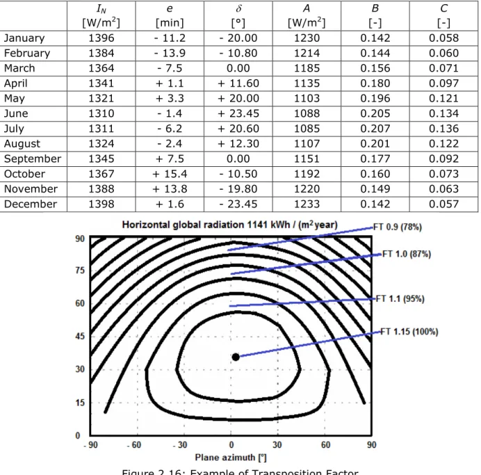
the generic surface of the building ...37 Figure 2.15: Usual definition of solar azimuth angle in a building simulation software....38 Figure 2.16: Example of Transposition Factor ...40 Figure 2.17: Example of solar radiation distribution over one year for the TRY
of Venice ...43 Figure 2.18: Example of architectural elements shading partially the building
envelope ...44 Figure 2.19: Solar charts for some locations: 20° latitude (A), 40° latitude (B),
60° latitude (C) ...44 Figure 2.20: Solar chart and shape of surrounding area ...45 Figure 2.21: Diagram expressing relationship between air temperature and absolute humidity ...46 Figure 3.1: Heat conduction in a general medium ...48 Figure 3.2: Heat conduction through a building element: from inner surface to outer surface (a) and from indoor temperature and outdoor temperature (b) ...50 Figure 3.3: Thermal bridge due to a corner: materials (a) and temperature
distribution (b) ...52 Figure 3.4: Thermal bridge due to a pillar: materials (a) and temperature
distribution (b) ...52
15
Figure 3.5: Example of thermal bridge: a section of the corner (a) and boundary
conditions for the simulation (b) ...53
Figure 3.6: Surface moisture problem in a thermal bridge ...54
Figure 3.7: Assumptions for determining the thermal field inside building elements containing pipes ...55
Figure 3.8: Problem of sinusoidal boundary condition(a) and temperature trend in the thickness of the semi-infinite medium (b) ...56
Figure 3.9: Electrical analogy for a multi-layer wall ...57
Figure 3.10: Scheme of finite difference technique in one dimension problems ...58
Figure 3.11: Scheme of finite element technique in one dimension problems ...60
Figure 3.12: Approximatio of the function F(τ) by means of the series of triangles Fj ...61
Figure 3.13: Example of shape of the response function Dj due to the triangular impulse Ω u ...61
Figure 3.14: Transfer functions for building elements not containing pipes ...62
Figure 3.15: The transfer functions inside a structure that contains embedded pipes...64
Figure 3.16: Response factors for tile covered radiant floor: from internal to outer surface (a), from internal to pipe surface (b), from pipe to outer surface (c) ...66
Figure 3.17: Example of response factors and modified response factors obtained for a typical tile covered radiant floor: from pipe to pipe surface (a), from internal to pipe surface (b), from pipe to outer surface (c) ...67
Figure 3.18: Example of comparison between FDM and response factor technique in terms of heat flow through the pipe surface [W/m2] due to 50°C sudden change in the surface temperature of the pipe (the inner and outer surface remain at constant temperature) ...68
Figure 4.1: Different possibilities of heat losses through the ground of the considered building (in grey) Source: [38] ...70
Figure 4.2: Correction of the U-value of a structure with heat loss through the ground as a function of the parameter B’ calculated via equation (4.9) Source: [38] ...71
Figure 4.3: Simplified assumption in the resistance-capacity model for a simplified system which considers the room and the envelope ...72
Figure 4.4: Room with small window ...73
Figure 4.5: Room with large window ...74
Figure 4.6: Temperature drop in the case of a room with a small window ...75
Figure 4.7: Temperature drop in the case of a room with a large window ...76
Figure 4.8: Heat losses and heat gains in an average day in winter period ...77
Figure 4.9: Heat losses and heat gains in an average day in summertime ...78
Figure 4.10: Heat flows to be considered on a generic surface of the room ...78
Figure 4.11: Thermal balance of the air in a room ...80
Figure 4.12: Vapour balance in a room ...82
Figure 4.13: Convective heat transfer coefficients calculated with equation (4.35) (floor heating), euquation (4.36) (wall heating), equation (4.37) (ceiling heating), equation (4.38) (floor cooling) and equation (4.39) (ceiling cooling), by considering an equivalent diameter of the surface De of 3 m ...83
Figure 4.14: Determination of the view factors between building elements ...84
Figure 4.15: Determination of the view factors by means of diagrams ...85
Figure 4.16: Transmission, sorption and reflection coefficients as a function of the incident angle ...85
Figure 4.17: Transmittance characteristics of different glazing systems with respect to wavelength ...86
16
Figure 4.18: Transmittance characteristics of different glazing systems with respect to
wavelength ...87
Figure 4.19: Thermal processes involved in the energy transmitted through a glazing surface ...88
Figure 4.20: Determination of the g factor ...91
Figure 4.21: Radiation processes in a general i-th glazing element ...92
Figure 4.22: Possible schemes for determining window thermal balance ...93
Figure 4.23: Vertical discretisation of a double skin facade ...94
Figure 4.24: Possible schemes for the thermal balance within a double skin facade ...94
Figure 4.25: Response of human eye to the visible solar radiation spectrum ...95
Figure 4.26: Identification of building elements that are subject to direct solar radiation ...98
Figure 4.28: Schematic of the thermal balance for a simplified model ... 100
Figure 4.29: Schematic of the distribution of solar radiation inside of the room in the detailed model ... 100
Figure 4.30: Simplified model for the conductive heat transfer in a structure containing pipes ... 102
Figure 4.31: Effect of solar radiation in winter time for a cold week in Venice ... 104
Figure 4.32: Effect of solar radiation in summer time for a warm week in Venice ... 105
Figure 4.33: Graphical view of a step-wise constant heat gain and related cooling load ... 106
Figure 4.34: Equivalent difference of temperature for a clear grey South wall (a) and attenuation factor for the solar radiation entering the room as a function of the thermal capacity of the room for a window facing South (b) ... 107
Figure 4.35: Storage factor for 10 hours internal gains in a room as a function of the thermal capacity of the room ... 108
17
1. INTRODUCTION
The goal of a building and related services is to ensure a proper energy performance, taking into account outdoor climatic and local conditions, as well as indoor climate requirements and cost-effectiveness.
For this purpose, it is very important to define the internal conditions in terms of indoor temperatures and rates of ventilation. At the same time the outdoor conditions are of extreme importance, leading to different design and operating decisions. For this purpose the first chapter of the present work focuses on these two aspects, since they usually are the boundary conditions to be set for solving a problem dealing with the energy of a building and of one of its components.
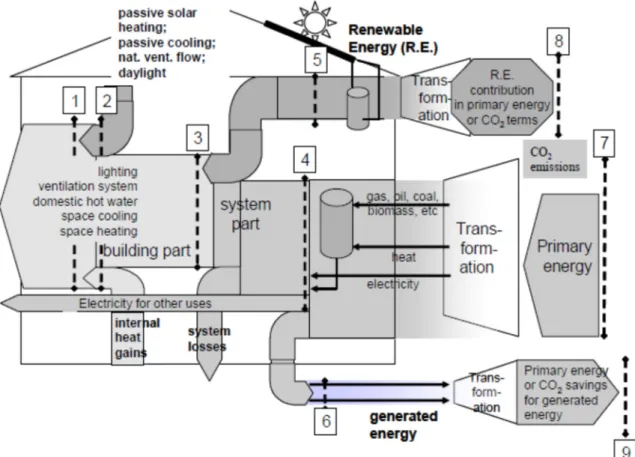
When looking at the energy performance of a building, the calculation for determining the primary energy consumption follows the scheme reported in Figure 1.1, as described by the umbrella document of CEN [1]. As can be seen, the energy flow goes from right-hand to left-hand; the energy calculation has to be performed the other way round from left- hand to right-hand. The present book deals with the section 3 reported in Figure 1.1, i.e.
the building energy need, without considering the heating, cooling and electric plants.
18
Figure 1.1: Energy flow chart for determining the primary energy consumption of a building
Source: [1]
It is evident therefore that it is extremely important to define properly the models dealing with the energy problems of the envelope for the different purposes. One of the most important physical phenomena in the building envelope is the heat transfer through conduction. For this reason the second chapter focuses on this subject. First the steady state problem in one-dimension and 2-dimensions is shown. Then the different solutions for the dynamic problem are shown, dealing with 1-dimension and 2-dimensions, with particular reference to building elements containing pipes, since they are used with increasing frequency in heating/cooling the buildings.
The last chapter of this book deals with the different energy models which can be used in determining problems related to energy in buildings. The first model shown is the steady state solution which is used for determining the peak heating capacity of a heating system. The second system shown is the resistance-capacity model which can be used for determining the constant time of a thermal system. Afterwards the quasi-steady state model is shown; it is one of the most common used, since it allows to determine the seasonal sensible heating and cooling demand of a building. As for the dynamic models, first the detailed heat balance model has been shown, with particular reference to the heat exchange coefficients to be used, as well as to the solar radiation through transparent components. Then thermal balance for rooms equipped with radiant systems are shown. Finally models based on the thermal response of the room are shown.
Very interesting problems are related to the use of natural ventilation [2, 3] or hybrid ventilation [4], or models with different air temperatures within a room [5], which can be
19
used in some particular cases. Despite the importance of these two problems, in the present work these two models are not shown, since the aim of the present book is to give the bases for the general approach of thermal modelling of a building and of its components.
20
2. INDOOR AND WEATHER CONDITIONS
2.1 Thermal comfort
2.1.1 Global thermal comfort conditions
The factors affecting the thermal comfort can be summarised as:
• air temperature
• surface temperatures
• air velocity
• relative humidity
• type of clothing
• activity level
Their influence has been widely studied and evaluation criteria such as PMV (Predicted Mean Vote, ranging between -3 for “very cold” and +3 for “very hot”) and PPD (Percentage People Dissatisfied) are nowadays of common use [6, 7, 8, 9]. The effect of the temperature of the different surfaces surrounding a person can be summarised by mean of a single quantity, the mean radiant temperature (tmr), which, in the case of radiantly grey surfaces with emissivities close to one can be expressed, in the absolute scale, as:
25 . 0
1
4 ,
⋅
=
∑
= − n k
k s k p
mr F T
T (2.1)
where Fp-k are the view factors between the human body and the surfaces and Ts,k their absolute temperatures; view factors can be determined by means of graphs [6] or, for computerised calculations, by means of algorithms based on spherical trigonometry [10].
Usually in building simulations the calculation of mean radiant temperature is carried out in a simplified way, by using the weighted average temperature on surface areas of the mean surface temperatures:
∑
∑
=
=
⋅
= n
k k n k
k s k mr
S T S T
1 1
,
(2.2)
21
The Fanger’s approach easily allows to predict users reactions (PMV and PPD), as a function of activity level (expressed by the metabolic rate M), clothing thermal resistance Rcl, mean radiant temperature tmr of the surrounding surfaces, as well as dry-bulb temperature ta, relative air velocity va and relative humidity of the air:
(
M t t R v RH)
f
PMV = , a, mr, cl, a, (2.3)
( )
[
0.03353 4 0.2179 2]
95
100 e PMV PMV
PPD= − ⋅ − ⋅ + ⋅ (2.4)
An important parameter, used in the study of thermal comfort, is the operative temperature to, which is a weighted value of air temperature ta and mean radiant tempe rature tmr, calculated as:
r c
mr r a o c
h h
t h t t h
+
⋅ +
= ⋅ (2.5)
where hc and hr are the convective and the radiant heat exchange coefficient between human body and the surroundings. If the air velocity is less than 0.2 m/s and the difference between the mean radiant temperature and the air temperature is less than 4°C, the operative temperature can be calculated, with a good approximation, as the average value between these two temperatures. The operative temperature is taken as a parameter involved in defining thermal comfort conditions in all the above mentioned standards.
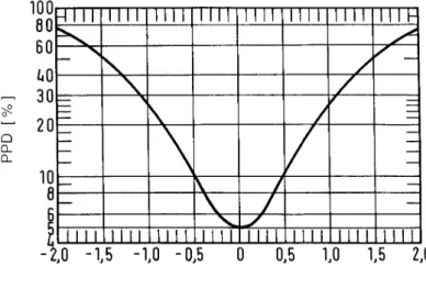
Figure 2.1: Percentage of people unsatisfied PPD as function of the predicted mean vote PMV
Source: [7]
2.1.2 Local discomfort conditions
There are some other parameters for comfort (namely local discomfort), which are the draft risk, the radiant asymmetry and the difference of temperature between head and feet.
If the air velocity is appreciable, the parameter DR (“Draft Risk”, expressed as percent of people dissatisfied due to draught) should be evaluated as well; in the following way:
22
(
t) (
v) (
v Tu)
DR= 34− a ⋅ a −0.050.62 ⋅ 3.14+0.37⋅ a⋅ (2.6)
where ta is the local air temperature, va is the local mean air velocity and Tu is the local turbulence intensity, defined as ratio between standard deviation and mean value of the local air velocity.
The radiant asymmetry is based on the definition of plane radiant temperature tpr, which is the temperature of a half-space defined by a horizontal plane, which can be evaluated as:
∑
= − ⋅= m
k
k s k p
pr F T
T
1
, (2.7)
where Fp-k is the view factor between a point of the plane and the surfaces of the half- space. The difference between the plane temperatures of the two half-spaces is the radiant asymmetry. The allowed values of this parameter are fixed in the current standards as the 5% of unsatisfied people. The curves defining the sensitivity of people to radiant asymmetry are reported in Figure 2.2.
Another parameter is the difference between air temperature at 0.1 m and air temperature at 0.6 m above the floor, in order to evaluate local discomfort: according to standards the value of this difference should be lower than 3°C.
Figure 2.2: Percentage of people dissatisfied as a function of the radiant asymmetry Source: [7]
2.1.3 Adaptive comfort conditions for unconditioned buildings
Adaptive comfort builds on the principle that people experience differently and adapt, up to a certain extent, to a variety of indoor conditions, depending on their clothing, their activity and general physical condition. Therefore, contrary to the conventional cooling which is based on pre-calculated temperatures and humidity levels, the adaptive approach is based on a non-fixed set of conditions, taking into account thermal perception and behaviour of the user, requiring him to take an active role in controlling his indoor environment [11].
23
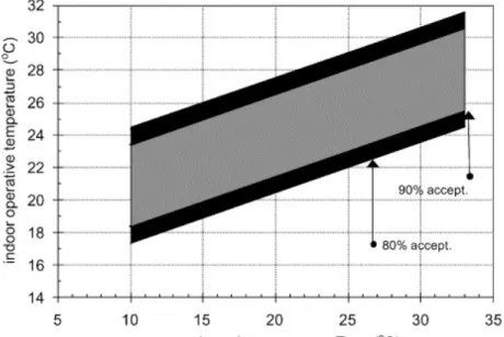
Based on this theory, currently two possible comfort criteria can be followed, as defined in the standards ASHRAE 55 [8] and EN 15251 [12]. They both give a range of acceptable indoor operative temperature according to outdoor temperature which has been shown to be the most important parameter affecting thermal comfort in unconditioned buildings. The difference in the two standards is the reference outdoor temperature, which is the monthly outdoor temperature in ASHRAE 55 (Figure 2.3) and the weekly mean running temperature in EN 15251 (Figure 2.4). These charts can be used both for previous calculations by means of dynamic simulations and for checking indoor environmental conditions with in situ measurements over a long period.
Figure 2.3: Acceptable range of operative temperature as function of the mean monthly outdoor temperature
Source: [8]
Figure 2.4: Acceptable range of operative temperature as function of the weekly running mean outdoor temperature
Source: [12]
24
2.2 Indoor Air Quality and ventilation requirements
Ventilating is the process of "changing" or replacing air in any space to provide high indoor air quality (i.e. to control temperature, replenish oxygen, or remove moisture, odors, smoke, heat, dust, airborne bacteria, and carbon dioxide). Ventilation is used to remove unpleasant smells and excessive moisture, introduce outside air, to keep interior building air circulating, and to prevent stagnation of the interior air.
There might be the following types of ventilations:
• Mechanical or forced ventilation: through an air handling unit or through the direct injection to a space by a fan and with an exhaust fan for the removal of air polluted by indoor contaminants (persons, furniture, chemical compounds, etc.), as shown in Figure 2.5a (balanced ventilation as defined by EN 12792 [13]).
Another possibility is to use either exhaust fans coupled with suitable openings in the window frames or on external walls, as shown in Figure 2.5b (exhaust ventilation as defined by EN 12792), or supply fans coupled with suitable openings in the window frames or on external walls, as shown in Figure 2.5c (supply ventilation as defined by EN 12792).
• Natural ventilation occurs when the air in a space is changed with outdoor air without the use of mechanical systems, such as a fan [14]. Most often natural ventilation is assured through operable windows: in this case it is usullay named single side ventilation (Figure 2.6a), but it would be more appropriate to name it airing. Natural ventilation usually has to be achieved by means of cross ventilation (Figure 2.6b) and through temperature and pressure differences between spaces, by means of stack effect inside the rooms (Figure 2.6c). Natural ventilation requires a proper design of the openings on the envelope of the building, taking into account the effects of the wind in terms of positive and negative pressures on the building itself and using the different natural ventilation strategies (Figure 2.6d).
• Mixed mode ventilation or hybrid ventilation: utilises both mechanical and natural ventilation processes. The mechanical and natural components may be used in conjunction with each other or separately at different times of day. The natural component is sometimes subject to unpredictable external weather conditions, hence it may not always be adequate to ventilate the desired space. The mechanical component is then used to increase the overall ventilation rate so that the desired internal conditions are met. Alternatively the mechanical component may be used as a control measure to regulate the natural ventilation process, for example, to restrict the air change rate during periods of high wind speeds in cold climates or when indoor conditions could reach high levels of operative temperature in warm climates.
• Infiltration is separate from ventilation. Infiltration is the unintentional or accidental introduction of outside air into a building, typically through cracks in the building envelope. Infiltration is sometimes called air leakage. Infiltration is caused by wind, negative pressurization of the building, and by air buoyancy forces known commonly as the stack effect.
The ventilation rate is normally expressed by the volumetric flowrate of outside air being introduced to the building. The typical units used are liters per second [l/s] or cubic meters per hour [m3/h]. The ventilation rate can also be expressed on a per person or per unit floor area basis, such as [l/(s person)] or [l/(s m2)], or as air changes per hour [h-1].
25
For residential buildings, which mostly rely on infiltration for meeting their ventilation needs, the common ventilation rate measure is the number of times the whole interior volume of air is replaced per hour, and is called air changes per hour (I or ACH) [h-1].
During the winter, ACH may range from 0.2 to 0.5 in a tightly insulated house to 0.8 to 1.5 in a loosely insulated house, depending on the outdoor weather conditions, e.g. wind speed and external temperature (the higher the temperature difference between indoor and outdoor the higher the infiltration rate). Recent studies have shown that a proper ventilation rate is at least 0.5 h-1 to reduce risks of asthma and allergy [15].
a b c
Figure 2.5: Mechanical ventilation using supply and an exhaust fans (a), using an exhaust fan and openings on the envelope (b) and using a supply fan and openings on
the envelope (c)
26
a b
c d
Figure 2.6: Natural ventilation using single side ventilation (a), cross ventilation (b), stack effect (c) and the combination of the different strategies (d)
Ventilation rates in commercial buildings may vary, depending on the acitivity and the required level of clearness. Usually a suitable value for achieving a proper ventilation rate is 10 l/(s person). In any case, for detailed analyses on the most suitable air flow rates the standards TR 14788 [16], EN 13779[17], EN 15251 [12] can be followed.
2.3 Climatic conditions
Weather is the state of the atmosphere, to the degree that it is hot or cold, wet or dry, calm or stormy, clear or cloudy. Most weather phenomena occur in the troposphere, just below the stratosphere. Weather refers, generally, to day-to-day temperature and precipitation activity, whereas climate is the term for the average atmospheric conditions over longer periods of time [18]. For energy uses in buildings weather conditions play an important role. For this reason it is important to define the proper boundary conditions in terms of the different parameters affecting energy and comfort in buildings, which may be different from case to case depending on the particular problem.
2.3.1 Outdoor temperature
Atmospheric temperature is a measure of temperature at different levels of the Earth's atmosphere. It is governed by many factors, including incoming solar radiation, humidity and altitude. When discussing surface temperature, the annual atmospheric temperature
27
range at any geographical location depends largely upon the type of biome, as measured by the Köppen climate classification (see Figure 2.7):
o GROUP A: Tropical/megathermal climates o GROUP B: Dry (arid and semiarid) climates o GROUP C: Temperate/mesothermal climates o GROUP D: Continental/microthermal climate o GROUP E: Polar climates
o GROUP H: Alpine climates
Nowadays climatic data are available for most of the climates. Weather conditions can be define by the following parameters:
• Design heating temperature
• Design cooling temperature
• Degree day
• Mean monthly temperatures
• Hourly values
• Test Reference Year
2.3.1.1 Design heating temperature
The design temperature for heating conditions is usually an extreme temperature which might occur in the heating season. Usually the design conditions assume a suitable number of days under constant climatic conditions, i.e. at the design temperature and with no solar radiation, so as to assume steady state conditions through the envelope. In the table 2.1 the dry-bulb temperatures corresponding to 99.6% and 99.0% annual cumulative frequency of occurrence of some World locations are reported. In the same table the month when the minimum temperature occurs is listed as well.
Figure 2.7: Köppen classification for climates Source: [19]
28 2.3.1.2 Design cooling temperature
The design temperature for cooling conditions is usually an extreme temperature which can occur in the cooling season. Usually the design conditions assume a suitable number of days repeating the same climatic conditions. The design day assumes a certain hourly profile of outdoor temperatures with clear sky conditions. In table 2.1 the dry-bulb temperature corresponding to 0.4%, 1.0%, and 2.0% annual cumulative frequency of occurrence and the mean coincident wet-bulb temperature of some World locations are reported. In the same table the month when the maximum temperature occurs is listed as well. The cyclic conditions of the design day can be calculated, once known the maximum temperature (Tamb,max) and the temperature difference between the minimum and maximum temperature (∆tamb) by means of the following equation:
amb h amb
h
amb t p t
t , = ,max − ∆ (2.8)
where ph is a coefficient depending on the considered time hour; its hourly value is listed in Table 2.2.
2.3.1.3 Degree day
The degree day is a value which determines immediately whether a climate is mild or cold. The degree day (DD) can be calculated considering the sum of the difference between the indoor temperature and the daily mean outdoor temperature tamb,d,j when the external temperature tamb,d,j<12°C, since it is commonly assumed that the heating system can be turned off if the average outdoor temperature is greater than 12°C. The equation defining the degree day is hence the following:
∑
=−
=365
1
,
, )
(
j
j d amb i t t
DD (2.9)
29
Table 2.1: Design winter and summer conditions of some cities around the World Heating coldest month Cooling hottest month
[n]
DB 99.6%
[°C]
DB 99.0%
[°C] [n]
DB Range
[°C]
DB 4%
[°C]
WB 4%
[°C]
Abu Dhabi 1 11.5 12.9 8 12.5 44.9 23.2
Athens 2 1.6 3.1 8 9.1 35.1 21.1
Auckland 7 1.8 2.9 2 6.9 25.2 19.7
Bangkok 12 19 20.4 4 9.2 37.2 26.7
Beijing 1 -10.8 -9.1 7 8.9 34.9 22.2
Berlin 2 -11.8 -10.8 7 9.2 30 18.9
Buenos Aires 7 -0.1 1.3 1 11.8 33.7 22.5
Cairo 1 7.7 8.7 7 11.5 38.1 21.1
Cape Town 7 3.8 5 2 9.5 31 19.4
Caracas 2 20.7 21.2 9 7.2 33.4 28
Chicago 1 -20 -16.6 7 10.5 33.3 23.7
Dakar 2 16.5 16.9 9 5.1 32.1 23.5
Debrecen 1 -13.8 -10.9 7 11.1 7.7 21.3
Helsinki 2 -22.8 -19.1 7 9.5 26.7 17.9
Houston 1 -1.6 0.5 7 10.1 36 24.8
Lima 8 14 14.6 2 6.3 29.3 23.6
London 2 -4.6 -3 7 9.7 27.2 18.7
Melbourne 7 2.8 3.8 2 11.6 34.6 18
Mexico City 1 4.1 5.6 5 13.8 29 13.8
Montreal 1 -23.7 -21.1 7 9.3 30 22.1
Moscow 2 -23.1 -19.8 7 8.3 28.4 20.1
Mumbai 1 16.5 17.8 5 5.6 35.8 23
Nairobi 7 9.8 11 3 11.9 29 15.7
New Delhi 1 6.3 7.3 6 9.7 42 22.2
New York 1 -10.7 -8.2 7 7.4 32.1 23.1
Paris 1 -5.9 -3.8 7 10.1 30.9 20.1
Phoenix 12 3.7 5.2 7 12 43.4 21.1
Riyadh 1 5.9 7.2 7 13.5 44.2 18.7
Salt Lake City 1 -12.6 -9.9 7 14.4 36.3 17.5
San Paulo 7 8.9 10 2 8.2 32.1 20.4
Seville 1 1.3 2.9 7 16.4 39.9 23.8
Sidney 7 6 7 2 6.5 32.8 19.6
Singapore 12 23 23.5 6 5.5 33.2 26.4
Stockholm 2 -17.8 -14.2 7 9.4 27.1 17.5
Strasburg 1 -9.8 -7 7 11.1 31.1 20.9
Tehran 1 -2.8 -1.3 7 10.6 38.5 19
Tokyo 1 -6.9 -5.1 8 7.7 32.1 26
Vancouver 12 -7 -4 8 7.6 25 18.2
Venice 1 -4 -2.8 7 8.8 31.1 23.5
Washington DC 1 -10.6 -8.2 7 10.4 34.4 23.9
30
Table 2.2: Values of ph coefficient to be used in equation (2.8) for each hour of the day
hour 1 2 3 4 5 6 7 8
ph 0.87 0.92 0.96 0.99 1 0.98 0.93 0.84
hour 9 10 11 12 13 14 15 16
ph 0.71 0.56 0.39 0.23 0.11 0.03 0 0.03
hour 17 18 19 20 21 22 23 24
ph 0.1 0.21 0.34 0.47 0.58 0.68 0.76 0.82
Usually the indoor reference indoor temperature is considered to be 20°C, but in some cases it could be considered lower than 20°C. The degree day can be calculated in a simpler way as the difference between the indoor temperature and the mean outdoor monthly temperature tamb,m,z times the number of days of the considered month nd,z:
( )
[ ]
∑
=⋅
−
= 12
1
, , , z
z d z m amb
i t n
t
DD (2.10)
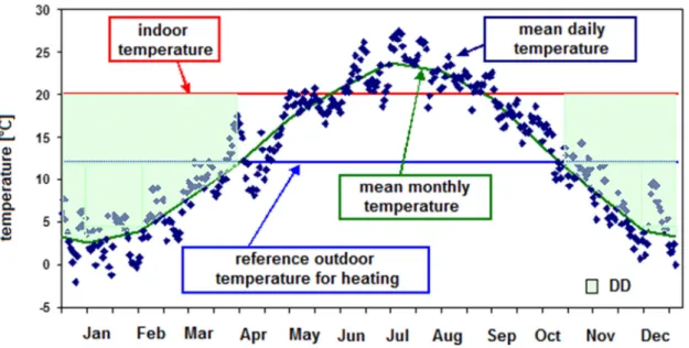
In Figure 2.8 the graphical meaning of the degree day is shown considering 20°C as reference indoor temperature. As can be seen the degree day is the light green area between the indoor temperature and the outdoor mean monthly temperature; the wider the green area (i.e. the higher the degree day), the colder the climatic conditions.
Sometimes, in order to check the potential of heating and cooling of a location, the degree days might be calculated for both winter and summer conditions, considering 18°C and 10°C as indoor temperatures. In Table 2.3 the values of heating and cooling degree days (DD) are reported for 18°C and 10°C as indoor temperatures.
Figure 2.8: Graphical representation of the Degree Days of a typical year in Venice
31
Table 2.3: Winter and summer degree days of some cities around the World
Heating DD Cooling DD
18°C 10°C 18°C 10°C
1 Abu Dhabi 24 0 6254 3358
2 Athens 1112 82 2966 1076
3 Auckland 1163 0 1909 131
4 Bangkok 0 0 6757 3837
5 Beijing 2906 1420 2199 765
6 Berlin 3156 1191 1125 170
7 Buenos Aires 1189 0 2524 663
8 Cairo 307 0 4472 1859
9 Cape Town 868 0 2388 326
10 Caracas 0 0 6002 3082
11 Chicago 3430 1748 506 1743
12 Dakar 1 0 5151 2231
13 Debrecen 3129 1313 279 1384
14 Helsinki 4721 2336 577 33
15 Houston 774 134 1635 3915
16 Lima 114 0 3541 735
17 London 2886 778 864 32
18 Melbourne 1733 127 1525 210
19 Mexico City 547 0 2503 131
20 Montreal 4493 2525 1185 234
21 Moscow 4655 2498 862 99
22 Mumbai 0 0 6219 3299
23 Nairobi 243 0 2870 193
24 New Delhi 278 0 5363 2721
25 New York 2627 1052 639 1984
26 Paris 2644 791 1209 142
27 Phoenix 543 28 2661 5066
28 Riyadh 305 0 5915 3301
29 Salt Lake City 2908 1200 669 1881
30 San Paulo 293 1 3483 854
31 Seville 927 19 3031 1020
32 Sidney 687 5 2871 634
34 Singapore 0 0 6374 3454
35 Stockholm 4239 1965 683 36
36 Strasburg 2947 1054 1162 136
37 Tehran 1749 577 1482 3230
38 Tokyo 2311 794 1911 508
39 Vancouver 3020 901 806 5
40 Venice 2262 762 1906 526
41 Washington DC 2478 993 730 2164
32 2.3.1.4 Mean monthly temperatures
Mean monthly temperatures define the mean temperatures of each month of the year.
They may be shown together with the maximum mean value and the minimum mean value of the month. In any case, for energy purposes the average outdoor temperature of the month is sufficient to determine many physical phenomena which may happen in a building.
As will be shown afterwards, the average outdoor temperatures may be used for evaluating the net energy demand of a building by means of the quasi-steady state method. The average value of outdoor temperature may be used also for determining the average water vapour content inside a building, as well as for checking moisture problems on internal surfaces of the envelope and interstitial condensation problems inside wall structures.
2.3.1.5 Profile of hourly average temperatures of the month
The profile of the hourly average temperatures of the month can be used for several purposes. It might be used for determining the energy demand of buildings for both heating and cooling.
If the monthly values are not known the hourly trend of temperatures can be built up by using the average values of the outdoor temperature and the mean values of minimum and maximum temperatures.
2.3.1.6 Test Reference Year
The Test Reference Year (TRY) is the hourly average profile of outdoor temperature of one typical year. The TRY is built up based on at least 20 years. The TRY is built up by calculating the mean outdoor temperature. The real occurred month which presents outdoor conditions which are the closest to the average value of the series is chosen to be representative of real conditions. Real hourly values over the month are used for building the TRY, since the combination of solar radiation and temperature may lead to errors in the evaluation of energy demand of the building. Therefore it is assumed that the most suitable trend of outdoor weather for determining the energy heating/cooling demands is based on real happened conditions. The use of artificial weather data may lead to mistakes, therefore, in case of few data for the climatic conditions, it is preferable to use average monthly data, instead of random profiles reconstructing TRY.
2.3.2 Solar radiation
The spectrum of the Sun's solar radiation is close to that of a black body with a temperature of about 5800 K. The shape of the spectrum of energy emitted by a body is expressed by the well-known Wien law which gives the peak in wavelength depending on the temperature of the radiative surface (Figure 2.9):
T 2898
max =
λ (2.11)
The Sun emits electromagnetical radiation across most of the electromagnetic spectrum, emitting X-rays, ultraviolet, visible light, infrared, and even Radio waves.