hjic.mk.uni-pannon.hu DOI: 10.33927/hjic-2020-14
EXAMINATION OF FUEL CONSUMPTION FACTORS, BASICS OF PRECI- SION AND ON-BOARD DIAGNOSTIC MEASUREMENTS
TIBOR BUSZNYÁK∗1 ANDISTVÁNLAKATOS1
1Department of Road and Rail Vehicles, Széchenyi István University, Egyetem tér 1, Gy ˝or, 9026, HUNGARY
In this paper, different factors of fuel consumption are examined. Driveload equitation is used as a basis and the parts that handle energy consumption in particular are analyzed. For the purposes of visibility, it was implemented using MAT- LAB. In statistical works, fuel consumption data require that the energy consumption of vehicles be analyzed correctly.
Variables which affect fuel consumption during a given drive are defined. Research is analyzed in the second part of the paper where vehicle diagnostics are combined with global positioning. Examinations are necessary to create on-board diagnostics-based positioning.
Keywords: GPS, OBD, correlation, drive, assistance
1. Introduction
Nowadays, innovation is a key. Economical, safety- centred or traffic optimization tasks are increasingly reg- ulated. These criteria require developers to actuate and consequently upgrade their conceptions. New technolo- gies are rapidly emerging so industries have to keep up to date. Drive options, including alternative drive solutions, are continuously being updated, the number of driver- assistance features is ever-increasing towards a possible fully autonomous level [1].
The role of development focusing on Smart City con- cepts and sustainable traffic is becoming more important.
Critical aspects of it are efficient energy use (the central question of the present paper), range of online communi- cation systems, autonomous transport systems and con- ceptions of autonomous vehicles. Reliable operation re- quires cooperation between different participants, e.g. the information technology, urban development and automo- tive industries. These aspects are interrelated, therefore, a more efficient Intelligent Transportation System (ITS) could be realized [2–4].
Information technologies between different units of traffic are elementary in terms of automated traffic.
The stability of dataflow is unavoidable. Communication channels play a key role in everyday life as information is accessed from the Internet.
As information content defines the quality of data, the demands of traffic quality have recently been increasing.
The number of automobiles in Hungary has almost doubled over the past twenty years. Safety issues and
∗Correspondence:busznyaktibor@gmail.com
accidents are increasingly commonplace. Besides acci- dents, traffic jams have also become more frequent.
As a result, driving has become harder. Rush-hour traffic that slowly inches forward, searching for a parking space or simply parking itself put drivers to the test un- der crowded, metropolitan conditions. The need to avoid similar situations has led to the emergence of driver- assistance systems.
The quality of data transmissions as well as trou- ble logger- and indicator systems, which evaluate in- puts from sensors or on-board diagnostics, are closely connected to vehicle information. The aforementioned technologies help driver-assistance systems to function.
Due to information technology and automatization, it is possible to create a vehicle network. One of these net- works is the vehicle-to-everything (V2X) communication platform where vehicles communicate with each other along with the infrastructure provider to share informa- tion about the locations of traffic jams and avoid conges- tion. Vehicle communication and driver-assistance sys- tems help to improve road traffic safety and make more accurate predictions [5–7]. An important task is to define databases based on the optimization of traffic.
Several methods, e.g. based on vehicles or infrastruc- ture, are available in order to build a database.
If the vehicle investigated predominantly drives in well-maintained, intelligent infrastructure, then the num- ber and complexity of built-in vehicle systems can be re- duced.
In this case, information is supplied to the vehicle by an uninterrupted connection with external systems. This could also be true of the drive of a vehicle on predefined routes, e.g. buses. It is easier to build infrastructure for
public transport vehicles because their routes are prede- fined. On the other hand, a vehicle can be defined as a sep- arate unit. Without infrastructure, vehicles rely on built-in sensors and can drive anywhere, external infrastructure is unnecessary.
How could the complexity of a given vehicle’s sensor system be reduced? Would it be possible to use built-in on-board diagnostics for positioning tasks.
Basic ideas originate from simple experiences. If peo- ple drive uphill in cruise control, the amount of data con- cerning fuel consumption that appears on the dashboard increases. The core of this research is the possible con- nection between elevation and fuel consumption:
1. Can a connection between elevation data from global positioning and fuel consumption data from on-board diagnostics at a constant or various speeds be identified?
2. Is it possible to create a topographic elevation model from fuel consumption data?
3. If it is possible, then the fuel consumption can be predicted from road conditions.
4. By integrating on-board diagnostics into conven- tional or intelligent transportation systems using the presented relations, a vehicle can be located.
Connections between data from global positioning sys- tems and fuel consumption are sought. It is necessary to define important variables that affect the fuel consump- tion of a vehicle. The relevant equations and propulsion power requirements are analyzed.
2. Experiment
2.1 Propulsion power requirements and fuel consumption – defining variables
Internal combustion engines function by burning fuel which is blended with air in line with energy require- ments. Propulsion power is necessary for a vehicle to move but its movement is restricted by various internal and external driving resistances.
External driving resistances Rolling resistance is
Fg=µmg (1)
The rolling force resists motion when tires are rotating on a given surface. Internal and external factors are included in the equation.
The external factor is the rolling resistance coefficient which depends on contacting surfaces. The internal factor is the deformation of the tires which is dependent on the load of the vehicle. A loss in power results. Power against rolling resistance is
Pg=Fgv (2)
Aerodynamic drag is
Fl=cwρAv2/2 (3) Drag acts in the opposite direction to which the vehicle is moving. It plays a major role in terms of vehicle dynam- ics and efficiency.
At higher speeds, it is more significant because drag increases with the square of the velocity. Power against drag is
Pl =Flv (4) Climbing resistance is
Fe=mgsin(α) (5) Climbing resistance depends on the elevation of the route, mass of the vehicle and road gradient. Power against climbing resistance is
Pe =Fev (6) Internal driving resistances
Acceleration resistance is
Fgy= (1 +θ)ma, (7) whereθis a coefficient of rotating components (Table 1).
Energy is required to accelerate. The acceleration resis- tance can be calculated from the masses of the rotating components and vehicle. Power against acceleration re- sistance is
Pgy =Fgyv (8) Other internal resistances, e.g. transmission resistance, are
Peff = (1−η)Ph (9) Another internal resistance arises when the transmission system moves and depends on the efficiency of its parts, moreover, it is used to calculate power.
This internal resistance is constant and includes the efficiency of the differential (0.93), efficiency of the clutch (0.99), efficiency of the drive shaft (0.99), effi- ciency of the gearbox (0.97) and efficiency of the bear- ings (0.98):
η=ηtkηdiffηktηcsηny (10) Finally, energy produced by the combustion of fuel is translated into the energy requirements of given resis- tances. At constant velocities, the acceleration resistance is zero and transmission resistance constant as well as cal- culable, as is shown inTable 2. Thus, the traction force or driveload equitation can be written in the following well- known form:
Fv =Fe+Fg+Fl (11) Pv =Fvv (12)
Table 1:Values ofθ Gear [ith] θ
1 0.4
2 0.3
3 0.2
4 0.1
5 0.08
Table 2:Defined variables Known values A,m,g,µ,cw,ρ Variables v,α
2.2 MATLAB implementation
The analysis of traction force components was conducted in the MATLAB development environment to try and define how variations in velocity and road gradient can explain power requirements. An analysis was conducted based on theoretical elements and data were defined by given measurements.
Vehicle: Ford B-Max (2014)
• empty mass (m) =1275kg;
• maximum power (Pmax,Peff) =74kW;
• drag coefficient (cw) =0.32;
• frontal area (A) =2.8m2;
• rolling coefficient (µ) =0.007 Velocity codomain:
• v= [0,140km/h]
Road gradient codomain:
• α= [0,30◦]
Figs. 1-3show the effects of different resistances. The rolling resistance diagram (Fig. 1) exhibits a linear trend.
The power demand increases as the velocity and road gra- dient increase. The climbing resistance diagram (Fig. 2) also exhibits a linear trend. According to real data, it is necessary to define a power limit, in this case 74 kW, which is the maximum power of the vehicle.
Analysis above this limit in not required since the en- gine is incapable of providing more power. On the con- trary, the vehicle would decelerate or remain stationary beyond this limit.
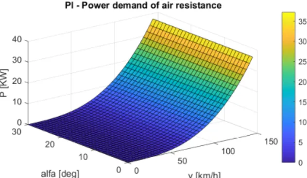
The air resistance diagram (Fig. 3) exhibits a square trend between the velocity and power demand of the ve- hicle.
The power demands of external resistances are pre- sented inFig. 4. Important values were compiled inTa- bles 3–5.
In the first part of this chapter, constant, discrete velocities were assumed. The next step is the parameter- ization of acceleration. For this task, values of theta are required (Table 1).
Acceleration codomain
Figure 1:Diagram of the power demand of rolling resis- tance as a function of velocity and road gradient
Figure 2:Diagram of the power demand of climbing re- sistance as a function of velocity and road gradient
Figure 3:Diagram of the power demand of air resistance as a function of velocity and road gradient
• a= [0,5m/s2]
Gravitational acceleration [G] is a dimensionless, unoffi- cial and descriptive measure.Gcodomain can be derived from a codomain.
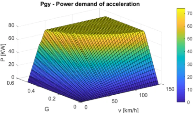
The effects of acceleration are shown inFig. 5. It is visible that at predefined shifts, diagram flow refracts and represents real cases. Important values are compiled in Tables 6–8.
3. Results and Analyses
At high velocities and on steep road gradients, the power demand is also higher. The declaration of variables is nec- essary as a result of precise planning to follow on-board diagnostics (OBD) measurements, especially routes. Two independent measurement systems, OBD and GPS, are
Figure 4:Diagram of the power demand of external resis- tances as a function of velocity and road gradient
comparable to connect the concept [8]. Precision posi- tioning is widely used and consists of numerous impor- tant boundary conditions. This paper examines the OBD side of the concept, details of precise GPS and GNSS measurements are presented in previous papers of ours.
A statistical analysis of the fuel consumption database is given from the equation of motion.
For this database, work was used, that is the product of the force and displacement in the direction of the force.
Table 3:Notations of v andαvariables v(↓) low velocities
v(←) medium velocities v(↑) high velocities α(↓) shallow road gradients α(←) medium road gradients α(↑) steep road gradients
Table 4:Values forP[v, α]calculated in the MATLAB environment
v(↓)= 3.6 [km/h]
α(↓) = 0◦ P= 0.3064 [kW]
α(←)= 5◦ P= 1.178 [kW]
α(↑)= 30◦ P= 6.342 [kW]
v(←)= 50 [km/h]
α(↓) = 0◦ P= 2.824 [kW]
α(←)) = 5◦ P= 18.09 [kW]
α(↑)= 30◦ P= 74 [kW]
v(↑)= 140 [km/h]
α(↓) = 0◦ P= 40.78 [kW]
αmax(140) = 4◦ P= 74 [kW]
α(↑) =α(←) =αmax
Table 5:P[v, α]matrix
P[v, α] v(↓) v(←) v(↑) α(↓) P(↓) P(↓) P(←) α(←) P(↓) P(←) P(↑) α(↑) P(←) P(↑) P(↑)
Figure 5:Diagram of the power demand of acceleration as a function of velocity andG
Lifting work is
Wem=Fem∆s=mg∆h (13) Lifting work is the work that is done by lifting an object over a given period of time. It is proportional to its mass and change in height.
Friction (or rolling) work is
Ws=µmg∆s (14)
Table 6:Notation ofvandGvariables v(↓) low velocities
v(←) medium velocities v(↑) high velocities G(↓) low accelerations G(←) medium accelerations G(↑) high accelerations
Table 7:Values for P[v, G]calculated in the MATLAB environment
v(↓)=3.6 [km/h]
G(↓)=0.01 P=0.1785[kW]
G(←)=0.1 P=1.185[kW]
G(↑) = 0.3 P = 5.93[kW]
v(←)=50 [km/h]
G(↓)=0.01 P=2.142[kW]
G(←)=0.1 P=21.42[kW]
G(↑)=0.3 P=64.26[kW]
v(↑)=140 [km/h]
G(↓)=0.01 P=5.508[kW]
Gmax(140)=0.1424 P=74[kW]
G(↑)=G(←)=Gmax
Table 8:P[v, G]matrix
P[v, G] v(↓) v(←) v(↑) G(↓) P(↓) P(↓) P(←) G(←) P(↓) P(←) P(↑) G(↑) P(←) P(↑) P(↑)
Table 9:Proportionalities over the period of time
Wem v,∆h Ws v Wgy v2 Wk v2
Table 10:Determination of coefficients Constant veloc-
ity [km/h]
Coefficient of deter- mination [R2]
30 0.9549
40 0.9160
50 0.8370
Friction work is proportional to its mass and displace- ment.
Acceleration work is Wgy=1
2m∆v2 (15)
Acceleration work is proportional to its displacement, mass and the square of its velocity.
Work done by air resistance is Wk= 1
2Acwρv2∆s (16) Work done by air resistance is proportional to its dis- placement, drag coefficient (cw), frontal area (A), density (ρ) and square of its velocity. For the purpose of statistical analysis, proportionalities were compiled inTable 9.
Now the statistical analysis can be conducted. In the first step, a single variable analysis is carried out. Previ- ously, a given route was measured, thus GPS and OBD databases were available. A connection between eleva- tion and fuel consumption data was sought.
Table 10 shows that the concept is highly usable at low velocities, but when the range of velocities increases, the coefficient of determination becomes less efficient.
Multivariate analysis provides a solution to this prob- lem. In this case, experienced variables, as summarized in Table 9, were used. A route comprised of different road gradients and velocities was examined.
A visual check is recommended to summarize the regression model, with which it is possible to forecast correlations according to different predictors (R2).
Range of velocity = [20, 70 km/h]
1. Examination with∆(v2)
• R2= 57.2%
• where∆(v2)= variation in the square of the velocity.
2. Examination with∆(v2)and∆h
Figure 6:Results of the multivariate analysis
• R2= 86.4%
• where∆h= change in height.
3. Examination with∆(v2),∆handv
• R2= 87.1%
• wherev= actual velocity.
Fig. 6respresents the regression equation with the co- efficient of determination.
The regression equation can be rewritten in the fol- lowing form:
Con=A∆(v2) +B∆h+Cv+D (17) Conis an abbreviation of fuel consumption and appears constant. It reflects other possible predictors that have not been examined, for example, losses of the internal com- bustion engine.
3.1 OBD-based positioning
A drawback of precision positioning devices on the mar- ket are their prices, but the OBD connectors are basic, standardized accessories of vehicles. The presented struc- ture, when a connection is made between the positioning and on-board diagnostics, can be used for driver assis- tance tasks [9].
A MATLAB implementation of OBD-based position- ing has been proposed that is connected to the aims of this paper and will be presented shortly.
Dataflow and the stability of the system with regard to a precision positioning measurement are crucial. Its boundary conditions are the following:
• Connection to 5 GNSS satellites simultaneously;
• Dataflow stability in terms of the satellites and the base;
• Online connection with the base, from where the correction of data originates.
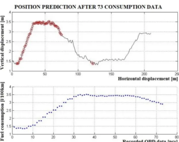
Figure 7:Operation of the MATLAB algorithm for OBD- based positioning
While weighing up the risks of two independent measure- ment methods, it is clear that the precision positioning technique is riskier.
A significant safety risk can be reduced if it can be substituted for other alternatives. An alternative to the el- evation database of the routes and OBD data, which is accessible to every vehicle, may exist.
To summarize our MATLAB implementation, contin- uously incoming OBD data are compared to a reference database which consists of a map with coordinates.
By searching for the minima of the squared differ- ences of the two databases, an algorithm was derived that is capable of defining position based on changing trends.
Fig. 7 presents the operation of the developed algo- rithm at a constant velocity of 30 km/h. Few incorrect OBD data points were obtained, for example, at a hor- izontal displacement of 125 m. As the database of fuel consumption is continuously expanding, the significance of this imprecision is decreasing.
4. Conclusion
In this article, the driveload equitation was examined and special care taken with regard to its power demands. In the MATLAB environment, characteristics of different resistances were shown. Moreover, the fixing of depen- dent variables was the main exercise in this research be- sides understanding the basic connections between on- board diagnostics and precision positioning. OBD-based positioning is a possible method to determine the actual position of a vehicle without constantly being connected to GPS or GNSS. It could be useful as part of V2X or other intelligent transportation systems. In order to ex- tend the concept to electric vehicles, the velocity and road gradient are the main variables, the power demands of both are comparable, and optimal charging points on a given route can be calculated. This could form the basis for a future paper.
Symbols
µ rolling resistance coefficient m mass of moving object g gravitational acceleration v velocity
cw drag coefficient
ρ density
A front surface α road gradient
θ coefficient of rotating object a acceleration
G gravitational constant η efficiency
ηtk efficiency of gearbox ηdiff efficiency of the differential ηkt efficiency of cardan-shaft ηcs efficiency of bearings ηny efficiency of the clutch h altitude
s displacement
Acknowledgements
This research was carried out as part of the EFOP- 3.6.2-16-2017-00016 project within the framework of the New Széchenyi Plan. The completion of this project was funded by the European Union and co-financed by the European Social Fund.
REFERENCES
[1] Takács, Á.; Rudas, I.; Bösl, D.; Haidegger, T.: Highly Automated Vehicles and Self-Driving Cars, IEEE Robotics & Automation Magazine, 2018,25(4), 106–
112DOI: 10.1109/MRA.2018.2874301
[2] Derbel, O.; Peter, T.; Zebiri, H.; Mourllion, B.;
Basset, M.: Modified intelligent driver model for driver safety and traffic stability improvement,IFAC Proceedings Volumes, 2013, 46(21), 744–749 DOI:
10.3182/20130904-4-JP-2042.00132
[3] Iordanopoulos, P.; Mitsakis, E.; Chalkiadakis, C.:
Prerequisites for Further Deploying ITS Systems:
The Case of Greece, Periodica Polytechnica Trans- portation Engineering, 2018, 46(2), 108–115 DOI:
10.3311/PPtr.11174
[4] Lim, C.; Kim, K.; Maglio, P. P.: Smart cities with big data: Reference models, challenges, and considerations, Cities, 2018, 82, 86–99 DOI:
10.1016/j.cities.2018.04.011
[5] Omae, M.; Fujioka, T.; Hashimoto, N.; Shimizu, H.:
The application of RTK-GPS and Steer-by-wire tech- nology to the automatic driving of vehicles and an evaluation of driver behavior,IATSS Research, 2006, 30(2), 29–38DOI: 10.1016/S0386-1112(14)60167-9
[6] Péter, T.; Bokor, J.: Modeling road traffic networks for control,Annual International Conference on Net- work Technology & Communications: NTC 2010, 2010, Paper 21, 18–22ISBN: 978-981-08-7654-8
[7] Péter, T.; Bokor, J.: New road traffic networks models for control,GSTF International Journal on Comput- ing, 2011,1(2), 227–232DOI: 10.5176/2010-2283_1.2.65
[8] Sun, Q.; Xia, J.; Foster, J.; Falkmer, T.; Lee, H.: Pur- suing Precise Vehicle Movement Trajectory in Urban Residential Area Using Multi-GNSS RTK Tracking, Transportation Research Procedia,2017,25, 2356–
2372DOI: 10.1016/j.trpro.2017.05.255
[9] Busznyák, T.; Pálfi, G.; Lakatos, I.: On-Board Diagnostic-based Positioning as an Additional In- formation Source of Driver Assistant Systems,Acta Polytechnica Hungarica, 2019, 16(5), 217–234ISSN:
1785-8860