Brain Tumor Detection and Segmentation from Magnetic Resonance Image Data Using Ensemble Learning Methods
Agnes Gy˝orfi, Levente Kov´acs and L´aszl´o Szil´agyi´
Abstract— The steadily growing amount of medical image data requires automatic segmentation algorithms and decision support, because at a certain time, there will not be enough human experts to establish the diagnosis for every patient. It would be a good question to establish whether this day has already arrived or not. Computerized screening and diagnosis of brain tumor is an intensively investigated domain, especially since the first Brain Tumor Segmentation Challenge (BraTS) organized seven years ago. Several ensemble learning solutions have been proposed lately to the brain tumor segmentation problem. This paper presents an evaluation framework de- signed to test the accuracy and efficiency of ensemble learning algorithms deployed for brain tumor segmentation using the BraTS 2016 train data set. Within this category of machine learning algorithms, random forest was found the most appro- priate, both in terms of precision and runtime.
Index Terms— magnetic resonance imaging, brain tumor, tumor detection, image segmentation, machine learning.
I. INTRODUCTION
Multi-spectral magnetic resonance imaging (MRI) is the medical imaging modality usually employed in brain tu- mor detection and segmentation [1]. The automatic brain tumor detection algorithms have intensively evolved as a consequence of the BraTS Challenges organized jointly with the MICCAI conference since year 2012 [2], [3]. A wide variety of algorithms were published that cover the whole methodology arsenal of pattern recognition. Most solutions employed supervised and semi-supervised machine learning techniques and/or advanced image segmentation tools like:
ensemble of random forests [4], AdaBoost classifier [5], random forests [6], [7], [8], extremely random trees [9], support vector machines [10], convolutional neural network [11], [12], deep neural networks [13], [14], [15], Gaussian mixture models [16], [17], fuzzyc-means clustering in semi- supervised context [18], [19], tumor growth model [20], and various advanced image segmentation techniques like cellu- lar automata combined with level sets [21], active contour models combined with texture features [22], and graph cut
*This project has received funding from the European Research Council (ERC) under the European Unions Horizon 2020 research and innovation programme (grant agreement No 679681). The work of L. Szil´agyi was supported by the Hungarian Academy of Sciences through the J´anos Bolyai Fellowship program.
All three authors are with University Research, Innovation, and Service Center (EKIK), Obuda University, B´ecsi ´ut 96/b, H-1034 Budapest,´ Hungary (phone/fax: +36-1-666-5585; e-mail: gyorfi.agnes at phd.uni-obuda.hu, {kovacs.levente,
szilagyi.laszlo} at nik.uni-obuda.hu).
A. Gy˝orfi and L. Szil´agyi are also with Dept. of Electrical En-´ gineering, Sapientia University, Calea Sighis¸oarei 1/C, 540485 Tˆırgu Mures¸, Romania (phone: +40-265-206-210; fax: +40-265-206-211; e-mail:
{gyorfiagnes,lalo} at ms.sapientia.ro).
algorithm [23]. Earlier solutions given for the brain tumor segmentation problem were summarized by Gordillo et al.
in [24].
This paper presents an evaluation framework designed to test machine learning algorithms in localizing brain tumors in MRI data provided by the BraTS challenges. In this study we compare the accuracy and efficiency of several ensemble learning techniques, placed into the same scenario, working with the same pre-processed data. The rest of the paper is structured as follows: section II presents the framework with its technical details (II-A) and the algorithms included in the evaluation (II-B). Section III provides a detailed analysis of the obtained results. Section IV concludes the study.
II. MATERIALS AND METHODS A. Framework
1) Data: All fifty-four low-grade (LG) tumor volumes of the BraTS 2016 train dataset [2] were involved in this study.
The multi-spectral MRI data contains four data channels (T1, T2, T1C, FLAIR). All volumes consist of 155 slices of 240×240pixels. Pixels are isovolumetric, each representing one cubic millimeter of brain tissue. Each volume contains approximately 1.5 million pixels. Human expert made anno- tation is available for each volume, making it possible to use these volumes as train and test data. All data channels were registered to T1 using an automatic procedure.
2) Processing steps: The block diagram of the application is presented in Figure 1. All data volumes went through a preprocessing step, which included histogram normalization and feature generation. After dividing the volumes into train and test data, train data is sampled for the ensemble learning, which is fed to the training algorithm. The trained ensembles are evaluated using the test data. The prediction provided by the ensemble is post-processed to give the tumor a regularized shape of improved quality. Finally, the accuracy of the algorithm is evaluated using statistical measures.
3) Pre-processing: Pre-processing theoretically has the main goal to deal with: (1) the intensity non-uniformity of the MR image volumes [25], [26], [27]; (2) the great variety of MR image histograms; (3) generating further features.
We have chosen to work with data that contain no visible inhomogeneity, the LG volumes of the BraTS 2016 train dataset [2], so no compensation is required. On the other hand, we produce uniform histograms to each data channel of the volumes using a context dependent linear transform that assigns the 25 and 75 percentile to intensity levels 600 and 800, respectively, and cuts the two tails of the transformed histogram at 200 and 1200. Details of this technique can 2019 IEEE International Conference on Systems, Man and Cybernetics (SMC)
Bari, Italy. October 6-9, 2019
Statistical evaluation
Morphological post−processing
Prediction by ensemble Preprocessing :
histogram normalization feature extraction
Train data sampling for ensemble learning
Training the selected ensemble
- -
-
? MRI
data
Dicescores
Fig. 1. Block diagram of the evaluation framework.
be found in our previous paper [28]. Besides the four observed data channels, 13 further features are generated, which were selected in a previous study [29] out of 100 generated morphological, gradient, and Gabor features. The 13 computed features used in this study include:
• nine features computed in 3×3×3 sized volumetric neighborhood: minimum of T1; minimum, average and maximum of T2; average and maximum of T1C; mini- mum, average and maximum of FLAIR intensity;
• three features extracted from 11×11 planar neighbor- hood: average of T2, T1C, and FLAIR intensities;
• and the average of FLAIR intensity obtained from3×3 planar neighborhood.
The final feature vector consists of 13 features, as the four observed features were finally excluded [29].
4) Decision making: The total number of 54 MRI vol- umes were divided arbitrarily into two equal groups. These groups served as train and test data in a two-round cross validation. This way we obtain a segmentation accuracy for each MRI volume using ensembles trained with volumes from the other group. Each unit in an ensemble was trained using the feature vectors of 10000 randomly selected pixels from the train volumes, out of which 92% were negative and 8% were positives. These percentages were decided based on previous studies [28]. All classifiers were trained to perform two-class separation, to distinguish normal tissues from tumor lesions.
5) Post-processing: The post processing step reclassifies each pixel based on the number of predicted positives situated within a cubic neighborhood. LG tumor volumes of the BraTS data set give best results using 11×11×11 sized neighborhood and threshold around 35% [28].
6) Evaluation criteria: Statistical evaluation is performed, which is based on the number of true positives (TP), true negatives (TN), false positives (FP), and false negatives (FN).
Accuracy indicators derived from these numbers, namely the Dice score (DS), sensitivity (true positive rate, TPR), speci- ficity (true negative rate, TNR), and accuracy (ACC), are exhibited in Table I. Each of these are extracted for individual volumes, while overall accuracy is expressed by the average and median values obtained for the 54 volumes. Further on, the average runtime of a single-volume segmentation is the main evaluation criterion of the speed.
TABLE I
CRITERIA TO EVALUATE SEGMENTATION QUALITY
Indicator Values
Name Formula Possible Ideal
Dice score DS =2×TP+FP+FN2×TP 0≤DS≤1 1
Sensitivity TPR =TP+FNTP 0≤TPR≤1 1
Specificity TNR =TN+FPTN 0≤TNR≤1 1
Accuracy ACC = TP+FP+TN+FNTP+TN 0≤ACC≤1 1
B. Algorithms
Ensemble learning methods use sets of weak classifiers to produce improved accuracy via majority voting. The algorithms involved in this study are:
• Random forest (RF) classifier, using the implementation given in OpenCV ver. 3.4.0. RF represents an ensem- ble of decision trees. The main parameter, beside the number of trees, is the maximum depth of each tree.
Experiments showed that train data sets of 10000 items were best learned using the maximum depth set to 7.
• Ensemble of real Adaboost classifiers, using the imple- mentation given in OpenCV ver. 3.4.0.
• Ensemble of artificial neural networks (ANN), using the implementation given in OpenCV ver. 3.4.0. Each ANN had the same architecture: input layer of size that corresponds to the number of features, two hid- den layers of 7 and 5 neurons, respectively, and one neuron in the output layer. ANNs were trained using the backpropagation rule implemented in OpenCV.
• Ensemble of binary decision trees (BDT), using an own implementation presented in [28]. BDTs can learn to perfectly separate negative from positive train samples unless there are two coincident vectors with different ground truth. Training sets of randomly chosen 10000 samples are usually learned by BDTs of maximum depth 19.3±3.6 (AVG±SD). Decisions are made at average depth of7.29±2.67.
III. RESULTS AND DISCUSSION
All the above mentioned algorithms underwent a thorough evaluation process involving the 54 low-grade tumor volumes of the BraTS 2016 database. The size of the ensemble varied in four steps, using values of 5, 25, 125, and 255. The
TABLE II
STATISTICAL ACCURACY INDICATOR VALUES OBTAINED FOR VARIOUS CLASSIFIERS AND ENSEMBLE SIZES. THE BEST ACHIEVED PERFORMANCE IS HIGHLIGHTED IN EACH COLUMN.
Classifiers Ensemble Dice score Sensitivity Specificity Accuracy
in ensemble size average median average median average median average median ANN
5 79.60% 83.57% 83.36% 86.77% 98.39% 98.78% 97.37% 97.61%
25 80.53% 84.39% 82.39% 85.75% 98.60% 98.92% 97.51% 97.79%
125 80.52% 84.07% 81.47% 85.20% 98.70% 98.92% 97.54% 97.84%
255 80.55% 83.99% 81.54% 84.93% 98.69% 98.94% 97.53% 97.78%
Adaboost
5 80.20% 84.28% 80.63% 85.46% 98.85% 99.03% 97.63% 97.74%
25 80.55% 84.13% 80.96% 86.68% 98.86% 99.12% 97.65% 97.76%
125 80.76% 84.11% 81.38% 86.96% 98.84% 99.11% 97.66% 97.87%
255 80.78% 84.13% 81.44% 87.00% 98.83% 99.10% 97.66% 97.85%
5 80.02% 82.94% 80.39% 83.38% 98.79% 99.03% 97.57% 97.90%
Random 25 81.10% 84.44% 81.90% 86.63% 98.78% 98.98% 97.67% 98.01%
forest 125 81.33% 84.36% 82.84% 87.31% 98.73% 98.93% 97.69% 97.71%
255 81.29% 84.32% 82.72% 87.35% 98.74% 98.93% 97.68% 97.72%
5 78.83% 83.59% 81.50% 85.80% 98.51% 98.86% 97.37% 97.53%
Binary 25 80.13% 83.83% 81.17% 84.72% 98.75% 98.95% 97.57% 97.59%
decision trees 125 80.21% 84.25% 81.41% 87.30% 98.75% 98.93% 97.56% 97.70%
255 80.22% 84.21% 81.44% 87.20% 98.75% 98.92% 97.57% 97.69%
TABLE III
COMPARISON OF CLASSIFIER ALGORITHMS USING THEDICE SCORES OBTAINED FOR THE54INDIVIDUALLGTUMOR VOLUMES. THE BEST ACHIEVED PERFORMANCE IS HIGHLIGHTED IN EACH ROW.
Classifier ANN Adaboost Random forest Binary decision trees
Ensemble size 5 25 125 255 5 25 125 255 5 25 125 255 5 25 125 255
DS>50% 52 52 52 52 52 51 51 51 51 51 53 52 51 52 52 52 DS>60% 50 50 50 50 50 50 51 51 50 51 51 51 48 48 49 49 DS>70% 45 45 47 47 45 44 45 45 44 47 48 48 42 46 45 46 DS>75% 41 43 43 43 41 42 42 42 43 41 41 41 40 42 41 41 DS>80% 38 37 37 37 39 40 40 40 39 40 40 40 34 36 37 37 DS>85% 19 24 24 22 24 22 24 24 20 25 24 25 22 22 23 24 DS>90% 5 8 8 7 7 10 10 10 12 10 10 10 8 8 7 7
LG tumor records in increasing order of statistical indicators
0 6 12 18 24 30 36 42 48 54
Statistical indicators (%)
30 40 50 60 70 80 90 100
Dice score Sensitivity
(a)
Fig. 2. Dice score and Sensitivity values obtained for each of the 54 LG tumor volumes using the random forest algorithm in ensemble of 125, plotted in increasing order of the quality indicators.
quality indicators exhibited in Table I were extracted for each scenario and each individual MRI record. The average and median value for each indicator was established for overall quality characterization. The algorithms were compared in group and one against one, through tests performed with individual data volumes and extracted overall quality bench- marks. Results are exhibited in the following.
Table II presents the global average and median values for all four quality indicators, obtained using the four evaluated classification algorithms and the above mentioned four en-
LG tumor records in increasing order of statistical indicators
0 6 12 18 24 30 36 42 48 54
Statistical indicators (%)
86 88 90 92 94 96 98 100
Specificity Accuracy
(b)
Fig. 3. Specificity and Accuracy values obtained for each of the 54 LG tumor volumes using the random forest algorithm in ensemble of 125, plotted in increasing order of the quality indicators.
semble sizes. The median values are always greater then the average, since there are a few data records of reduced quality that are usually segmented much worse than all others. The best values, which are highlighted in each column, suggest that the random forest performed slightly better than any other tested algorithm. Segmentation quality rises together with the size of the ensemble up to 125 units, and seems to saturate above this value. Best achieved average Dices scores are slightly above 81%, while median values approach 85%.
The accuracy of all algorithms is around 97.5%, meaning that
TABLE IV
DICE SCORE TOURNAMENT USING THE54 LGVOLUMES:ALGORITHMS AGAINST EACH OTHER,EACH USING ENSEMBLES OF SIZE125. HERE
ANNPROVED TO BE THE WEAKEST.
Algorithm ANN Adaboost RF BDT Won:Lost
ANN N/A 23:31 24:30 26:28 0:3 (73:89)
Adaboost 31:23 N/A 22:32 30:24 2:1 (83:79)
RF 30:24 32:22 N/A 25:29 2:1 (87:75)
BDT 28:26 24:30 29:25 N/A 2:1 (81:81)
about one pixel out of 40 is misclassified by these algorithms.
Figures 2 and 3 present the Dice score and Sensitivity, respectively the Specificity and Accuracy indicator values obtained by the most accurately performing ensemble of 125 random forests, evaluated on the 54 individual LG volumes. Apparently there are approximately 10% of the records that lead to mediocre result. In these cases the classification algorithm did not succeed to capture the main specific features of the data, probably due to the reduced quality of the recorded images.
Table III presents for each algorithm the number of records that led to Dice scores over predefined threshold values between 50% and 90%. The best values highlighted in each row of the table indicate again that random forest achieved the best segmentation quality, followed by Adaboost and ANN.
Figure 4 exhibits in a different format the Dice scores obtained by each algorithm using ensembles size of 125 units, tested on each individual LG tumor volume. Each graph presents the Dice scores obtained by two algorithms, plotted one against the other. Each cross (×) in these graph shows the Dice score of the two algorithms achieved on the very same data. Most crosses on each graph are close to the diagonal, indicating that the Dice score achieved by both algorithms were pretty much the same, but there are also crosses far from the diagonal, showing cases when one of the algorithms produced significantly better segmentation quality.
Table IV exhibits the same data as Fig. 4, but in a tournament format. Surprisingly, this table suggests that ANN is the worst performing algorithm in term of accuracy, because all other three classification methods achieved better Dice score in case of the majority of the data records. Again in this case, random forest proved the most accurate one, despite losing the direct comparison to BDT.
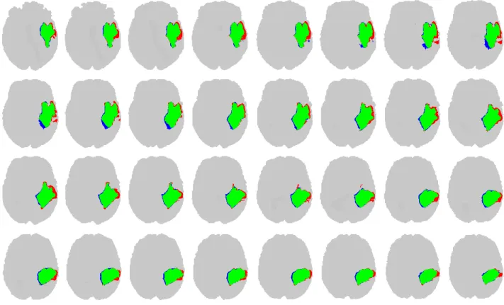
Figure 5 presents 32 subsequent slices from a segmented volume, obtained by the random forest composed of 125 trees. The algorithm finds the tumors pixels and also the boundary of the tumor with a good accuracy. True positives are drawn in green, false negatives in red, and false positives in blue color.
Figure 6 exhibits the efficiency benchmarks of the four algorithms. When we get a new data record of average size, we need to extract the 13 features for each pixel from its neighborhood, feed the obtained data to ensemble of classification algorithms of the chosen size, and finally apply
Dice score of ANN (%) 30 40 50 60 70 80 90 100
Dice score of Adaboost (%)
30 40 50 60 70 80 90 100
Dice score of ANN (%) 30 40 50 60 70 80 90 100
Dice score of RF (%)
30 40 50 60 70 80 90 100
Dice score of ANN (%) 30 40 50 60 70 80 90 100
Dice score of BDT (%)
30 40 50 60 70 80 90 100
Dice score of Adaboost (%) 30 40 50 60 70 80 90 100
Dice score of RF (%)
30 40 50 60 70 80 90 100
Dice score of Adaboost (%) 30 40 50 60 70 80 90 100
Dice score of BDT (%)
30 40 50 60 70 80 90 100
Dice score of RF (%) 30 40 50 60 70 80 90 100
Dice score of BDT (%)
30 40 50 60 70 80 90 100
Fig. 4. Dice scores obtained for individual volumes by the four algorithms using ensembles of size 125, plotted one algorithms vs. another, in all possible six combinations.
the post-processing that leads to final segmentation. The total necessary processing time, needed by each algorithm is shown in the figure. All tests were executed on a notebook computer with quad-core i7 processor running at 3.4GHz, using a single core of the microprocessor. Ensembles of RF and BDT performed quickly, in virtually same time. ANN and Adaboost required 2 to 5 times longer execution time, especially in larger ensembles.
IV. CONCLUSIONS
This paper presented a testing framework for ensemble learning algorithms, which were employed in brain tumor segmentation based on multispectral MR image data. The accuracy indicators showed, that all four tested algorithms are suitable to serve the decision making part of a segmen- tation procedure. The small differences in accuracy, and the runtime benchmarks suggest that the best solution from the tested ensemble learning algorithms is the random forest.
Further works will aim at including more machine learning algorithms into the framework.
Fig. 5. Thirty-two consecutive slices of a LG tumor volume, indicating true positive (green), false positive (blue) and false negative (red) pixels.
ANN Adaboost RF BDT
Average runtime (sec)
0 15 30 45 60 75 90 105 120 135 150 165
180 Average runtime of single-volume segmentation
Ensemble of 5 Ensemble of 25 Ensemble of 125 Ensemble of 255
Fig. 6. Efficiency benchmarks of the four classification algorithms: the average value of the total processing time in a single record testing problem.
REFERENCES
[1] G. Mohan and M. Monica Subashini, “MRI based medical image analysis: Survey on brain tumor grade classification,” Biomed. Sign.
Proc. Contr., vol. 39, pp. 139–161, 2018.
[2] B. H. Menze, A. Jakab, S. Bauer, J. Kalpathy-Cramer, K. Farahani, J. Kirby et al., “The multimodal brain tumor image segmentation benchmark (BRATS),”IEEE Trans. Med. Imag., vol. 34, pp. 1993–
2024, 2015.
[3] S. Bakas, M. Reyes, A. Jakab, S. Bauer, M. Rempfler, A. Crimi et al., “Identifying the best machine learning algorithms for brain tumor segmentation, progression assessment, and overall survival prediction in the BRATS challenge,” arXiv: 1181.02629v2, 19 Mar 2019.
[4] A. Phophalia and P. Maji,“Multimodal brain tumor segmentation using ensemble of forest metod,” Proc. 3rd International Workshop on Brainlesion: Glioma, Multiple Sclerosis, Stroke and Traumatic Brain Injuries (BraTS MICCAI 2017, Quebec City), Lecture Notes in Computer Science, vol. 10670, pp. 159–168, 2018.
[5] A. Islam, S. M. S. Reza and K. M. Iftekharuddin, “Multifractal texture
estimation for detection and segmentation of brain tumors,” IEEE Trans. Biomed. Eng., vol. 60, pp. 3204–3215, 2013.
[6] N. J. Tustison, K. L. Shrinidhi, M. Wintermark, C. R. Durst, B. M.
Kandel, J. C. Gee, M. C. Grossman and B. B. Avants, “Optimal symmetric multimodal templates and concatenated random forests for supervised brain tumor segmentation (simplified) with ANTsR,”
Neuroinformics, vol. 13, pp. 209–225, 2015.
[7] L. Lefkovits, Sz. Lefkovits, L. Szil´agyi, “Brain tumor segmentation with optimized random forest,”Proc. 2nd International Workshop on Brainlesion: Glioma, Multiple Sclerosis, Stroke and Traumatic Brain Injuries(BraTS MICCAI 2016, Athens),Lecture Notes in Computer Science, vol. 10154, pp. 88–99, 2017.
[8] Sz. Lefkovits, L. Szil´agyi, L. Lefkovits, “Brain tumor segmentation and survival prediction using a cascade of random forests,”Proc. 4th International Workshop on Brainlesion: Glioma, Multiple Sclerosis, Stroke and Traumatic Brain Injuries(BraTS MICCAI 2018, Granada), Lecture Notes in Computer Science, vol. 11384, pp. 334–345, 2019.
[9] A. Pinto, S. Pereira, D. Rasteiro and C. A. Silva, “Hierarchical brain tumour segmentation using extremely randomized trees,”Patt.
Recogn., vol. 82, pp. 105–117, 2018.
[10] N. Zhang, S. Ruan, S. Lebonvallet, Q. Liao and Y. Zhou, “Kernel feature selection to fuse multi-spectral MRI images for brain tumor segmentation,”Comput. Vis. Image Understand., vol. 115, pp. 256–
269, 2011.
[11] S. Pereira, A. Pinto, V. Alves and C. A. Silva, “Brain tumor segmenta- tion using convolutional neural networks in MRI images,”IEEE Trans.
Med. Imag., vol. 35, pp. 1240–1251, 2016.
[12] H. C. Shin, H. R. Roth, M. C. Gao, L. Lu, Z. Y. Xu, I. Nogues, J. H.
Yao, D. Mollura and R. M. Summers, “Deep convolutional neural networks for computer-aided detection: CNN architectures, dataset characteristics and transfer learning,”IEEE Trans. Med. Imag., vol.
35, pp. 1285–1298, 2016.
[13] G. Kim, “Brain tumor segmentation using deep fully convolutional neural networks,”Proc. 3rd International Workshop on Brainlesion:
Glioma, Multiple Sclerosis, Stroke and Traumatic Brain Injuries (BraTS MICCAI 2017, Quebec City),Lecture Notes in Computer Science, vol. 10670, pp. 344–357, 2018.
[14] Y. X. Li and L. L. Shen, “Deep learning based multimodal brain tumor
diagnosis,”Proc. 3rd International Workshop on Brainlesion: Glioma, Multiple Sclerosis, Stroke and Traumatic Brain Injuries(BraTS MIC- CAI 2017, Quebec City), Lecture Notes in Computer Science, vol.
10670, pp. 149–158, 2018.
[15] X. M. Zhao, Y. H. Wu, G. D. Song, Z. Y. Li, Y. Z. Zhang, and Y.
Fan, “A deep learning model integrating FCNNs and CRFs for brain tumor segmentation”,Med. Image Anal., vol. 43, pp. 98–111, 2018.
[16] J. Juan-Albarrac´ın, E. Fuster-Garcia, J. V. Manj´on, M. Robles, F.
Aparici, L. Mart´ı-Bonmat´ı and J. M. Garc´ıa-G´omez, “Automated glioblastoma segmentation based on a multiparametric structured unsupervised classification,”PLoS ONE, vol. 10(5), e0125143, 2015.
[17] B. H. Menze, K. van Leemput, D. Lashkari, T. Riklin-Raviv, E.
Geremia, E. Alberts, et al., “A generative probabilistic model and dis- criminative extensions for brain lesion segmentation – with application to tumor and stroke,”IEEE Trans. Med. Imag., vol. 35, pp. 933–946, 2016.
[18] L. Szil´agyi, S. M. Szil´agyi, B. Beny´o and Z. Beny´o, “Intensity inhomogeneity compensation and segmentation of MR brain images using hybridc-means clustering models”,Biomed. Sign. Proc. Contr., vol. 6, no. 1, pp. 3–12, 2011.
[19] L. Szil´agyi, L. Lefkovits and B. Beny´o, “Automatic brain tumor segmentation in multispectral MRI volumes using a fuzzy c-means cascade algorithm”, Proc. 12th International Conference on Fuzzy Systems and Knowledge Discovery(FSKD 2015, Zhangjiajie, China), pp. 285-291, 2015.
[20] M. Lˆe, H. Delingette, J. Kalpathy-Cramer, E. R. Gerstner, T. Batchelor, J. Unkelbach and N. Ayache, “Personalized radiotherapy planning based on a computational tumor growth model,”,IEEE Trans. Med.
Imag., vol. 36, pp. 815–825, 2017.
[21] A. Hamamci, N. Kucuk, K. Karamam, K. Engin and G. Unal, “Tumor- Cut: segmentation of brain tumors on contranst enhanced MR images
for radiosurgery applications,”IEEE Trans. Med. Imag., vol. 31, pp.
790–804, 2012.
[22] J. Sahdeva, V. Kumar, I. Gupta, N. Khandelwal and C. K. Ahuja, “A novel content-based active countour model for brain tumor segmenta- tion,”Magn. Reson. Imaging, vol. 30, pp. 694–715, 2012.
[23] I. Njeh, L. Sallemi, I. Ben Ayed, K. Chtourou, S. Lehericy, D.
Galanaud and A. Ben Hamida, “3D multimodal MRI brain glioma tumor and edema segmentation: a graph cut distribution matching approach,”Comput. Med. Imag. Graph., vol. 40, pp. 108–119, 2015.
[24] N. Gordillo, E. Montseny and P. Sobrevilla, “State of the art survey on MRI brain tumor segmentation,”Magn. Reson. Imaging, vol. 31, pp. 1426–1438, 2013.
[25] U. Vovk, F. Pernu˘s and B. Likar, “A review of methods for correction of intensity inhomogeneity in MRI,”IEEE Trans. Med. Imag., vol. 26, pp. 405–421, 2007.
[26] L. Szil´agyi, S. M. Szil´agyi, and B. Beny´o, “Efficient inhomogeneity compensation using fuzzyc-means clustering models”,Comput. Meth.
Progr. Biomed, vol. 108, no. 1, pp. 80–89, 2012.
[27] N. J. Tustison, B. B. Avants, P. A. Cook, Y. J. Zheng, A. Egan, P.
A. Yushkevich and J. C. Gee, “N4ITK: improved N3 bias correction,”
IEEE Trans. Med. Imag., vol. 29, no. 6, pp. 1310–1320, 2010.
[28] L. Szil´agyi, D. Icl˘anzan, Z. Kap´as, Zs. Szab´o, ´A. Gy˝orfi, and L.
Lefkovits, “Low and high grade glioma segmentation in multispectral brain MRI data”,Acta Universitatis Sapientiae, Informatica, vol. 10, no. 1, pp. 110–132, 2018.
[29] ´A. Gy˝orfi, L. Kov´acs, and L. Szil´agyi, “A feature ranking and selection algorithm for brain tumor segmentation in multi-spectral magnetic resonance image data”,Proc. 41st Annual International Conference of IEEE EMBS, Berlin, Germany, 2019, accepted paper.
[30] S. B. Akers, “Binary decision diagrams,” IEEE Transactions on Computers, vol. C-27, pp. 509–516, 1978.