energies
Article
Energy Performance Investigation of a Direct Expansion Ventilation Cooling System with a Heat Wheel
Miklos Kassai
Department of Building Service Engineering and Process Engineering, Faculty of Mechanical Engineering, Budapest University of Technology and Economics, Muegyetem rkp. 3., H-1111 Budapest, Hungary;
kassai@epgep.bme.hu; Tel.:+36-20-362-8452
Received: 11 October 2019; Accepted: 7 November 2019; Published: 8 November 2019 Abstract:Climate change is continuously bringing hotter summers and because of this fact, the use of air-conditioning systems is also extending in European countries. To reduce the energy demand and consumption of these systems, it is particularly significant to identify further technical solutions for direct cooling. In this research work, a field study is carried out on the cooling energy performance of an existing, operating ventilation system placed on the flat roof of a shopping center, located in the city of Eger in Hungary. The running system supplies cooled air to the back office and storage area of a shop and includes an air-to-air rotary heat wheel, a mixing box element, and a direct expansion cooling coil connected to a variable refrigerant volume outdoor unit. The objective of the study was to investigate the thermal behavior of each component separately, in order to make clear scientific conclusions from the point of view of energy consumption. Moreover, the carbon dioxide cross-contamination in the heat wheel was also analyzed, which is the major drawback of this type heat recovery unit. To achieve this, an electricity energy meter was installed in the outdoor unit and temperature, humidity, air velocity, and carbon dioxide sensors were placed in the inlet and outlet section of each element that has an effect on the cooling process. To provide continuous data recording and remote monitoring of air handling parameters and energy consumption of the system, a network monitor interface was developed by building management system-based software.
The energy impact of the heat wheel resulted in a 624 kWh energy saving and 25.1% energy saving rate for the electric energy consumption of the outdoor unit during the whole cooling period, compared to the system without heat wheel operation. The scale of CO2cross-contamination in the heat wheel was evaluated as an average value of 16.4%, considering the whole cooling season.
Keywords: building energy efficiency; heat wheel; direct expansion cooling; ventilation system;
energy consumption
1. Introduction
The use of environmental control systems has significantly increased in the building sector in order to reduce the energy consumption of heating, ventilation, and air-conditioning (HVAC) systems [1].
Air handling units (AHUs) are one of the most complex building service systems [2], and can include heating, cooling, humidifier, mixing element, and heat recovery units, in order to provide the required indoor air quality and thermal comfort in conditioned spaces [3].
In a typical AHU, chilled water in the cooling coils cools the air, and hot water (or steam) in the heating coils heats the air, in order to maintain the desired temperature of the supply [4]. The supply and return fans assist in moving the air for heat exchange, as well as circulating it in the HVAC system at the required flow rate [5]. Several components are part of a typical system, i.e., the chiller, the boiler, the supply and return fans, and the water pump that consumes a lot of energy [6].
Energies2019,12, 4267; doi:10.3390/en12224267 www.mdpi.com/journal/energies
Energies2019,12, 4267 2 of 16
Direct expansion ventilation units are becoming more commonly used central air-conditioning technical solutions, in which a refrigerant is directly delivered to the cooling (and heating) coil [7].
These systems have the potential to save cooling and heating energy use, since they do not require any water pumps for their operation, compared to water-based central air conditioning systems [8,9].
Developers are working really hard to minimalize the energy consumption of their developed devices; however, there are many imperfections in the actual available product catalogues, technical data, and technical support service systems, especially for the annual energy designing provided by the ventilation producers for building service and energy design engineers [10,11]. Therefore, it would be particularly significant to have measured and recorded data obtained from field studies [12,13], which may be utilized in the course of design work, and which would allow a proper estimation of the expected realizable annual energy consumption of air handling elements in the function of the temperature and relative humidity of ambient and indoor air and operating parameters [14].
Stamatescu et. al [15] presented the implementation and evaluation of a data mining methodology based on collected data from a more than one-year operation. The case study was carried out on four AHUs of a modern campus building for preliminary decision support for facility managers. The results are useful for deriving the behavior of each piece of equipment in various mode of operation and can be built upon for fault detection or energy efficiency applications. The imperfection of their work is the missing data for air condition parameters (temperature and humidity) between the coils and mixing box; before and after the fans, which cannot be neglected, since the electrical motor of the fans increases the air temperature and decreases the relative humidity; and the air volume flow rate, which changes during the operation. All these missing parameters have a significant effect on the energy efficiency of the ventilation system.
Hong et. al [16] conducted a case study on a running AHU for data-driven predictive model development. In order to develop the optimal model, input variables, the number of neurons and hidden layers, and the period of the training data set were considered. The results and conclusions presented for the one-year field study could have much better reflected the reality from the view point of energy performance, if further temperature and relative humidity sensors had been placed between the coils and humidifier element, before and after the fans. Only focusing on energy performance data recording is not enough, since the desired indoor air quality and thermal comfort are also significant parameters that need to be considered. To draw a more exact conclusion from this point of view, the CO2parameter should also have been monitored and recorded in the outdoor air inlet (OA) and supply air outlet (SA) sections in the investigated AHU.
Based on a literature review of the field, there are some case studies in which the heat recovery unit has also been considered in the ventilation system. Noussan et. al [17] presented results obtained from an operation data analysis of an AHU serving a large university classroom. The main drivers of energy consumption are highlighted, and the classroom occupancy is found to have a significant importance in the energy balance of the system. The availability of historical operation data allowed a comparison of the actual operation of the AHU and the expected performance from nominal parameters to be performed. Calculations were made considering the operation analysis of the heat recovery unit over different years; however, the existing system does not include any heat or energy recovery devices, so there are no exact measured data from this point of view.
Bareschino et. al [18] compared three alternative hygroscopic materials for desiccant wheels considering the operation of the air handling unit they are installed in. Their results demonstrated that a primary energy saving of about 20%, 29%, and 15% can be reached with silica-gel, milgo, and zeolite-rich tuffdesiccant wheel-based air handling units, respectively. The results were given based on a simulation and there is no exact measured data, which would be significant for making precise and clear energetic conclusions.
In this work, a field study is carried out on an existing, operating ventilation system that includes an air-to-air rotary heat wheel, a mixing box element, and a direct expansion cooling coil connected to a variable refrigerant volume outdoor unit. One of the main objectives of the present
Energies2019,12, 4267 3 of 16
paper is to investigate the cooling energy performance and thermal behavior of each air handling component separately. To achieve this, an advanced data recording and remote monitoring system was considerately developed by building management system-based software. The system includes an electricity energy meter installed in the outdoor unit, as well as temperature, humidity, air velocity, and CO2sensors placed in the inlet and outlet section of all the air handling elements that have an effect on the cooling process. The purpose of the CO2measurements was to investigate the CO2 cross-contamination, which occurs from the exhaust air flow to the supply air flow in the air-to-air rotary heat wheel, resulting in indoor air quality degradation. The novelty of this research is the accurate determination of the seasonal effectiveness and the energy saving impact of the heat wheel on the electric energy consumption of the outdoor unit. Moreover, the relative average and maximum value of CO2cross-contamination in the rotary heat recovery using the developed measurement system in the cooling period are presented. A further innovation in this study is the analytical evaluation method developed, which shows a good agreement between the calculated and measured energy consumption.
2. Materials and Methods
The selected air handling unit (AHU) is located on the flat roof of a shopping center, located in the city of Eger in Hungary, which has supplied fresh air to the back-office and storage area of a shop since 2017.
2.1. Description of the Investigated Central Ventilation System
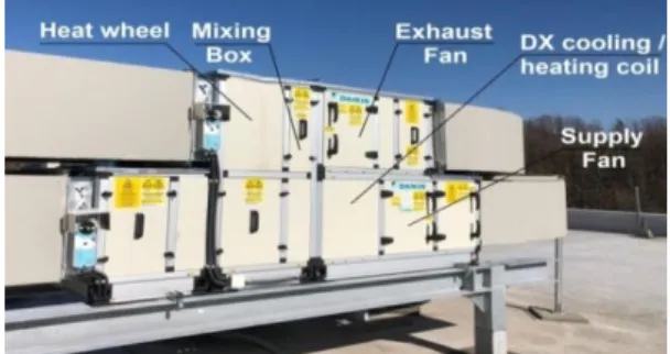
The main air handling components of the system are an air-to-air rotary heat wheel, a mixing box element, and direct expansion cooling/heating (DX) coil connected to a variable refrigerant volume outdoor unit. Figure1shows the elements of the investigated AHU.
Energies 2019, 12, x FOR PEER REVIEW 3 of 16
In this work, a field study is carried out on an existing, operating ventilation system that
94
includes an air-to-air rotary heat wheel, a mixing box element, and a direct expansion cooling coil
95
connected to a variable refrigerant volume outdoor unit. One of the main objectives of the present
96
paper is to investigate the cooling energy performance and thermal behavior of each air handling
97
component separately. To achieve this, an advanced data recording and remote monitoring system
98
was considerately developed by building management system-based software. The system includes
99
an electricity energy meter installed in the outdoor unit, as well as temperature, humidity, air
100
velocity, and CO2 sensors placed in the inlet and outlet section of all the air handling elements that
101
have an effect on the cooling process. The purpose of the CO2 measurements was to investigate the
102
CO2 cross-contamination, which occurs from the exhaust air flow to the supply air flow in the
103
air-to-air rotary heat wheel, resulting in indoor air quality degradation. The novelty of this research
104
is the accurate determination of the seasonal effectiveness and the energy saving impact of the heat
105
wheel on the electric energy consumption of the outdoor unit. Moreover, the relative average and
106
maximum value of CO2 cross-contamination in the rotary heat recovery using the developed
107
measurement system in the cooling period are presented. A further innovation in this study is the
108
analytical evaluation method developed, which shows a good agreement between the calculated
109
and measured energy consumption.
110
2. Materials and Methods
111
The selected air handling unit (AHU) is located on the flat roof of a shopping center, located in
112
the city of Eger in Hungary, which has supplied fresh air to the back-office and storage area of a
113
shop since 2017.
114
2.1. Description of the Investigated Central Ventilation System
115
The main air handling components of the system are an air-to-air rotary heat wheel, a mixing
116
box element, and direct expansion cooling/heating (DX) coil connected to a variable refrigerant
117
volume outdoor unit. Figure 1 shows the elements of the investigated AHU.
118
119
Figure 1. Photo from the investigated air handling units (AHU).
120
The specification of the AHU can be seen in Table 1.
121
Table 1. Specification of the investigated AHU [19].
122
Parameter Value Unit
Width × Height × Length 1450 × 1340 × 2897 mm
Air flow 1060 m3/h
External Pressure Drop 280 Pa
Weight 595 kg
Figure 2 shows the outdoor unit which is connected with refrigerant pipes to the DX coil and is
123
located in the AHU.
124 125
Figure 1.Photo from the investigated air handling units (AHU).
The specification of the AHU can be seen in Table1.
Table 1.Specification of the investigated AHU [19].
Parameter Value Unit
Width×Height×Length 1450×1340×2897 mm
Air flow 1060 m3/h
External Pressure Drop 280 Pa
Weight 595 kg
Figure2shows the outdoor unit which is connected with refrigerant pipes to the DX coil and is located in the AHU.
Energies2019,12, 4267 4 of 16
Energies 2019, 12, x FOR PEER REVIEW 4 of 16
126
Figure 2. Photo from the outdoor unit.
127
Technical data of the unit can be seen in Table 2.
128
Table 2. Technical data of the outdoor unit [19].
129
Parameter Value Unit
Total Cooling Capacity 10.9 kW
Refrigerant R410a -
EER 3.99 -
Fin Material Aluminium -
Tube Material Copper -
Table 3 shows the specification of the air-to-air recovery heat wheel in the cooling period.
130
Table 3. Specification of the investigated heat wheel [19].
131
Parameter Value Unit
Heat recovered 2 kW
Effectiveness 74.9 %
Diameter 600 mm
2.2. Description of the Developed Measurement System
132
In total, six temperature and relative humidity sensors, three CO2 sensors and three air velocity
133
sensors were placed in the inlet and outlet section of each air handling element and an electricity
134
energy meter was installed in the outdoor unit. The placement of the measurement points can be
135
seen in Figure 3. The technical data of the installed sensors and instrument can be read in Table 4.
136
137 138
Figure 3. Schematic diagram (a) for the placement of the measurement points on the real operating
139
AHU and (b) the AHU without a heat recovery operation assumption.
140
Figure 2.Photo from the outdoor unit.
Technical data of the unit can be seen in Table2.
Table 2.Technical data of the outdoor unit [19].
Parameter Value Unit
Total Cooling Capacity 10.9 kW
Refrigerant R410a -
EER 3.99 -
Fin Material Aluminium -
Tube Material Copper -
Table3shows the specification of the air-to-air recovery heat wheel in the cooling period.
Table 3.Specification of the investigated heat wheel [19].
Parameter Value Unit
Heat recovered 2 kW
Effectiveness 74.9 %
Diameter 600 mm
2.2. Description of the Developed Measurement System
In total, six temperature and relative humidity sensors, three CO2sensors and three air velocity sensors were placed in the inlet and outlet section of each air handling element and an electricity energy meter was installed in the outdoor unit. The placement of the measurement points can be seen in Figure3. The technical data of the installed sensors and instrument can be read in Table4.
Energies 2019, 12, x FOR PEER REVIEW 4 of 16
126
Figure 2. Photo from the outdoor unit.
127
Technical data of the unit can be seen in Table 2.
128
Table 2. Technical data of the outdoor unit [19].
129
Parameter Value Unit
Total Cooling Capacity 10.9 kW
Refrigerant R410a -
EER 3.99 -
Fin Material Aluminium -
Tube Material Copper -
Table 3 shows the specification of the air-to-air recovery heat wheel in the cooling period.
130
Table 3. Specification of the investigated heat wheel [19].
131
Parameter Value Unit
Heat recovered 2 kW
Effectiveness 74.9 %
Diameter 600 mm
2.2. Description of the Developed Measurement System
132
In total, six temperature and relative humidity sensors, three CO2 sensors and three air velocity
133
sensors were placed in the inlet and outlet section of each air handling element and an electricity
134
energy meter was installed in the outdoor unit. The placement of the measurement points can be
135
seen in Figure 3. The technical data of the installed sensors and instrument can be read in Table 4.
136
137 138
Figure 3. Schematic diagram (a) for the placement of the measurement points on the real operating
139
AHU and (b) the AHU without a heat recovery operation assumption.
140
Figure 3.Schematic diagram (a) for the placement of the measurement points on the real operating AHU and (b) the AHU without a heat recovery operation assumption.
Energies2019,12, 4267 5 of 16
Table 4.Specification of the sensors and instrument.
Model Device Working Range Accuracy
Honeywell VF20-3B65NW Temperature sensor −40–150◦C ±0.4◦C
Honeywell LFH20-2B65 Humidity sensor 10–90% ±3%
Honeywell AQS-KAM-20 CO2sensor 0–2000 ppm ±50 ppm
Honeywell AV-D-10 Air velocity sensor 2–20 m/s ±0.2 m/s
Inepro Metering Pro 380 Electricity energy meter 5–100 A ±1%
The recording of the measured data took place in an hourly period. With regards to the measurement accuracy, temperature sensors are normally used with a±0.4◦C accuracy, humidity sensors with a±3% accuracy, an air velocity sensor with a±0.2 m/s accuracy, carbon dioxide sensors with a±50 ppm accuracy, and an electric energy meter with a 1% of full scale accuracy. Among the monitoring air handling data, the air temperature and relative humidity data of the inlet and outlet sections of the DX cooling coil, energy recovery unit, and outdoor were used to investigate the energy performance and thermal behaviour of these air handling elements in the AHU in the cooling season.
The specification of the sensors and electricity energy meter used for monitoring of the investigated AHU can be seen in Table4.
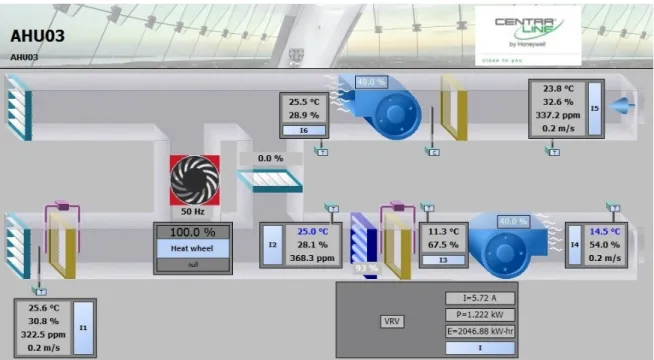
For the monitoring and recording of the various air condition parameters and the electrical energy consumption of the outdoor unit, the CentraLine Building Management System (BMS) software (version 2019) solution from Honeywell was implemented on a central server. Figure4shows a picture of the target building, along with a representative BMS screen for the investigated air handling unit.
Energies 2019, 12, x FOR PEER REVIEW 5 of 15
The recording of the measured data took place in an hourly period. With regards to the measurement accuracy, temperature sensors are normally used with a ±0.4 °C accuracy, humidity sensors with a ±3% accuracy, an air velocity sensor with a ±0.2 m/s accuracy, carbon dioxide sensors with a ±50 ppm accuracy, and an electric energy meter with a 1% of full scale accuracy. Among the monitoring air handling data, the air temperature and relative humidity data of the inlet and outlet sections of the DX cooling coil, energy recovery unit, and outdoor were used to investigate the energy performance and thermal behaviour of these air handling elements in the AHU in the cooling season.
The specification of the sensors and electricity energy meter used for monitoring of the investigated AHU can be seen in Table 4.
Table 4. Specification of the sensors and instrument.
Model Device Working range Accuracy Honeywell VF20-3B65NW Temperature sensor −40–150 °C ±0.4 °C
Honeywell LFH20-2B65 Humidity sensor 10–90% ±3%
Honeywell AQS-KAM-20 CO2 sensor 0–2000 ppm ±50 ppm Honeywell AV-D-10 Air velocity sensor 2–20 m/s ±0.2 m/s Inepro Metering Pro 380 Electricity energy meter 5–100 A ±1%
For the monitoring and recording of the various air condition parameters and the electrical energy consumption of the outdoor unit, the CentraLine Building Management System (BMS) software (version 2019) solution from Honeywell was implemented on a central server. Figure 4 shows a picture of the target building, along with a representative BMS screen for the investigated air handling unit.
Figure 4. A screenshot of the investigated AHU in the Building Management System (BMS).
Access to the BMS software was remotely enabled. Within this technical context, the necessary data were collected for this field study. Data were collected online at hourly intervals, saved, and stored on a computer from a distance.
3. Evaluation of the Data Recorded
To investigate the energy performance of the AHU, using the measurements, the following mathematical approaches were implemented.
Figure 4.A screenshot of the investigated AHU in the Building Management System (BMS).
Access to the BMS software was remotely enabled. Within this technical context, the necessary data were collected for this field study. Data were collected online at hourly intervals, saved, and stored on a computer from a distance.
3. Evaluation of the Data Recorded
To investigate the energy performance of the AHU, using the measurements, the following mathematical approaches were implemented.
Energies2019,12, 4267 6 of 16
3.1. Calculation Formulas for Measured Data Evaluation
Using the measured air temperature and relative humidity data, the specific humidity could be calculated to obtain the enthalpy of the air. To achieve this, the water vapor saturation pressure (Pws) was first calculated with Equation (1) [20]:
Pws=A·10(t+mttn)·100, (1) wherePws is the saturation pressure of the water vapor in Pa; t is the air temperature in◦C; and A, m, andtn are constant values in -. Since the temperature range during the measurements was between−20 and+50◦C, the constant values (in 0.083% maximum error) were as follows:A=6.116441;
m=7.591386;tn=240.7263 [20]. The constant value of 100 in Equation (1) represents the conversion of the saturation pressure of water vapor from hPa to Pa.
To obtain the moisture content, the partial pressure of water vapor in the air at a given relative humidity was also calculated with Equation (2) [20]:
Pw=Pws·RH
100, (2)
wherePwis the partial pressure of water vapor in Pa and RH is the relative humidity of the air in %.
The constant value of 100 in Equation (2) represents the conversion of relative humidity from % to -.
The moisture content was calculated with Equation (3) [21]:
x=0.622· Pw
Po−Pw, (3)
wherexis the moisture content of the air in kg/kg,Pois the barometric pressure in Pa, and the 0.622 constant value is the molecular weight ratio of water vapor to dry air.
The enthalpy was calculated with Equation (4) [21]:
h=cpa·t+x·(cpw·t+2500), (4) wherehis the enthalpy of the air in kJ/kg,cpais the specific heat of air at constant pressure in kJ/(kg·◦C), cpwis the specific heat of water vapor at constant pressure in kJ/(kg·◦C), and the constant value of 2500 represents the evaporation heat in kJ/(kg·◦C).
3.2. Formulas for Energy Calculations
Considering the fact that there is balanced ventilation, the effectiveness values of the heat wheel were determined from the air temperature measured values using Equation (5) [22,23]:
εs = (tHWS−to)
(tHWE−to), (5)
whereεSis the real sensible effectiveness of the heat wheel given by the measured data in -,tHWSis the air temperature in the supply outlet section of the heat wheel in◦C,tHWEis the air temperature in the exhaust inlet section of the heat wheel in◦C, andtois the ambient air temperature which is equal to the air temperature in the supply inlet section of the heat wheel in◦C.
To get information about the seasonal energy performance of the heat recovery during the cooling period, the average of the sensible effectiveness was calculated with Equation (6):
εs_AV= Pn
i=1εs_i
n , (6)
Energies2019,12, 4267 7 of 16
whereεs_AVis the average of the sensible effectiveness of the heat wheel given by the measured data in the cooling season in - and n is the number of measurements.
The maximum value of the sensible effectiveness was also analyzed during the whole cooling season, which was calculated with Equation (7):
εs_MAX=MAX(εs_i. . . εs_n), (7) whereεs_MAX is the maximum value of the sensible effectiveness of the heat wheel given by the measured data in the cooling season in -.
To calculate the energy saving of the heat wheel in the cooling season, Equation (8) was used:
QHW_saved=m.s·(ho−hHWS)·τ, (8) whereQHW_savedis the energy saving of the heat wheel in kWh;m.sis the air mass flow rate delivered by the fans in kg/s, which is calculated by the multiplication of the measured air velocity in m/s and the internal cross-section of air duct in 0.7398 m2and approached a 1.2 kg/m3constant air density; hois the ambient air enthalpy which is equal to the air enthalpy in the supply inlet section of the heat wheel in kJ/kg;hHWSis the air enthalpy in the supply outlet section of the heat wheel in kJ/kg; andτis the time in hours. The average air volume flow rate was evaluated as 1060 m3/h during the cooling season.
To calculate the cooling energy consumption of the DX coil, Equation (9) was used:
QDX_HW=m.s·(hHWS−hDX)·τ, (9) whereQDX_HWis the cooling energy consumption of the DX coil in kWh, and hDXis the air enthalpy in the supply outlet section of the DX coil in kJ/kg, which is equal to the supply air condition.
In order to investigate more the energy saving impact of the heat wheel on the DX coil, the cooling energy consumption of DX coil was also determined by Equation (10), neglecting the air-to-air rotary heat wheel operation, when the DX coil directly cools the hot ambient air to the supply air conditions.
QDX_WO_HW=m.s·(ho−hDX)·τ, (10) whereQDX_WO_HWis the cooling energy consumption of the DX coil without the heat wheel operation in kWh.
The calculated electric energy consumption of the outdoor unit was calculated with Equation (11):
PVRV_HW= QDX_HW
EER , (11)
wherePVRV_HWis the calculated electric energy consumption of the outdoor unit with the heat wheel operation in kWh, and EER is the energy efficiency ratio, given by the producer in -.
Moreover, the real electric energy consumption of the outdoor unit (PVRV_HW_M) was also measured during the cooling season, in order to see the agreement between values of the measured data and calculations using the recorded air condition parameters (PVRV_HW). The difference between the measured and calculated electric energy consumption was determined with Equation (12):
∆PVRV_HW=PVRV_HW_M−PVRV_HW, (12)
where∆PVRV_HWis the difference between the measured and calculated electric energy consumption of the outdoor unit with the heat wheel operation in kWh.
Energies2019,12, 4267 8 of 16
The rate of deviation of the measured and calculated electric energy consumption of the outdoor unit related to the measured data was calculated with Equation (13):
∆PVRV_HW_REL= ∆PVRV_HW PVRV_HW
·100, (13)
where∆PVRV_HW_RELis the rate of deviation of the measured and calculated electric energy consumption of the outdoor unit in %.
The electric energy consumption of the outdoor unit without the heat wheel operation was calculated with Equation (14):
PVRV_WO_HW= QDX_WO_HW
EER , (14)
wherePVRV_WO_HWis the electrical energy consumption of the outdoor unit without the heat wheel operation in kWh when it directly cools the hot ambient air to the supply air conditions via the DX coil during the cooling season.
The energy saving of the heat wheel in terms of the electric energy consumption of the outdoor unit was calculated with Equation (15):
∆PVRV_HW_saved=PVRV_WO_HW−PVRV_HW, (15) where∆PVRV_HW_saved is the amount of energy saved by the heat wheel in terms of the calculated electric energy consumption of the outdoor unit compared to that without the heat recovery operation in kWh.
The energy saving impact of the heat wheel on the electric energy consumption of the outdoor unit, compared to the system without the heat wheel operation, was calculated with Equation (16):
∆PVRV_HW_saved_REL= ∆PVRV_HW_saved
PVRV_WO_HW
·100, (16)
where∆PVRV_HW_saved_RELis the energy saving rate of the heat wheel for the electric energy consumption of the outdoor unit, compared to the system without heat the wheel operation, in %.
The value of the actual energy efficiency ratio of the outdoor unit given obtained the field study was determined with Equation (17) for the investigated cooling season to compare the data provided by the producer:
EERM= QDX_HW PVRV_HW_M
·100, (17)
whereEERMis the evaluated energy efficiency ratio (-) based on the measurement during the whole investigated cooling season.
3.3. Formulas for Carbon Dioxode Cross-Contamination in the Heat Wheel
The scale of carbon dioxide (CO2) cross-contamination in the air-to-air rotary heat recovery wheel was also investigated by measurements in the heat wheel during the operation of the air handling unit in the cooling period. To achieve this, the CO2concentration difference between the supply inlet and outlet sections of the heat wheel was first determined with Equation (18):
∆CCO2_cross=CCO2_HWS−CCO2_o, (18) where∆CCO2_crossis the scale of the CO2cross-contamination in the heat wheel in a given hour in ppm;
CCO2_HWSis the CO2concentration in the supply outlet section of the heat wheel in ppm; andCCO2_o
is the CO2concentration of the ambient air in ppm, which is equal to the CO2concentration in the supply inlet section of the heat wheel in ppm.
Energies2019,12, 4267 9 of 16
Having completed the measurements, the average of the CO2cross-contamination values was taken, and the ratio of the result and the supplied average CO2 concentration was calculated by Equation (19):
∆CCO2_cross_AV= Pn
i=1∆CCO2_cross_i
n , (19)
where∆CCO2_cross_AVis the average of the CO2cross-contamination values in ppm andnis the number of measurements.
Since CO2cross-contamination occurs from the exhaust section to the supply section in the heat wheel, the average of the measured CO2values in the exhaust inlet section of the heat wheel was also calculated with Equation (20) using the data measured:
CCO2_HWE_AV= Pn
i=1CCO2_HWE_i
n , (20)
whereCCO2_HWE_AVis the average value of the CO2concentration in the exhaust inlet section of the heat wheel in ppm andnis the number of measurements.
Equation (21) was used to obtain the relative average of differences:
∆CCO2_REL= ∆CCO2_cross_AV
CCO2_HWE_AV
·100, (21)
where ∆CCO2_REL is the relative average of CO2 cross-contamination in %, considering the CO2 concentration content in the exhaust inlet section of the heat wheel in ppm.
The maximum value of CO2cross-contamination was also analyzed during the whole cooling season, which was calculated with Equation (22):
CCO2_REL_MAX=
"
MAX CCO2_cross_i
CCO2_HWE_i. . . CCO2_cross_n
CCO2_HWE_n
!#
·100, (22)
whereCCO2_REL_MAXis the maximum value of CO2cross-contamination in the heat wheel in the cooling season given by the measured data in %.
4. Results and Discussion
The reference period of the study is the year 2019, more specifically, the cooling period from June 1st to August 31st for a total of 92 days and 25,296 data samples for each of the used measurement points. The AHU is intermittently operated 12 h/day from 8:00 till 20:00 7 days/week. Since this research work focused on the ventilation energy saving of the heat recovery unit’s DX cooling coil, the mixing box was shut offduring the data recording.
The air handling parameters obtained from the field study for the investigated AHU are illustrated in Figures5–7with a monthly timescale. Since the ambient air temperature was the highest in June during the whole cooling season, this relevant month was selected to present the measured data resulting from the data collection.
Figure5shows the temperature of the outdoor air (to), the air in the supply outlet sections of the heat wheel (tHWS) and DX coil (tDX), and the exhaust inlet section of the heat wheel (tHWE) over time at hourly intervals in June.
Considering the hottest periods in the cooling season, the ambient air temperature decreased by about 4–5◦C due to the pre-cooling effect of the heat wheel, and by an additional 18–20◦C, provided by air cooling of the DX coil.
Figure6shows the measured relative humidity of the outdoor air (RHo), the air in the supply outlet sections of the heat wheel (RHHWS) and DX coil (RHDX), and the exhaust inlet section of the heat wheel (RHHWE) over time at hourly intervals in June.
Energies2019,12, 4267 10 of 16
Energies 2019, 12, x FOR PEER REVIEW 9 of 16
where CCO2_REL_MAX is the maximum value of CO2 cross-contamination in the heat wheel in the cooling
274
season given by the measured data in %.
275
4. Results and Discussion
276
The reference period of the study is the year 2019, more specifically, the cooling period from
277
June 1st to August 31st for a total of 92 days and 25,296 data samples for each of the used
278
measurement points. The AHU is intermittently operated 12 h/day from 8:00 till 20:00 7 days/week.
279
Since this research work focused on the ventilation energy saving of the heat recovery unit’s DX
280
cooling coil, the mixing box was shut off during the data recording.
281
The air handling parameters obtained from the field study for the investigated AHU are
282
illustrated in Figures 5–7 with a monthly timescale. Since the ambient air temperature was the
283
highest in June during the whole cooling season, this relevant month was selected to present the
284
measured data resulting from the data collection.
285
Figure 5 shows the temperature of the outdoor air (to), the air in the supply outlet sections of the
286
heat wheel (tHWS) and DX coil (tDX), and the exhaust inlet section of the heat wheel (tHWE) over time at
287
hourly intervals in June.
288 289
290
Figure 5. The air temperature values in the air handling processes.
291
Considering the hottest periods in the cooling season, the ambient air temperature decreased by
292
about 4–5 °C due to the pre-cooling effect of the heat wheel, and by an additional 18–20 °C, provided
293
by air cooling of the DX coil.
294
Figure 6 shows the measured relative humidity of the outdoor air (RHo), the air in the supply
295
outlet sections of the heat wheel (RHHWS) and DX coil (RHDX), and the exhaust inlet section of the heat
296
wheel (RHHWE) over time at hourly intervals in June.
297
0 5 10 15 20 25 30 35 40
1-Jun-19 - 7 AM 1-Jun-19 - 6 PM 2-Jun-19 - 3 PM 3-Jun-19 - 1 PM 4-Jun-19 - 1 AM 5-Jun-19 - 7 AM 5-Jun-19 - 6 PM 6-Jun-19 - 3 PM 7-Jun-19 - 12 PM 8-Jun-19 - 9 AM 8-Jun-19 - 8 PM 9-Jun-19 - 5 PM 10-Jun-19 - 3 PM 11-Jun-19 - 12 PM 12-Jun-19 - 9 AM 12-Jun-19 - 8 PM 13-Jun-19 - 5 PM 14-Jun-19 - 2 PM 15-Jun-19 - 11 AM 16-Jun-19 - 8 AM 16-Jun-19 - 7 PM 17-Jun-19 - 5 PM 18-Jun-19 - 2 PM 19-Jun-19 - 11 AM 20-Jun-19 - 8 AM 20-Jun-19 - 7 PM 21-Jun-19 - 4 PM 22-Jun-19 - 1 PM 23-Jun-19 - 10 AM 24-Jun-19 - 8 AM 24-Jun-19 - 7 PM 25-Jun-19 - 4 PM 26-Jun-19 - 1 PM 27-Jun-19 - 10 AM 28-Jun-19 - 7 AM 28-Jun-19 - 6 PM 29-Jun-19 - 3 PM 30-Jun-19 - 12 PM
t [°C]
t_o t_HWS t_DX t_HWE
[h]
Figure 5.The air temperature values in the air handling processes.
Energies 2019, 12, x FOR PEER REVIEW 10 of 16
298
Figure 6. The air relative humidity values in the air handling processes.
299
The ambient air relative humidity decreased by about 60% due to the air cooling process. In this
300
way, the supplied air relative humidity was around 90%.
301
Figure 7 shows the enthalpy of the outdoor air (ho), the air in the supply outlet sections of the
302
heat wheel (hHWS) and DX coil (hDX), and the exhaust inlet section of the heat wheel (hHWE) over time
303
at hourly intervals in June.
304
305
Figure 7. The air enthalpy values in the air handling processes.
306
Considering the hottest periods in the cooling season, the ambient air enthalpy decreased by
307
about 8–10 kJ/kg due to the pre-cooling effect of the heat wheel, and by an additional 30–35 kJ/kg,
308
provided by air cooling of the DX coil.
309
Figure 8 shows the sensible effectiveness data (s) for the outdoor air temperature in June.
310
0 10 20 30 40 50 60 70 80 90 100
1-Jun-19 - 7 AM 1-Jun-19 - 6 PM 2-Jun-19 - 3 PM 3-Jun-19 - 1 PM 4-Jun-19 - 1 AM 5-Jun-19 - 7 AM 5-Jun-19 - 6 PM 6-Jun-19 - 3 PM 7-Jun-19 - 12 PM 8-Jun-19 - 9 AM 8-Jun-19 - 8 PM 9-Jun-19 - 5 PM 10-Jun-19 - 3 PM 11-Jun-19 - 12 PM 12-Jun-19 - 9 AM 12-Jun-19 - 8 PM 13-Jun-19 - 5 PM 14-Jun-19 - 2 PM 15-Jun-19 - 11 AM 16-Jun-19 - 8 AM 16-Jun-19 - 7 PM 17-Jun-19 - 5 PM 18-Jun-19 - 2 PM 19-Jun-19 - 11 AM 20-Jun-19 - 8 AM 20-Jun-19 - 7 PM 21-Jun-19 - 4 PM 22-Jun-19 - 1 PM 23-Jun-19 - 10 AM 24-Jun-19 - 8 AM 24-Jun-19 - 7 PM 25-Jun-19 - 4 PM 26-Jun-19 - 1 PM 27-Jun-19 - 10 AM 28-Jun-19 - 7 AM 28-Jun-19 - 6 PM 29-Jun-19 - 3 PM 30-Jun-19 - 12 PM
RH[%]
RH_o RH_HWS RH_DX RH_HWE
[h]
20 30 40 50 60 70 80 90
1-Jun-19 - 7 AM 1-Jun-19 - 8 PM 2-Jun-19 - 7 PM 3-Jun-19 - 7 PM 4-Jun-19 - 6 PM 5-Jun-19 - 5 PM 6-Jun-19 - 4 PM 7-Jun-19 - 3 PM 8-Jun-19 - 2 PM 9-Jun-19 - 1 PM 10-Jun-19 - 1 PM 11-Jun-19 - 12 PM 12-Jun-19 - 11 AM 13-Jun-19 - 10 AM 14-Jun-19 - 9 AM 15-Jun-19 - 8 AM 16-Jun-19 - 7 AM 17-Jun-19 - 7 AM 17-Jun-19 - 8 PM 18-Jun-19 - 7 PM 19-Jun-19 - 6 PM 20-Jun-19 - 5 PM 21-Jun-19 - 4 PM 22-Jun-19 - 3 PM 23-Jun-19 - 2 PM 24-Jun-19 - 2 PM 25-Jun-19 - 1 PM 26-Jun-19 - 12 PM 27-Jun-19 - 11 AM 28-Jun-19 - 10 AM 29-Jun-19 - 9 AM 30-Jun-19 - 8 AM
h[kJ/kg]
h_o h_HWS h_HWE h_DX
[h]
Figure 6.The air relative humidity values in the air handling processes.
The ambient air relative humidity decreased by about 60% due to the air cooling process. In this way, the supplied air relative humidity was around 90%.
Figure7shows the enthalpy of the outdoor air (ho), the air in the supply outlet sections of the heat wheel (hHWS) and DX coil (hDX), and the exhaust inlet section of the heat wheel (hHWE) over time at hourly intervals in June.
Considering the hottest periods in the cooling season, the ambient air enthalpy decreased by about 8–10 kJ/kg due to the pre-cooling effect of the heat wheel, and by an additional 30–35 kJ/kg, provided by air cooling of the DX coil.
Energies2019,12, 4267 11 of 16
Energies 2019, 12, x FOR PEER REVIEW 10 of 15
Figure 6. The air relative humidity values in the air handling processes.
The ambient air relative humidity decreased by about 60% due to the air cooling process. In this way, the supplied air relative humidity was around 90%.
Figure 7 shows the enthalpy of the outdoor air (ho), the air in the supply outlet sections of the heat wheel (hHWS) and DX coil (hDX), and the exhaust inlet section of the heat wheel (hHWE) over time at hourly intervals in June.
Figure 7. The air enthalpy values in the air handling processes.
Considering the hottest periods in the cooling season, the ambient air enthalpy decreased by about 8–10 kJ/kg due to the pre-cooling effect of the heat wheel, and by an additional 30–35 kJ/kg, provided by air cooling of the DX coil.
Figure 8 shows the sensible effectiveness data (εs) for the outdoor air temperature in June.
0 10 20 30 40 50 60 70 80 90 100
1-Jun-19 - 7 AM 1-Jun-19 - 6 PM 2-Jun-19 - 3 PM 3-Jun-19 - 1 PM 4-Jun-19 - 1 AM 5-Jun-19 - 7 AM 5-Jun-19 - 6 PM 6-Jun-19 - 3 PM 7-Jun-19 - 12 PM 8-Jun-19 - 9 AM 8-Jun-19 - 8 PM 9-Jun-19 - 5 PM 10-Jun-19 - 3 PM 11-Jun-19 - 12 PM 12-Jun-19 - 9 AM 12-Jun-19 - 8 PM 13-Jun-19 - 5 PM 14-Jun-19 - 2 PM 15-Jun-19 - 11 AM 16-Jun-19 - 8 AM 16-Jun-19 - 7 PM 17-Jun-19 - 5 PM 18-Jun-19 - 2 PM 19-Jun-19 - 11 AM 20-Jun-19 - 8 AM 20-Jun-19 - 7 PM 21-Jun-19 - 4 PM 22-Jun-19 - 1 PM 23-Jun-19 - 10 AM 24-Jun-19 - 8 AM 24-Jun-19 - 7 PM 25-Jun-19 - 4 PM 26-Jun-19 - 1 PM 27-Jun-19 - 10 AM 28-Jun-19 - 7 AM 28-Jun-19 - 6 PM 29-Jun-19 - 3 PM 30-Jun-19 - 12 PM
RH[%]
RH_o RH_HWS RH_DX RH_HWE
τ[h]
20 30 40 50 60 70 80 90
1-Jun-19 - 7 AM 1-Jun-19 - 8 PM 2-Jun-19 - 7 PM 3-Jun-19 - 7 PM 4-Jun-19 - 6 PM 5-Jun-19 - 5 PM 6-Jun-19 - 4 PM 7-Jun-19 - 3 PM 8-Jun-19 - 2 PM 9-Jun-19 - 1 PM 10-Jun-19 - 1 PM 11-Jun-19 - 12 PM 12-Jun-19 - 11 AM 13-Jun-19 - 10 AM 14-Jun-19 - 9 AM 15-Jun-19 - 8 AM 16-Jun-19 - 7 AM 17-Jun-19 - 7 AM 17-Jun-19 - 8 PM 18-Jun-19 - 7 PM 19-Jun-19 - 6 PM 20-Jun-19 - 5 PM 21-Jun-19 - 4 PM 22-Jun-19 - 3 PM 23-Jun-19 - 2 PM 24-Jun-19 - 2 PM 25-Jun-19 - 1 PM 26-Jun-19 - 12 PM 27-Jun-19 - 11 AM 28-Jun-19 - 10 AM 29-Jun-19 - 9 AM 30-Jun-19 - 8 AM
h[kJ/kg]
h_o h_HWS h_HWE h_DX
τ[h]
Figure 7.The air enthalpy values in the air handling processes.
Figure8shows the sensible effectiveness data (εs) for the outdoor air temperature in June.
Energies 2019, 12, x FOR PEER REVIEW 11 of 16
311
Figure 8. The sensible effectiveness values as a function of outdoor air temperature in June.
312
Based on the results, the average sensible effectiveness of the heat wheel was 79.6% during the
313
whole cooling season and the maximum value of 97.6% was recorded in June.
314
Figure 9 shows the energy saving of the air-to-air rotary heat wheel (QHW_saved) in terms of the
315
energy consumption of the DX coil, and the cooling energy consumption of the DX coil with the heat
316
wheel operation (QDX_HW) and without the heat wheel operation (QDX_WO_HW), when the DX coil
317
directly cools the hot ambient outdoor air to the supply air conditions during the cooling season.
318 319
320
Figure 9. The energy recovery and auxiliary cooling energy consumption for ventilation.
321
Based on the results, the energy saving of the heat wheel was 2491 kWh in terms of the energy
322
consumption of the DX coil, the cooling energy consumption of the DX coil with the heat wheel
323
operation was 7434 kWh, and that without the heat wheel operation was 9926 kWh.
324
Figure 10 shows the electric energy consumption of the outdoor unit based on the direct real
325
electric energy consumption measurements (PVRV_HW_M) and the calculations made using the
326
recorded air condition parameters with (PVRV_HW) and without the heat wheel operation (PVRV_WO_HW)
327
for the whole cooling period.
328
0 10 20 30 40 50 60 70 80 90 100
25,0 26,2 27,0 27,7 28,0 28,2 28,6 28,9 29,3 29,5 29,9 30,1 30,5 30,6 30,9 31,3 32,0 32,2 32,4 32,6 33,0 33,1 33,4 33,6 34,0 34,5 34,8 35,6 36,0
s [%]to[°C]
2491
7434
9926
0 2000 4000 6000 8000 10000 12000
1 2 3
QHW_saved QDX_HW QDX_WO_HW
Figure 8.The sensible effectiveness values as a function of outdoor air temperature in June.
Based on the results, the average sensible effectiveness of the heat wheel was 79.6% during the whole cooling season and the maximum value of 97.6% was recorded in June.
Figure9shows the energy saving of the air-to-air rotary heat wheel (QHW_saved) in terms of the energy consumption of the DX coil, and the cooling energy consumption of the DX coil with the heat wheel operation (QDX_HW) and without the heat wheel operation (QDX_WO_HW), when the DX coil directly cools the hot ambient outdoor air to the supply air conditions during the cooling season.