Model-based Power Generation Estimation of Solar Panels using Weather Forecast for
Microgrid Application
Roland Bálint, Attila Fodor and Attila Magyar
University of Pannonia, Faculty of Information Technology, Egyetem u. 10, H-8200 Veszprém, Hungary
E-mails: balint.roland@virt.uni-pannon.hu, foa@almos.uni-pannon.hu, magyar.attila@virt.uni-pannon.hu
Abstract: An electrical power production estimation model has been proposed in this paper for PV panels. The model uses weather forecast data of a time interval (e.q. one day ahead) as input and gives an estimation to electricity generation for the same time interval. The proposed method takes into account the thermal effects taking place in a solar panel as well as the temperature dependent nature of the solar panel efficiency. The results of this paper could be utilized by transmission system operator, distribution system operator, virtual power plant and microgrid operators. The precise mathematical model of the renewable energy resources, which the function of the weather forecast is necessary for the very large scale integration to the electrical transmission system.
Keywords: PV power plant; Power estimation; modeling; thermal dependence; distributed energy resources
1 Introduction
Solar radiation models have been used for the prediction of the amount of energy available by solar irradiance. The primary application area of such models were ecological studies. The irradiance model proposed in [1] determines the amount of solar irradiance for given areas in a monthly and daily manner for climatic studies.
Nowadays, the primary field of application of irradiance models is photovoltaic generation using solar power plants. As the number of such appliances constantly grows the importance of any solution that improves the stability, power quality, optimality of the distribution network using photovoltaic units is increasing as well.
Unfortunately, solar generation (and wind generation as well) lacks the advantageous properties of predictability and controllability, which is available for fossil and nuclear power plants. The electrical power generated by PV panels can only be optimized by geometric parameters of the installation and the design of an appropriate solar tracking system [2]. The electrical power generated by renewable generators highly depends on actual weather, i.e. the amount of power generated is constantly fluctuating. As the proportion of renewables in the total electrical energy increases this unpredictably fluctuating generation causes several power network safety related issues [3].
In some countries to counterweight the uncertainty represented by the renewable generation, the operators of non home size photovoltaic power plant are obligated to present a power generation plan. The distribution system operator specifies the rules for amount of curtailment and possible compensation (penalty), that case there is difference between the planned and the actual generation. From the PV power plant (PVPP) operator point of view the minimization of this penalty is vital, and any solution for the prediction of the generation is welcome.
The power production timing is one of the most important tasks of the transmission system operator (TSO), distribution system operator (DSO), virtual power plant (VPP) and microgrid operators. The opertator has to estimate the customer loads and the power generation from renewable energy sources (RES).
There are different operation and management strategies for the operators of the distribution network, the transmission network, the power generators or the microgrid [4], [5]. It is crucial for the microgrid operation algorithm to have an approximate information about the electrical power generated from the renewable sources (solar or wind) so that the changes can be compensated (e.q. by charging/discharging a battery, enable/disable loads, turning diesel generator on/off, etc.) [6].
On the other hand, power network security regards are just as important as the previously mentioned financial viewpoints. There are several network stability and energy quality related indicators, among them energy balance is crucial for the operation safety point of view. In order to ensure the energy balance of the power network, the classical power plants are controlled in order that the total generation meets the demand despite of the uncertainty of the renewable generators present on the network. The successful energy balancing depends on two main factors, the available energy generation reserve that can be prescribed to the power plants, and an appropriate demand and renewable generation forecast. Moreover, for the operation and control of energy-positive systems the estimation and/or prediction of power is a key issue [7], [8].
The solar energy comes to the Earth in the form of radiation from the Sun.
Therefore, every solar power prediction model, is based on some solar geometry model. These models differ mainly in the level of detailedness, e.g. [9] presents a geometry model taking the different wavelength into account. On the other hand,
e.g. [10], [11] gives a more simple model. The first class of photovoltaic models deal with the PV panel characteristics [12], [13], in the work [14] the PV model parameters are estimated from long-term outdoor measurements. Others involve cooling effect (either air cooling of hybrid panel), e.g. the paper [15] examines the effect of cooling medium and the cooling system on the panel parameters. Hybrid panels are investigated in [16], where the efficiency of the panel is increased by a model based technique [17]. In the modeling of hybrid PV panels the temperature of the water is a key variable, which is estimated in [18].
The temperature dependent modeling of PV panels is important because the efficiency decreases with the temperature rising [19]. Work [20] proposed a thermal model of a PV panel that takes the infrared domain into account, others, e.g. [21] propose a simplified thermal model. Different geometrical parameters (e.g. inclination and orientation) might have effect on the thermal behavior [22].
Data-driven methods are very popular in every field of engineering [23], [24], the same holds for predictive solar generation models [25], [26], [27], [28]. In Ref.
[29] an adaptive predictive model is proposed that adapts the model parameters to the actual measurements; however, it uses only clear sky data, i.e. does not take the clouds into account. Artificial intelligence based prediction is a popular subclass, e.g. [3] proposes a short-term (1-2 hours) prediction where an AI based forecast method learns from the measurements and the actual cloud level. The authors of Ref. [30] propose a short-term irradiance forecast model that uses the results of several models.
The proposed predictive photovoltaic power generation model uses standard weather forecast data as input and predicts the generated power by taking the thermal efficiency decreasion of the panel into account. The model is based on a previously developed solar geometry model [31].
2 Modeling and Estimation of Solar Power Generation
The power generation estimation of PV power plants involves three functional modules:
estimation of the global solar irradiation of the PV panel slope,
estimation of the PV panel temperature for actual modul efficiency,
weather forecast data for PV plant localization.
The following sections describe the above modules of the proposed estimation method.
2.1 Estimation Model of Power Generation
In the previous work [31] a simple model has been described for calculating the global horizontal solar irradiance using astronomical relationships (equations (1)-(3)). From this data the global solar irradiance has been calculated on a surface for a given orientation (azimuth and tilt angle) (4). The solar irradiance on the PV panels can be calculated from the irradiance on the horizontal surface using the geometrical parameters of the installation of the PV panels [31].
d
m
d b
d z
T B d n
hor
I A e a N
G sin( )
1
(1)
d
mz b
T d n
hor
I A q N
S sin( )
1
(2)hor hor
hor
G S
D
(3)2 ) ) cos(
1 )
sin(
)
sin(
pvhor pv
hor
pv
S D
G
(4)The pvis the solar beam altitude angle on the PV surface. The power production of a PV power plant is given as the parametric model defined by equation (5).
) ( )
, ,
(
pv pv pv pv pvpv
pv
G N A T
P
, (5)where Gpv is the global solar irradiance on the modul surface as a function of cloudiness (N) and orientation (pv azimuth and pv tilt angle), the total surface Apv of the PV power plant and the PV moduls actual efficiency is pv which depends on the module temperature Tpv.
As opposed to the previous model [31] this model takes the clouds and the panel efficiency into account. The PV panels nominal efficiency (irradiance of 1000 W m2 and 25 °C cell temperature) and the temperature coefficients are obtained from the PV panel datasheet. The actual model efficiency is determined from the module temperature, which is also a variable of the proposed model. The level of cloudiness is represented by a value between 0 and 1 defined by formula (6).
threshold cloud
if
threshold cloud
if cloud
N f
C, 1
), (
(6)
If the cloud value (type of cloudiness) reaches a threshold value, then the N is constant 1. Below the threshold the N is a function of the type of cloudiness. In case of cloudless sky the N value is zero.
5 . 0 cos
5 . 0
:
theshold
cloud
f
C
(7)
2.2 PV Modul Temperature Estimation Model
As it was stated before in Section 2.1 PV panel efficiency depends on the panel temperature Tpv, i.e. the proposed model has to have a thermal module that estimates panel temperature. Panel temperature is influenced by solar irradiance on the PV panel (Gpv), the temperature of the environment (Tair) and of the panel (Tpv), the heat transfer coefficient (air) between panel and air (depends on the wind) and the efficiency (pv) according to formula (8) below.
) , , , ,
(
pv air pv air pvT
pv
f G T T
T
(8)This thermodynamic effect can be described by the ordinary differential equation (ODE) (9), where Cpvis the heat capacity and mpv is the mass of the PV modul. A multiplier of 2 is appearing next to the surface Apv since both the top and bottom sides of the panel are taken into account in the heat conduction.
pv pv pv
pv pv
pv pv air
pv air
pv
G
m c m c T A
T
T
2 1
)
(
(9)The overall value of the expression
c
pv m
pv in (9) can be expressed in more details based on the elementary building materials of the PV panel (formula (10)).plastic plastic
Si Si Al Al glass glass pv
pv
m c m c m c m c m
c
(10)The inhomogeneous ordinary differential equation (9) can be expressed in state space representation using the state and input vector defined in formula (11).
pv air
pv
G
T u T
x ,
(11)Afterwards, the state space model of the thermal module is given by formula (12) below.
pv air pv pv
pv pv
pv pv air
pv pv pv
pv air
pv
G
T m c m c T A
m c
T A
2 2 1
(12)It is important to note, that although a linear time invariant (LTI) state space model is used here, the model is nonlinear, since pv is a linear function of the panel temperature (with the slope of 0.4%C).
Since the estimator is implented in a discrete time manner, the thermal model (12) has to be discretized. In order to do that the parametric values of the state (A) and input matrix (B) are needed (13).
pv pv
pv pv
pv pv air
pv pv
pv
air
c m c m
A m
c
A
2 , 2 1
B
A
(13)The equistant sampling (TS 15min) of the state equation (12) gives a discrete time state equation which is a different equation of the form (14)
k T
s x k T
s u k T
s
x 1 Φ Γ
, (14)where the discrete time state (Φ) and input (Γ) matrices are obtained using the formula (15).
I B
Γ A
Φ e
ATs,
1 e
ATs
(15)The parametric state matrix is given below in equation (16), where TS is the sample time in seconds.
pv pv s
pv air s
T m c
A
T
e
e
2
Φ
A (16)The discterized input matrix can be calculated using (16). The input matrix of the disctere time model is given parametrically in equation (17) below.
s pv pv
pv air s
pv pv
pv air s
m T c
A
pv air
pv m T
c A T
A e e
e
2 2
1
2 1 1 1
B
I
Γ A
A(17)
Note, that Γ and Φ depend on the wind through air and the panel temperature through pv. However, this functional relationship has a constrained derivative, and it is regarded to change slowly with time (through panel temperature). This is why the above matrix Φ and Γhave to be calculated in each sampling interval.
2.3 Weather Forecast Data
The reliable weather forecast is important for the correct operation of the proposed model. Unfortunately, different weather forecast providers use different time resolution, level of detail, data included, moreover, they are using different models to calculate the forecast. The power prediction model uses the weather forecast variables (Tair,N, wind) for the next 24 hours (15 minutes step), but the weather forecasts usually give data of 1 or 3 hours time step.
For validation purposes, several different meteorological models and weather forecast providers are used for the same geographical location (where the PV panels are located). In the present work, the following six different weather forecast are used obtained from [32]:
Global Forecast System model (GFS) [33]: 3 days forecast, 3 hours resolution
Icosahedral Nonhydrostatic model (ICON) [34]: 3 days forecast, 1 hour resolution
Action de Recherche Petite Echelle Grande Echelle model (ARPEGE) [35]: 3 days forecast, 1 hour resolution
Global Environmental Multiscale model (GEM) [36] [37]: 3 days forecast, 3 hours resolution
High Resolution Limited Area Model (HIRLAM) Finland (FMI) [38]
[39]: 2 days forecast, 1 hour resolution
High Resolution Limited Area Model (HIRLAM) Netherlands (KNMI) [38] [39]: 2 days forecast, 1 hour resolution
The data structure of the weather forecast contains the following weather variables:
date [yyyy-mm-dd HH:MM]
temperature [°C]
wind speed [m/s]
cloud ϵ {0, 1, 2, 3, 4, 5, 6}
o 0: cloudless o 1: few clouds o 2: moderate clouds o 3: cloudy
o 4: full cloudy with little rain o 5: full cloudy with rain
o 6: full cloudy with thunderstorm
As the power production model uses a 15 minute sample time, the above forecasts need to be interpolated with third order splines.
Figure 1
Weather forecast temperature (Tair) and wind of the different models together with the real (measured) weather data in a three day interval
Figure 1 shows a three day sample of the different weather forecast together with the measured weather data (Tair and wind) It is apparent on the top of Figure 1, that the temperature forecasts are reliable since the main dynamics changes in the measured data which appears in all the forecasts.
The wind forecast (bottom of Figure 1) have a higher level of error since the wind gusts, the quick changes are not predictable and the terrain objects also affect wind speed. 5m s difference between the forecast and the real wind speed causes only 2 or 3 °C error in PV modul temperature. This error only results in a 1-2%
deviation in the estimation of power production.
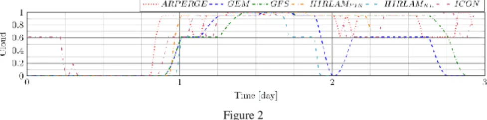
Figure 2 summarizes the different cloud forecasts of the weather models. The plots show the values of the functional relationship (6) based on the different cloud forecasts. As the lower level of clouds would result in faulty irradiance data due to the locally appearing clouds, these forecasts are not verified using measurements.
Figure 2
Cloud forecast for a 3 day horizon
It is important to note, that the cloud has the main effect on the PV power generation. Therefore, it is worthwhile to look at the performance of the models in terms of cloud forecast.
3 Verification and Validation of the Model
As a first step, the model proposed in Section 2 needs to be verified against engineering expectations. In order to do that, measured weather data has been used instead of forecast, and the model output has been examined against the actually measured power generation data. The proposed thermal model and the power generation estimation model are investigated in Sections 3.1 and 3.2, respectively. Section 3.3 proposes the validation results of the model using weather forecast data.
For both verification and validation the measured data and the parameters of installation (angles, surface size, efficiency) of a real system has been used. As the aim is to keep the model as simple as it is possible the territorial specialties (shadows of panels, trees, buildings) have been neglected.
3.1 Verification of the PV Panel Temperature Estimation Submodel
The PV panel temperature estimation submodel has been tested using measured input variables (global irradiance, wind, environment temperature) and the results (estimated PV module temperature) has been compared with to the actually measured module temperature. The results of the experiments are depicted in Figure 3 and Figure 4.
Figure 3
PV panel temperature estimation results on cloudy days
It is apparent in both figures that there is a difference between measured air and panel temperatures during the night hours although, due to expectations the panel
temperature should converge to air temperature. This difference comes from the calibration error of the module temperature measurement system and the fact, that panel temperature and air temperature measurements were performed at different points of the facility.
Figure 4
PV panel temperature estimation results on partially cloudy days
The error between the estimated and measured module temperature is more noticeable in Figure 4, however, the key dynamics are reproduced by the thermal submodel of the proposed estimator.
As a result of the verification it can be stated that the PV module temperature estimation model is acceptable for our purposes and it can serve as one of the components of the proposed PV production estimator model. Note that the role of temperature is important in panel efficiency (pv).
3.2 Verification the Photovoltaic Power Generation Estimator Submodel
In what follows, the whole solar power generation model is verified in the similar way as the thermal module was tested in Section 3.1. Note, that this time the estimated panel temperature is used for estimating the thermal efficiency pv. All the input variables of the model (environment temperature, wind speed and global solar irradiance) are obtained from historical measurements. The calculated power generation estimate is compared to the measured power generation for the same time interval.
A sample plot is presented in Figure 5 where the power generation of three consecutive days with different levels of cloudiness can be seen (sunny, fully cloudy, partially cloudy, respectively).
The power production model of PV plant with measured data input performs well and using appropriate weather forecasting the power production can be estimated for the next days.
Figure 5
Powered energy estimation of the PV model with using measured temperature, wind and global irradiance data
3.3 Validation of the Estimation Model using Weather Forecast Data
As a next step in the analysis of the proposed estimator, it has been validated using different weather forecasts as inputs and the model output (electrical energy generation) has been compared to the actual measured power generation for a five day interval with several different weather conditions.
Energy suppliers and network operators use a 15 minute time step for data acquisition and control/scheduling. Therefore, selection of 15 minute as a sampling time for the model is natural. On the other hand, weather forecasts generally use a larger sampling time (1-3 hours) this complication is resolved by interpolating (linear or spline) the weather forecast data at the intermediate time instances.
The results of the validation experiments and measurements are collected in Figure 6, where the predicted power generation together with the measured data are ploted for two days with different weather conditions.
The left plot of Figure 6 shows the results for a sunny day, where the solid line corresponds to the measured solar power generation while the dotted and dashed lines denote the predicted power production based on two of the weather forecast models (ARPEGE and HIRLAM_FIN, respectively). The dashdotted and the dashdotdotted lines show the cloudiness predicted by the corresponding weather models.
The right plot of Figure 6 is more interesting since it belongs to a cloudy day. The fluctuation in the measured power generation (oscillations on the solid line) caused by the shadowing clouds passing by over the solar panel. Each such event starts with a drop in the generation because of the decreased irradiation.
Figure 6
Measured and estimated energy production and cloud of two models on a sunny (left) and a cloudy (right) day
As the lack of sunshine cools down the panels, their efficiency pv increases which results in a jump in the power generation when the shadows leave the panel.
These transients do not appear in the power prediction curves as weather forecasts are not able to give such a precicse information about clouds.
Table 1 summarizes the results of the 5 day experiment using the input data of six different weather forecasts. Note, that each days power generation was predicted from a one day ahead either forecast. The data appearing in the cells are the prediction errors (both in Wh and relative error) of the proposed model using the corresponding weather forecast model as input. It is important to note, that the precision of the power generation prediction correlates with the precision of the weather forecast, i.e. the goodness of the proposed power production is determined by the goodness of the used weather forecast model.
The first two days of the examined 5 day interval were cloudless days with sunshine while the last three days were fully and partially cloudy days. In the first and second columns of Table 1 it can be seen that most of the models predicted the weather (and consequently, the power generation) well except ARPEGE and ICON (a few clouds were promised by these two forecast providers for this day).
The most interesting is the last three columns of the cloudy days, where the weather forecast models separate well.
The average and the average absolute deviations of each forecast model are given in the last two columns of Table 1.
It can be seen that by the end of the examined interval, the solar power generation model based on the ARPEGE weather forecast performed the best, followed by the HIRLAM_FIN based predictor.
Table 1
The difference values between the measured and estimated power generation based on the 6 different weather forecast models (first column) and 5 continuous day forecasted data series in Wh and % (100%
is the measured production). The last two columns are the average of the 5 days difference and the average of the absolute values.
Day 1
sunny
Day 2 sunny
Day 3 fully cludy
Day 4 part cloudy
Day 5
part cloudy AVG AVG (abs) ARPEGE [35] -5737,4 Wh 1027,3 Wh -963,8 Wh 2935,9 Wh 1220,6 Wh -303,5 Wh 2377,0 Wh
-12,27% 2,15% -16,94% 14,17% 3,31% -1,92% 9,77%
GEM [36]
[37]
656,8 Wh 878,2 Wh 4114,4 Wh 14930,0 Wh -8938,7 Wh 2328,1 Wh 5903,6 Wh
1,40% 1,83% 72,31% 72,05% -24,26% 24,67% 34,37%
GFS [33] 1931,9 Wh 711,9 Wh -3501,0 Wh -13813,0 Wh -22365,0 Wh -7407,0 Wh 8464,6 Wh
4,13% 1,49% -61,53% -66,60% -60,69% -36,64% 38,89%
HIRLAM_FIN [38] [39]
1606,2 Wh 880,9 Wh -1031,4 Wh -10432,0 Wh -4165,5 Wh -2628,4 Wh 3623,2 Wh
3,43% 1,84% -18,13% -50,35% -11,30% -14,90% 17,01%
HIRLAM_NL [38] [39]
-2248,6 Wh 1082,0 Wh -4117,4 Wh 11222,0 Wh -2117,6 Wh 764,1 Wh 4157,5 Wh
-4,81% 2,26% -72,36% 54,16% -5,75% -5,30% 27,87%
ICON [34] -28650,0 Wh 579,3 Wh 1195,5 Wh -13910,0 Wh -6746,9 Wh -9506,4 Wh 10216,3 Wh
-61,27% 1,21% 21,01% -67,13% -18,31% -24,90% 33,79%
3.4 Discussion of the Results
To summarize the simulation and experimental results of the verification and validation analysis Sections 3.1-3.3 it can be stated that the model proposed in Section 2 is viable.
The verification experiments (Figure 3, Figure 4 and Figure 5) confirmed that the solar power generation model together with the thermal submodel performs well and using actual measured weather data instead of forecasts, the proposed model reliably produced the results almost identical with the measured values (panel temperature, and produced energy).
The weather forecast based validation experiment showed that the key question is in the selection of the weather forecast. As for the experiments performed, ARPEGE [32] model supplemented out model the best however, the goodness of the weather forecast depends on several factors.
Although this five day experiment is far from being enough in the statistical sense, but it is enough to see that the proposed model based solar power generation prediction framework is a viable approach.
Conclusions
A model based approach has been presented in this paper that is able to estimate the energy production of solar panels based on an appropriate weather forecast. It is important to note that the preciseness of the proposed method is determined by the preciseness of the applied weather forecast model. The selection of the best
weather forecast model for a certain geographical location or classifying the forecast models based on the weather events is not out of the scope of this paper.
The model can also be used with a short-term (few hours ahead) and more precise weather forecast in order to improve the short-term energy balance and to avoid possible system failures (e.q. energy loss because of a cloud drift).
The furher research directions include the improve the weather forecast precision by contacting the local meteorological service to provide a geologically more focused foracast. Another improvement that will be made is to not only take into account the extension but also the type of clouds (i.e. density, height). The model can also be used for sizing energy storage capacities fo fill the gaps between energy peaks and valleys caused by clouds.
Acknowledgement
This research is partially supported by the National Research, Development and Innovation Office - NKFIH through grant No. 120422. We acknowledge the financial support of Széchenyi 2020 under the GINOP-2.2.1-15-2017-00038.
References
[1] Brock, T. D.: Calculating solar radiation for ecological studies, Ecological Modelling 14 (1981) pp. 1-19
[2] Tudorache, T., Kreindler L.: Design of a Solar Tracker System for PV Power Plants, Acta Polytechnica Hungarica Vol. 7, No. 1 (2010) pp. 23-39 [3] Inman, R. H., Pedro, H. T. C., Coimbra C. F. M.: Solar forecasting methods
for renewable energy integration, Progress in Energy and Combustion Science 39 (2013) pp. 535-576
[4] Kanchev, H., Lu, D., Colas, F., Lazarov, V., Francois, B.:Energy management and operational planning of a microgrid with a PV-based active generator for smart grid applications, IEEE transactions on industrial electronics 58.10 (2011) pp. 4583-4592
[5] Pudjianto, D., Ramsay, C., Strbac, G.: Virtual power plant and system integration of distributed energy resources, IET Renewable Power Generation 1.1 (2007) pp. 10-16
[6] Rigo-Mariani, R., Sareni, B., Roboam, X.: A fast optimization strategy for power dispatching in a microgrid with storage, Industrial Electronics Society, IECON 2013-39th Annual Conference of the IEEE. IEEE, 2013 [7] Csáji, B. Cs., Kovács, A., Váncza, J.: Prediction and Robust Control of
Energy Flow in Renewable Energy Systems, IFAC Proceedings Volumes Vol. 47, Issue 3 (2014) pp. 3663-3669
[8] Kovács, A., Bátai, R., Csáji, B. Cs., Dudás, P., Háy, B., Pedone, G., Révész, T., Váncza, J.: Intelligent control for energy-positive street lighting, Energy Vol. 114 (2016) pp. 40-51
[9] Iqbal, M.: An introduction to solar radiation, Academic Press, London (1983)
[10] Szokolay, S. V.: Solar geometry, Passive and Low Energy Architecture International (1996)
[11] Braun J. E. , Mitchell, J. C.: Solar geometry for fixed and tracking surfaces, Solar Energy Vol. 31, No. 5 (1983) pp. 439-444
[12] Tsai, H. L., Tu, C. S., Su, Y. J.: Development of Generalized Photovoltaic Model Using MATLAB/SIMULINK, Proceedings of the World Congress on Engineering and Computer Science 2008, San Francisco, USA
[13] Salmi, T., Bouzguenda, M., Gastli, A., Masmoudi, A : MATLAB/Simulink Based Modelling of Solar Photovoltaic Cell, International Journal of Renewable Energy Research Vol. 2, No. 2 (2012) pp. 213-218
[14] Kichou, S., Silvestre, S., Nofuentes, G., Torres-Ramírez, M., Chouder, A., Guasch, D.: Characterization of degradation and evaluation of model parameters of amorphous silicon photovoltaic modules under outdoor long term exposure, Energy 96 (2016) pp. 231-241
[15] Tonui, J. K., Tripanagnostopoulos, Y.: Air-cooled PV/T solar collectors with low cost performance improvements, Solar Energy 81 (2007) pp. 498-511
[16] Tiwari, A., Sodha, M. S.: Performance evaluation of solar PV/T system: An experimental validation, Solar Energy 80 (2006) pp. 751-759
[17] Zerhouni, F. Z., Zerhouni, M. H., Zegrar, M., Benmessaoud, M. T., Stambouli, A. B., Midoun A.: Proposed Methods to Increase the Output Efficiency of a Photovoltaic (PV) System, Acta Polytechnica Hungarica Vol. 7, No. 2 (2010) pp. 55-70
[18] Zondag, H. A., De Vries, D. W., Van Helden, W. G. J., Van Zolingen, R. J.
C, Van Steenhoven, A. A.: The thermal and electrical yield of a PV-thermal collector, Solar Energy Vol. 72, No. 2 (2002), pp. 113-128
[19] Chow, T. T.: Performance analysis of photovoltaic-thermal collector by explicit dynamic model, Solar Energy 75 (2003) pp. 143-152
[20] Jones, A. D., Underwood, C. P.: A thermal model for photovoltaic systems, Solar Energy Vol. 70, No. 4 (2001) pp. 349-359
[21] Mattei, M., Notton G., Cristofari, C., Muselli, M., Poggi, P.: Calculation of the polycrystalline PV module temperature using a simple method of energy balance, Renewable Energy 31 (2006) pp. 553-567
[22] Alonso García, M. C., Balenzategui, J. L.: Estimation of photovoltaic module yearly temperature and performance based on Nominal Operation Cell Temperature calculations, Renewable Energy 29 (2004) pp. 1997-2010
[23] Li, D. H. W., Chau, N. T. C., Wan, K. K. W.: Predicting daylight illuminance and solar irradiance on verticalsurfaces based on classified standard skies, Energy 53 (2013) pp. 252-258
[24] Liu, B. Y. H., Jordan, R. C.: The Interrelationship and of Direct, Diffuse and Characteristic Distribution Total Solar Radiation, Solar Energy Vol. 4, Issue 3 (1960) pp. 1-19
[25] Ekström, J., Koivisto, M., Millar, J., Mellin, I., Lehtonen, M.: A statistical approach for hourly photovoltaic power generationmodeling with generation locations without measured data, Solar Energy 132 (2016) pp. 173-187
[26] Li, D. H. W., Chau, T. C., Wan, K. K. W.: A review of the CIE general sky classification approaches, Renewable and Sustainable Energy Reviews 31 (2014) pp. 563-574
[27] Li, D. H. W., Lou, S., Lam, J. C., Wu, R. H. T.: Determining solar irradiance on inclined planes from classified CIE (International Commission on Illumination) standard skies, Energy 101 (2016) pp. 462-470
[28] Ruiz-Arias, J. A., Gueymard, C. A.: Worldwide inter-comparison of clear- sky solar radiation models: Consensus-based review of direct and global irradiance components simulated at the earth surface, Solar Energy 168 (2018) pp. 10-29
[29] Reno, M. J., Hansen, C. W., Stein, J. S.: Global Horizontal Irradiance Clear Sky Models: Implementation and Analysis, Sandia National Laboratories (2012)
[30] Akarslan, E., Hocaoglu, F. O., Edizkan, R.: Novel short term solar irradiance forecasting models, Renewable Energy 123 (2018) pp. 58-66
[31] Bálint, R., Fodor, A., Szalkai, I. , Szalkai, Zs., Magyar, A.: Modeling and calculation of the sun global irradiance on slopes, Hungarian Journal of Industry and Chemistry Vol. 47(1) (2019) pp.57-63
[32] Wetterzentrale, Bad Herrenalb: http://www.wetterzentrale.de
[33] Kanamitsu, M.: Description of the NMC Global Data Assimilation and Forecast System, Weather and Forecasting Vol. 4 (1989) pp. 335-342 [34] Zängl, G., Reinert, D., Rípodas, P., Baldauf, M.: The ICON (ICOsahedral
Non-hydrostatic) modelling framework of DWD and MPI-M: Description of the non-hydrostatic dynamical core, Quarterly Journal of the Royal Meteorological Society 141 (2015) pp. 563-579
[35] Déqué, M., Dreveton, C., Braun, A., Cariolle, D.: The ARPEGE/IFS atmosphere model: a contribution to the French community climate modelling, Climate Dynamics (1994) pp. 249-266
[36] Côté, J., Gravel, S., Méthot, A., Patoine, A., Roch M., Staniforth A. : The Operational CMC–MRB Global Environmental Multiscale (GEM) Model.
Part I: Design Considerations and Formulation, Monthly Weather Reaview Vol. 126 (1998) pp. 1373-1395
[37] Côté, J., Desmarais, J. G. , Gravel, S., Méthot, A., Patoine, A., Roch M., Staniforth A.: The Operational CMC–MRB Global Environmental Multiscale (GEM) Model. Part II: Results, Monthly Weather Reaview Vol.
126 (1998) pp. 1397-1418
[38] Undén, P., Rontu, L., Järvinen, H., Lynch, P., Calvo, J., Cats, G., Cuxart, J., Eerola, K., Fortelius, C., Garcia-Moya, J. A., Jones, C., Lenderlink, G., McDonald, A., McGrath, R., Navascues, B., Nielsen, N. W., Odegaard, V. , Rodriguez, E., Rummukainen, M., Rööm, R., Sattler, K., Sass, B. H., Savijärvi, H., Schreur B. W., Sigg, R., The, H., Tijm, A.: HIRLAM-5 Scientific Documentation (2002)
[39] Lynch, P., Huang, X. Y.: Initialization of the HIRLAM Model Usiong Digital Filter, Monthly Weather Reaview Vol. 120 (1992) pp. 1019-1034