Article
Quantification of the Flexibility of Residential Prosumers
István G. Balázs *, Attila Fodor and Attila Magyar
Citation: Balazs, I.G.; Fodor, A.;
Magyar, A. Quantification of the Flexibility of Residential Prosumers.
Energies2021,14, 4860. https://
doi.org/10.3390/en14164860
Academic Editor: Jozsef Nyers
Received: 19 June 2021 Accepted: 5 August 2021 Published: 9 August 2021
Publisher’s Note:MDPI stays neutral with regard to jurisdictional claims in published maps and institutional affil- iations.
Copyright: © 2021 by the authors.
Licensee MDPI, Basel, Switzerland.
This article is an open access article distributed under the terms and conditions of the Creative Commons Attribution (CC BY) license (https://
creativecommons.org/licenses/by/
4.0/).
Department of Electrical Engineering and Information Systems, University of Pannonia, Egyetem str. 10., H-8200 Veszprém, Hungary; foa@almos.uni-pannon.hu (A.F.); magyar.attila@virt.uni-pannon.hu (A.M.)
*Correspondence: balazs.istvan@virt.uni-pannon.hu
Abstract:Balancing in a distributed generation network is an increasingly difficult task because of the increasing number of residential prosumers on the power network. This paper proposes a framework for the estimation, as well as the prediction of the power flexibility of residential prosumers. In order to quantify the residential buildings’ demand flexibility, a thermoelectric simulation model of a typical residential house was developed based on first engineering principles. Based on the calculated flexibility values, a simple prediction method was used to give a short-term forecast of the prosumer flexibility. The results were validated by simulation experiments incorporating real data for four different scenarios.
Keywords:flexibility; demand response; distributed generation
1. Introduction
In the past, conventional power systems were characterized by large generation sources that injected power into the transmission grid, which was transported to distri- bution networks and then delivered to the end-users. Power flowed one way from the high-voltage transmission grid to the end-user at low-voltage networks. Centralized, dis- patchable, and predictable generation provided flexibility at the transmission level to the electric system to balance generation and demand, implementing a generation-follows-load paradigm [1].
The increasing amount of distributed and renewable generation (from around a 21%
share of net power generation in 2010 to 44% in 2030 [2]) transforms the generation side into a more variable and intermittent source of energy, so the forecast and control of the solar [3]
and wind [4] energy production represent a handful of problems. With the emergence and significant increase of the distributed and intermittent generation share, the generation- follows-load paradigm has become unsustainable. The integration of renewable resources poses new challenges for both the TSO responsible for frequency regulation and the DSO responsible for the operation of the distribution network. Progress has been made to increase the predictability [5] and controllability [6,7] of renewables, but the involvement of the demand-side and load-follows-generation models are inevitable. On the one hand, the penetration of intermittent generation and distributed energy resources has already forced TSOs (transmission system operators) to increase the volume of balancing capabilities and start procuring services for system balancing, not only from the transmission grids, but also from the distribution grids. On the other hand, DSOs have also been empowered to acquire flexibility services, to control the production and consumption of system users. In addition to the quantitative reason, the voltage level, power flow direction, and network congestion problems arising in medium- and low-voltage networks can be handled locally, so the network location becomes more important.
Flexibility is the modification of generation injection and/or consumption patterns in reaction to an external signal (price signal or activation) in order to provide a service within the energy system [8,9]. It is the active management of an asset that can impact system balance or grid power flows on a short-term basis. The proper management of
Energies2021,14, 4860. https://doi.org/10.3390/en14164860 https://www.mdpi.com/journal/energies
available flexibility, both on generation and the demand-side, can help to compensate for the lack of certainty of renewable sources. As variable renewable energy sources constitute a larger fraction of electricity supply, interest in flexible resources [10], including demand response, dispatchable generation, transmission interconnection, and storage technologies, is growing. In the near future, demand-side flexibility would be required for managing power grids. Buffered heat pumps (HPs) are examples of domestic hot water (DHW) systems and stationary batteries for flexible residential loads that can store energy from the grid and local generators (e.g., solar panels). Both forms of stored energy (thermal or chemical) can be used to support self-consumption.
Building energy systems will serve as one possible source of demand-side energy flexibility. Traditionally, buildings have been consumers of energy, but they are responsible for a large share of energy demand and therefore may play a key role in improving the flexibility in the demand-side of the entire energy system.
The size of a residential household does not reach the volume to be able to bid on energy markets independently, so prosumers may share their flexibility with a pool. The flexibility pool is managed by an aggregator [11], which can be a DSO, a TSO, or an in- dependent intermediary entity. Whatever market design is implemented, the prosumer receives a premium as compensation for the provided flexibility from the aggregator [12].
The results of [13] showed that the aggregator is able to find a match between the flexibility provisioned and the flexibility procured by the DSO. The aggregator reduces the remu- neration costs paid to users for the flexibility at the same time. The aggregator bids on energy markets aggregating prosumers’ flexibility, so it needs to have information about the flexibility volume of the pool. Either the prosumer provides a bid or the aggregator bears the risk; therefore, the amount of flexibility must therefore be quantified, and a function has to exist to predict the available flexibility.
1.1. Literature Review
In the example of [14], extrapolating the Belgian national level implied that domestic flexibility could equal 1.8% (upward) and 12.1% (downward) of installed generation capacity. The results presented by the authors of [15] forecast that the household sector will be able to contribute significantly to the distribution system stabilization with an average potential of 30 GW downwards and 3 GW upwards flexibility in the year 2025. Paper [15]
analyzed the potential that is made possible by technology for the provision of system services by households. Single-family and twin homes were the main focus, since those are the types of households in which all system components are available. The Electric Power Research Institute (EPRI) estimated a technical potential summer peak reduction of 175GW from demand response by 2030 in the USA [16]. The Clean Energy for All Europeans Package (CEP) [17] empowers prosumers in the EU to offer their flexibility. The volume necessary for energy markets requires a large number of prosumers to participate in energy services. Energy companies require digitalization and the utilization of advanced technologies [18], as well as market models [19] to involve prosumers in the electricity markets. Using blockchain technology can simplify the management of microgrid power transactions and realize peer-to-peer power transactions [20].
The technical potential of demand modification profiles was presented for different regions in the USA in [16]. There are six different load curves of the demands of residential users [21], for which the demand-side management (DSM) techniques are the following:
peak clipping, valley filling, load shifting, load reduction, load growth, and flexible load shape. The flexible load shape technique was assumed in this paper.
Paper [22] proposed an energy storage system as a possible flexibility resource and its potential role in the future smart grid network. The potential benefits of energy storage as the flexibility resource can facilitate increased participation of storage in different electricity markets and improve the flexibility of smart grid operation with a high penetration of renewable energy sources. Paper [23] analyzed the potential of grid flexibility supply by combined heat and power systems installed at business facilities. Simulations were
performed for a representative day in each season and four types of facilities. Prosumer systems can operate both an autonomous (off-grid) and grid-connected (on-grid) systems.
While the energy generated in autonomous systems is consumed by the system’s own consumption devices, the energy produced in grid-connected systems can be consumed by the system internally, or if there is energy surplus, it can supply the grid [24].
The flexibility of industrial prosumers is a widely researched area with several out- standing results and papers [25,26]; however, with the advent of the smart grid, this is increasingly complemented by the flexibility of residential actors. Residential prosumers form a promising source of flexibility due to their distributed location and substantial share of the electricity market. Home energy management (HEM) systems can reduce electricity consumption by scheduling electrical appliances [27]. There are several control strategies and methods for HEM: AI-based control (predictive control, optimization control), linear online control, and storage systems.
Quantifying flexibility is challenging due to its complex electrothermal dynamics and time delay effects in general. Methodologies to quantify the energy flexibility of buildings are affected by the definition of flexibility followed by the respective research. A summary of quantification methods for the energy flexibility of buildings was provided by [28], in which the characterization of energy flexibility was a demand increase/generation decrease as negative flexibility and a demand decrease/generation increase as positive flexibility.
The methodology proposed by [29] considers the flexibility of a specific system as the ability to shift the consumption of a certain amount of electrical power in time. Reference [30]
defined flexibility as the possibility to change the electricity consumption of a building from the reference scenario at a specific point in time and during a certain time span. The quantification of flexibility from a district heating system point of view was given in [31].
The district heating system was firstly decomposed into multiple parallel subsystems with simpler topological structures. The maximum flexibility of each subsystem was then formulated as a delayed optimal control problem, and finally, the available flexibility from the original system was estimated by aggregating the flexibility of all subsystems.
In [32], household devices were categorized as shifted, but not varied, shifted and varied, and not shifted, but varied. The simulation results showed that the flexibility of houses under testing had maximum power values of 200–500 W. The authors of [33]
described the customer-side time flexibility with respect to white goods (washing machine, dryer, dish washer) with two parameters: configuration time and deadline. The paper modeled customer flexibility behavior with finite mixture models.
1.2. Aim and Contribution
Theresearch questionof our study is whether it is possible to calculate and forecast the up and down flexibility of a residential house based on measurable quantities. A model- based approach was applied to simulate the energy processes of a residential building, in which the electrical devices were modeled and power consumption/generation was calculated for each device, so that the consumption/generation modification opportunities could be defined as the prosumer’s flexibility. By configuring the external parameters of the model, the energy consumption of the house and the available flexibility could be simulated for different scenarios. A supervised prediction could be built on it, in which the simulation produced flexibility as a dependent variable. The prosumer model could be scaled to a pool of prosumers that could provide flexibility inputs for an aggregator function.
The contribution of this paper can be summarized in three main points. First of all, a dynamic model of a typical residential building energy system is developed based on first engineering principles. The simulation model was implemented in the MATLAB Simulink environment. On the other hand, a calculation scheme is given for determining the flexibil- ity of residential houses. Finally, a prediction method was developed and implemented in the Python environment to provide a 15 min forecast of the prosumer flexibility.
1.3. Structure of the Paper
The structure of the paper is as follows. After assessing the state-of-the-art in the proposed research area in the present section, the modeling assumptions and the structure of the proposed residential prosumer model are detailed in Section2, and based on it, a simulation-based case study is presented in Section3. This is followed by Section4, which summarizes and concludes the paper.
2. Modeling and System Structure
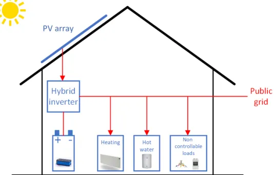
For the study of demand flexibility, a residential building was assumed that is located in Hungary. The building is equipped with an electric heating system, a separate water heater, a home energy storage system, and rooftop PV panels (see Figure1).
Figure 1.High-level model of the system. Line segments without arrow heads represent bidirectional power flow.
The prosumer model consisted of energy consumers (space heater, hot water, and noncontrollable load), a producer (PV), and a battery. The house was connected to the grid (on-grid mode), and power flow was available in both directions. All the energy needs of the house were supplied by the PV panels and the grid, and there was no other source of power (e.g., gas, central heating). Besides using energy from the grid, the PV panels and the battery can also supply the consumers. When available, self-consumption is preferred.
Instantaneous flexibility was calculated for all the devices in both directions and summed to provide a time series of the available flexibility.
A thermal model was developed for the space heating and hot water system. Not ev- ery electrical appliance can be controlled without inconveniencing consumers, so there are some appliances that consumers may always need access to. The flexibility of these appli- ances (e.g., lights, water, kitchen devices, other household appliances) was not considered in this study; their consumption is referred to as noncontrollable load. Power was supplied from the PV system, energy storage, or the grid. A conventional greedy algorithm was implemented to control energy storage operation when no external flexibility regulation was applied. The objective was to minimize grid usage.
There was no need for a separate flexibility control block in the case of the default operation scenario, when no external flexibility activation occurs. All the dispatchable devices could operate autonomously, and the greedy implementation of battery operation required no central control logic. Flexibility was calculated for each device, and the
sum represents the available flexibility of the house for both the up and down direction.
Flexibility followed the interpretation proposed by the authors of [28], i.e., it was assumed to be a signed value, positive when generation can be increased or consumption can be decreased and negative in the case when generation can be decreased or consumption can be increased.
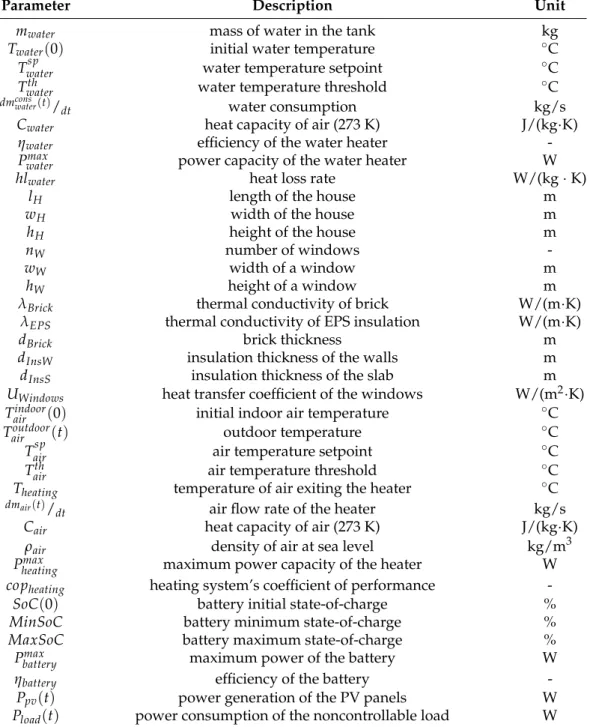
The residential house of the case study has the parameters presented in Table1.
Table 1.Exogenous variables of the system.
Parameter Description Unit
mwater mass of water in the tank kg
Twater(0) initial water temperature ◦C
Twatersp water temperature setpoint ◦C
Twaterth water temperature threshold ◦C
dmconswater(t)/dt water consumption kg/s
Cwater heat capacity of air (273 K) J/(kg·K)
ηwater efficiency of the water heater -
Pwatermax power capacity of the water heater W
hlwater heat loss rate W/(kg·K)
lH length of the house m
wH width of the house m
hH height of the house m
nW number of windows -
wW width of a window m
hW height of a window m
λBrick thermal conductivity of brick W/(m·K)
λEPS thermal conductivity of EPS insulation W/(m·K)
dBrick brick thickness m
dInsW insulation thickness of the walls m
dInsS insulation thickness of the slab m
UWindows heat transfer coefficient of the windows W/(m2·K)
Tairindoor(0) initial indoor air temperature ◦C
Tairoutdoor(t) outdoor temperature ◦C
Tairsp air temperature setpoint ◦C
Tairth air temperature threshold ◦C
Theating temperature of air exiting the heater ◦C
dmair(t)/dt air flow rate of the heater kg/s
Cair heat capacity of air (273 K) J/(kg·K)
ρair density of air at sea level kg/m3
Pheatingmax maximum power capacity of the heater W
copheating heating system’s coefficient of performance -
SoC(0) battery initial state-of-charge %
MinSoC battery minimum state-of-charge %
MaxSoC battery maximum state-of-charge %
Pbatterymax maximum power of the battery W
ηbattery efficiency of the battery -
Ppv(t) power generation of the PV panels W
Pload(t) power consumption of the noncontrollable load W 2.1. Hot Water
Hot water is supplied by an electric water tank containingmwaterkilograms of water.
A setpoint (Twatersp ) specifies the maximum temperature of the water, and a thermostat controls the heating cycles. The thermostat switches the heater off at the setpoint and turns it on (Equation (2)) when the temperature drops below the setpoint by a threshold value
(Twaterth ). When the heater is on, a heating wire warms up the water byηwater efficiently consuming a constant level of power (Pwater).
A water tank model calculates the water temperature dynamics (Equation (1)). The water temperature change (dTwaterdt(t)) has three main inputs: heat provided by the heater (dQ
gain water(t)
dt ), hot water consumption (dQconswaterdt (t)), and heat losses (dQheatlosswaterdt (t)). When hot water is consumed, the same amount of cold water (dmconswaterdt (t)) fills the tank. The inflow water temperature is the same as the outside temperature (Tairoutdoor(t)); thus, consumption cools the tank. The heat outflow is proportional to the temperature difference between the cold and the tank water (Twater(t)). Heat loss is calculated considering a heat loss parameter (hlwater) [34] and the difference between water and room temperature (Tairindoor). The room temperature is an output signal of the heating subsystem.
The energy balance of the hot water subsystem is expressed by the following equations:
Conswater(t) =Pwatermax ·Regwater(t) dQgainwater(t)
dt =Conswater(t)·ηwater
dQconswater(t)
dt = (Twater(t)−Tairoutdoor(t))· dm
conswater(t)
dt ·Cwater (1)
dQheatlosswater (t)
dt = (Twater(t)−Tairindoor)·mwater·hlwater
dTwater(t)
dt = dQ
gain water(t)
dt −dQ
conswater(t)
dt −dQ
heatloss water (t)
dt
! 1 mwater·Cwater
whereConswater(t)stands for the actual water consumption of the house.
Regwater(t) =
(1 , when the water heater is on,
0 , when the water heater is off. (2) Power is a signed value. Pwater(t)is negative (consumption) when the heater is on (Regwater(t)):
Pwater(t) =−Conswater(t). (3)
The calculated flexibility can be defined for both the up and down direction between current power consumption and the maximum power capacity (down) or 0 (up) using (Equation (4)) below.
Fwaterup (t) =Conswater(t) (4)
Fwaterdown(t) =Conswater(t)−Pwatermax
2.2. Heating
The thermal model of a house calculates the power consumption of the heating system that keeps the indoor temperature around a defined setpoint. The heating system is equipped with a thermostat and an electric heater. Similar to the water heater, the thermostat switches the heater on and off (Equation (9)) when the temperature drops below and above the setpoint (Tairsp) by a predefined threshold (Tairth). An air-to-air heat pump supplies warm air for the house, operating at an average COP ratio (copheating).
Total thermal resistance (Rtot) is calculated from the geometry and the material prop- erties of the house (Equation (5)). The walls of the house are made of bricks, and EPS insulation is used on the walls and the slab.
AWindows=nW·hW·wW
AWalls=2·lH·hH+2·wH·hH−AWindows (5) ASlab=wH·lH
A= AWindows+AWalls+ASlab
The thermal resistance of thermally homogeneous components is calculated using (Equation (6)).
RWindows=1/UWindows
RWalls=dBrick/λBrick+dInsW/λEPS (6)
RSlab =dInsS/λEPS
The total thermal resistance (Rtot) is determined by assuming one-dimensional heat flow perpendicular to the walls. It is given (Equation (7)) by the method in the ISO 6946/2007 standard [35].
Rtot= A
AWalls/RWalls+AWindows/RWindows+ASlab/RSlab (7) A thermal model calculates the indoor air temperature dynamics of the house. Its two main inputs are the heat provided by the heating system and heat losses. Contrary to the water heater, heat gain (dQ
gain heating(t)
dt ) is not persistent, but proportional to the temperature difference between the room (Tairindoor) and the constant heated air temperature (Theating).
Heat loss (dQ
heatloss heating(t)
dt ) is proportional to the temperature difference between the room and outdoor temperature (Tairoutdoor). The indoor temperature time derivative (dTairindoordt (t)) is expressed by the following equations:
dQgainheating(t) dt =min
(Theating−Tairindoor(t))dmair(t)
dt Cair,Phpmaxcopheating
Regheating(t)
dQheatlossheating(t)
dt =Tairindoor(t)−Tairoutdoor(t) 1
RtotA (8)
dTairindoor(t)
dt =
dQgainheating(t)
dt − dQ
heatloss heating(t)
dt
1
(lH·wH·hH)·ρair·Cair
Regheating(t) =
(1 , when the heater is on,
0 , when the heater is off. (9)
Consheating(t)denotes a theoretical power consumption that is necessary to warm the indoor air up to the constant heated air temperature.
Consheating(t) =min (Theating−Tairindoor(t))dmairdt(t)Cair copheating
,Phpmax
!
(10)
Power is a signed value.Pheating(t)is negative (consumption) when the heater is on:
Pheating(t) =−Consheating(t)Regheating(t). (11) The available flexibility quantity from the heating system is calculated for both direc- tions (Equation (12)). When the heater is on, its power consumption can be decreased, and the maximum upward flexibility is the difference between instantaneous power and zero.
When it is off, downward regulation is available by turning the heater on.
Fheatingup (t) =Consheating(t)Regheating(t) (12) Fheatingdown (t) =−Consheating(t)(1−Regheating(t))
2.3. Storage
Storage provides the flexibility of shifting energy over time. A conventional greedy algorithm was implemented to control the storage operation when no external flexibility regulation was applied [36] in order to prefer self-consumption and reduce feed-in power.
If there is a higher consumption by the household than generation by the PV, the storage is discharged until a minimum charge level. When generation surplus occurs, the storage is charged until it is full.
The storage model (Equations (13)–(16)) processes the power requirement (Regbattery(t)), determines the default storage operation (charge:Conschargebattery(t)/discharge:Consdischargebattery (t)), and calculates current state-of-charge (SoC(t)) taking into consideration the power limits (Pbatterymax ), capacity limits (MinSoC,MaxSoC), and efficiency ratio (ηbattery).
Regbattery(t) =Pwater(t) +Pheating(t) +Pload(t) +Ppv(t) (13)
Conschargebattery(t) =
(min(max(0,Regbattery(t)),Pbatterymax ), whenSoC(t)<MaxSoC,
0, otherwise (14)
Consdischargebattery (t) =
(max(min(0,Regbattery(t)),−Pbatterymax ), SoC(t)> MinSoC,
0, otherwise (15)
dSoC(t)
dt = Cons
charge
battery(t)·ηbattery+Consdischargebattery (t)·(2−ηbattery)
Cap (16)
The battery’s contribution to the net power balance of the house (Pbattery(t)) has the opposite sign of battery consumption.
Pbattery(t) =−Conschargebattery(t)−Consdischargebattery (t) (17) Given the maximum charge (Pbatterymax ) and discharge (Pbatterymin ) power of the energy storage and the instantaneous power output, both up and down regulation capacity can be calculated (Fbatteryup (t),Fbatterydown (t)) when the state-of-charge is between the charge limits.
Fbatteryup (t) =Pbatterymax −Pbattery(t) (18) Fbatterydown (t) =−Pbatterymax −Pbattery(t)
2.4. Noncontrollable Load
The consumption of the household is made up of controllable and noncontrollable loads. While the controllable load was presented in the previous sections, the measured data were used for the noncontrollable load time series (Pload(t)). No flexibility was available for the noncontrollable load.
2.5. PV Generation
PV generation (Ppv(t)) depends only on solar radiation. When no flexibility control was applied, it was assumed that the panels always generated the maximum power, and no upward regulation was available. The PV can offer downward flexibility (Fpvdown(t)) between 0 and its current generation.
Fpvdown(t) =−Ppv(t) (19) 2.6. Power Balance and Total Flexibility
The power balance of the house is calculated by summarizing the signed values of each component.
Pbalance(t) =Pwater(t) +Pheating(t) +Pbattery(t) +Pload(t) +Ppv(t) (20) The total flexibility is calculated separately for the up and down direction:
Ftotalup (t) =Fwaterup (t) +Fheatingup (t) +Fbatteryup (t)
Ftotaldown(t) =Fwaterdown(t) +Fheatingdown (t) +Fbatterydown (t) +Fpvdown(t) (21) 2.7. Model Verification
The simulation parameters were configured taking the geometry and materials used in the well-insulated, single-story residential house built in 2015 in Hungary. The building has a ground floor area of 172 m2, made of insulated brick (38 + 15 cm). The ceiling has a concrete structure with 30 cm of insulation. The windows have three-pane thermal insulated glazing.
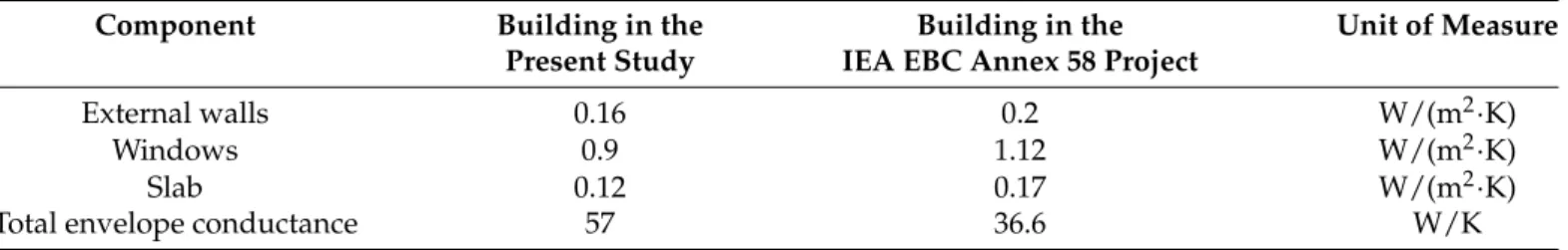
The parameters and calculated variables were compared to the values of the single- family house involved in the IEA EBC Annex 58 project [37]. The referenced building area is 100 m2; its brick walls are insulated, and double-pane windows were built in. The benchmark building has slightly worse U-values [38], but the total conductance is lower, because of the difference in size. Interior walls were also considered in the thermodynamic calculations. The comparisons of the heat transfer coefficients are given in Table2.
Table 2.Calculated heat transfer coefficients.
Component Building in the Building in the Unit of Measure
Present Study IEA EBC Annex 58 Project
External walls 0.16 0.2 W/(m2·K)
Windows 0.9 1.12 W/(m2·K)
Slab 0.12 0.17 W/(m2·K)
Total envelope conductance 57 36.6 W/K
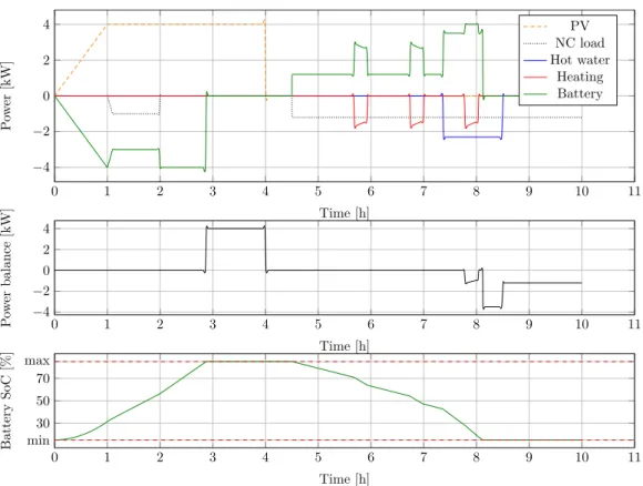
The model was tested with manual inputs. Figure2shows the model response for an arbitrarily chosen input set. In the beginning, there was no consumption. PV generation ramped up to 4 kW. It charged the battery and supplied the load between one and two.
The power balance of the house remained zero until the battery was full. At Hour 5, the outdoor temperature dropped to−2◦C from 24◦C, making the space heater turn on after 40 min. Between Hours 6 and 8, 6 L/min hot water was also used. The battery supplied
the noncontrollable load and the consumption of both heaters until the SoC reached its minimum level. The building was fed from the grid after Hour 8. It can be concluded that the proposed simulation model corresponded to the engineering expectations.
0 1 2 3 4 5 6 7 8 9 10 11
−4
−2 0 2 4
Time [h]
Power[kW]
PV NC load Hot water
Heating Battery
0 1 2 3 4 5 6 7 8 9 10 11
−4
−2 0 2 4
Time [h]
Powerbalance[kW]
0 1 2 3 4 5 6 7 8 9 10 11
min 30 50 70 max
Time [h]
BatterySoC[%]
Figure 2.Power of the devices for the verification inputs.
2.8. Flexibility Prediction
The quantification of the flexibility provides instant volumes of the up and down regulation capabilities. Instantaneous values are not valuable for flexibility buyers such as system operators, so forecasts need to be calculated. It was not a primary objective of this paper to study the prediction methods and evaluate the results; however, a simple forecast model was built to show the short-term prediction opportunities.
A linear model was fit to minimize the residual sum of squares between the observed features and the values predicted by the linear approximation. Ridge regression was used, which kept all predictors in the model, but performed an L2-norm regularization, reducing the impact of correlated predictors. Ridge regression is a regularized version of linear regression where a regularization term is added to the cost function. This forces the learning algorithm to not only fit the data, but also keep the model weights smaller in magnitude [39]. The objective function of RR is defined as follows [40]:
minw
1 2
∑
n i=1||wTxi−yi||22+λ||w||22, (22) where xi is the feature vector of thei-th sample andyi is the independent variable’s true value. λis a regularization parameter. Weight vectorwis calculated by taking the derivative of Equation (22) and setting it to zero.
w= (X XT+λI)−1XyT (23) A 15 min interval is the typical market time unit for settlement in the energy sector in Europe. The calculation of a 15 min forecast of upward flexibility assumes that it has a linear relationship between upward flexibility (yi) and the predictor variables (xi). PV
generation, heating system/water heater consumption, power, and the state-of-charge of the battery were selected as the explanatory variables. There was no prediction of the features, so 15 min lags were applied to construct the predictor set (Equation (25)). A 15 min average of the target variable was calculated and lagged by 15 min (Equation (24)).
Flexuprolling(i) =∑
i−900300
t=i−18001200Ftotalup (t)
900 (24)
xi =
Pwater(i−900) Pheating(i−900) Pbattery(i−900) Ppv(i−900) SoC(i−900) Flexuprolling(i)
(25)
Ridge regression puts constraints on the size of the coefficients associated with each variable. These values depend on the magnitude of each variable. If a variable is measured at a higher scale than the other variables and not centered around zero, they do not give an equal contribution to the analysis. Both the training and test set must be standardized based on the mean and standard deviation learned from the training set by removing the mean and scaling data to unit variance as follows:
z= x−µ
σ , (26)
whereµis the mean,σis the standard deviation ofx, andzis the scaled predictors.
The coefficient of variation of the root-mean-squared error (CVRMSE) and the coeffi- cient of determination (R2score) were used as a set of criteria to evaluate the prediction.
The CVRMSE (Equation (27)) measures the variability of errors between true and predicted values. It gives an indication of the model’s ability to predict the overall load shape that is reflected in the data [41].
CVRMSE(y, ˆy) = 1 1
n∑ni=1yi s1
n
∑
n i=1(yi−yˆi)2100 (27)
R2(28) represents the proportion of variance that has been explained by the indepen- dent variables in the model. It provides an indication of the goodness of fit and therefore a measure of how well unseen samples are likely to be predicted by the model, through the proportion of explained variance [42].
R2(y, ˆy) =1−∑
ni=1(yi−yˆi)2
∑ni=1(yi−y¯)2, (28) where:
• n: number of samples;
• yi: true value;
• yˆi: predicted value of the i-th sample;
• y¯= 1n∑ni=1yi.
3. Case Study and Results 3.1. Scenarios
The energy model of the house in Section2was implemented in MATLAB Simulink.
It calculated the total power consumption/generation and available flexibility that it could offer. Four simulations were performed to analyze flexibility under different weather conditions and patterns for a 24 h period. The scenarios differed in the PV generation and
outer temperature time series data, and it was assumed that the noncontrollable load and water consumption patterns were the same in each scenario. Please refer to AppendixAto review additional parameter values.
Figure3shows the difference between the solar generation profile for the different scenarios. The 1 min measurements from a 400 kVA PV park were collected and normalized by the peak power capacity. The relative production of each scenario was multiplied by the capacity of the modeled rooftop panels to obtain the PV generation time series (Ppv(t)).
4 6 8 10 12 14 16 18 20 22
0 1 2 3
Time [h]
PVgeneration[kW]
Winter, sunny Winter, cloudy Summer, sunny Summer, cloudy
Figure 3.PV generation profiles for the four scenarios. The higher generation at 8 a.m. on a cloudy summer day (red line) compared to a sunny summer day (orange, dashed) comes from the efficiency increase caused by the cooling (a possible cloud passing by) at 7 a.m.
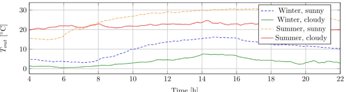
Figure4shows the environmental temperature (Tout) for the different scenarios. Tem- perature data were collected from the PV site (Tairoutdoor(t)).
4 6 8 10 12 14 16 18 20 22
0 10 20 30
Time [h]
Tout[◦C]
Winter, sunny Winter, cloudy Summer, sunny Summer, cloudy
Figure 4.Outer temperature profiles for the four scenarios.
The Almanac of Minutely Power dataset (AMPds) [43] contains electricity, water, and natural gas measurements at one minute intervals for two years of monitoring. There is a total of twenty-one power meters and two water meters installed in a residential house similar to the one analyzed in this study. The 21 electronic submeters were assigned to groups: controllable and noncontrollable devices. Controllable devices consist of the HVAC, heat pump, and hot water heater, and noncontrollable group contains bedroom, basement, dining room plugs and lights, clothes washer and dryer, dishwasher, kitchen fridge and oven, garage, home office, entertainment, utility room, and outside plugs. All noncontrollable measurements were added, and a typical 1 d time series was created by calculating the average value of the same minute for every day of the two-year monitoring period. Figure5shows the noncontrollable consumption for all the scenarios (Pload(t)).
0 2 4 6 8 10 12 14 16 18 20 22 24
−0.6
−0.4
−0.2
Time [h]
Consumption[kW]
NC load
Figure 5.Noncontrollable electrical load for the four different scenarios.
Hot water consumption (Figure6) was calculated by the same method as the non- controllable load. The Almanac of Minutely Power dataset was the source of the 1 min consumption data. The mean value was calculated for every minute of the day to generate a 1 d normal water consumption (dmconswater(t)/dt).
0 2 4 6 8 10 12 14 16 18 20 22 24
0 20 40
Time [h]
Waterflow[l/min]
Hot water consumption
Figure 6.Hot water consumption for the four different scenarios.
3.2. Simulation Results for the Scenarios 3.2.1. Winter—Sunny Day
Figure7shows the power consumption and generation of the simulated devices.
Supply from the grid and PV generation was the primary sources of energy. Net power is the balance of the house; it is the volume of power consumption from or fed to the grid. When the PV generates sufficient power to feed all consumption units, the energy surplus charges the battery. The greedy battery control method discharges the storage when the PV is low. After 8 p.m., the house is supplied from the grid again, after the battery becomes empty.
The band of flexibility was not symmetric: although the house was a prosumer, generation and storage capacity was limited, and consumption was intermittent. There was more time when a consumption device could be turned on than off, so the downward flexibility was higher. PV generation increased the upward flexibility by charging the battery: the battery consumption could always be switched to production.
4 6 8 10 12 14 16 18 20 22 24
−2 0 2 4
Time [h]
Power[kW]
PV NC load Hot water
Heating Battery
4 6 8 10 12 14 16 18 20 22 24
−4
−2 0
Time [h]
Powerbalance[kW]
4 6 8 10 12 14 16 18 20 22 24
min 30 50 70 max
Time [h]
BatterySoC[%]
Figure 7.Power consumption/generation of devices for the winter sunny day scenario.
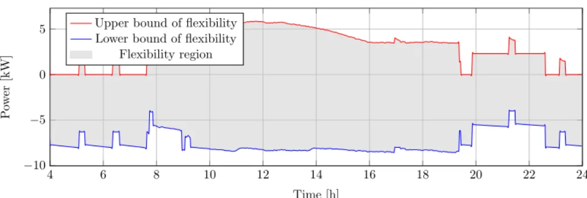
The upward and downward flexibility capabilities of each device were added, result- ing in the building’s maximum flexible power (Figure8).
4 6 8 10 12 14 16 18 20 22 24
−10
−5 0 5
Time [h]
Power[kW]
Upper bound of flexibility Lower bound of flexibility
Flexibility region
Figure 8.Available upward and downward flexibility for the winter sunny day scenario.
3.2.2. Winter—Cloudy
Figure9shows the power consumption and generation of the simulated devices. On a cloudy winter day, the effect of self-generation was limited, and upward flexibility was confined to the short periods when consumption devices operate or the PV is able to supply the house and charge the battery. The downward direction was not affected.
4 6 8 10 12 14 16 18 20 22 24
−2 0 2
Time [h]
Power[kW]
PV NC load Hot water
Heating Battery
4 6 8 10 12 14 16 18 20 22 24
−4
−2 0
Time [h]
Powerbalance[kW]
4 6 8 10 12 14 16 18 20 22 24
min 30 50 70 max
Time [h]
SoC[%]
Figure 9.Power consumption/generation of devices for the winter cloudy day scenario.
The upward and downward flexibility capabilities of each device were added, result- ing in the building’s maximum flexible power (Figure10).
4 6 8 10 12 14 16 18 20 22 24
−5 0 5
Time [h]
Power[kW]
Upper bound of flexibility Lower bound of flexibility
Flexibility region
Figure 10.Available upward and downward flexibility for the winter cloudy day scenario.
3.2.3. Summer—Sunny
Figure11shows the power consumption and generation of the simulated devices.
On a sunny summer day, the PV generation had a major effect: together with the storage, self-production was sufficient to supply the instantaneous power consumption of the house.
After noon, the generation surplus was fed back to the grid.
4 6 8 10 12 14 16 18 20 22 24
−2 0 2
Time [h]
Power[kW]
PV NC load Hot water
Heating Battery
4 6 8 10 12 14 16 18 20 22 24
0 1 2
Time [h]
Powerbalance[kW]
4 6 8 10 12 14 16 18 20 22 24
min 30 50 70 max
Time [h]
SoC[%]
Figure 11.Power consumption/generation of devices for the summer sunny day scenario.
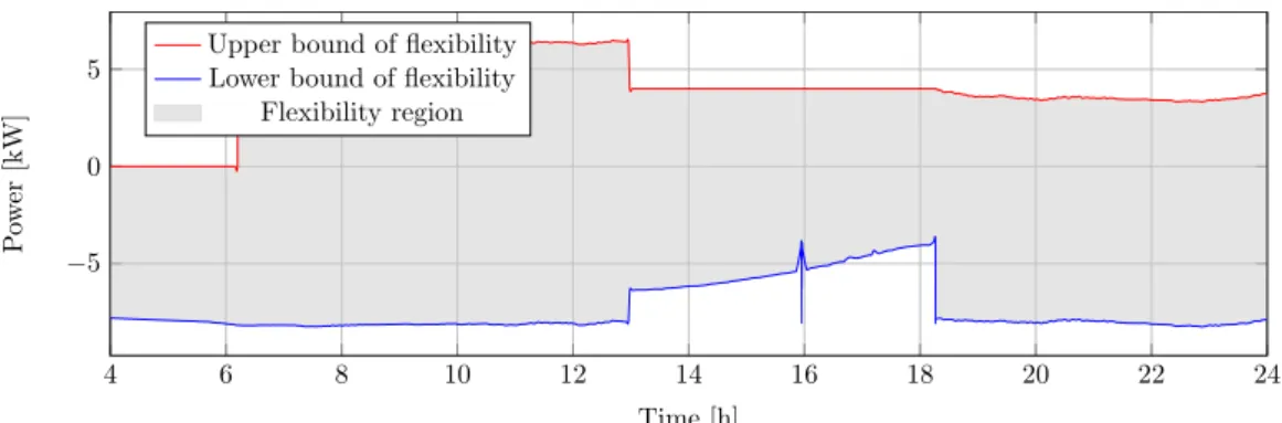
The upward and downward flexibility capabilities of each device were added, result- ing in the building’s maximum flexible power (Figure12).
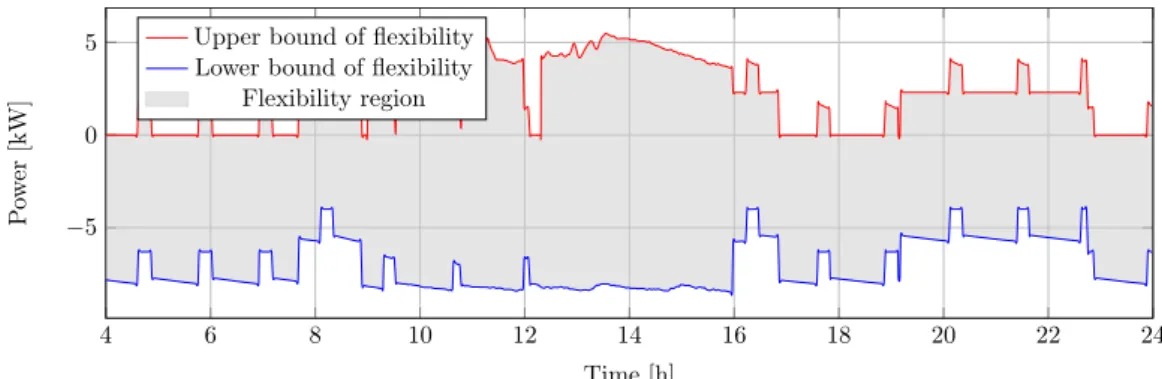
3.2.4. Summer—Cloudy
Figure13shows the power consumption and generation of the simulated devices.
A cloudy summer day resulted in a more variable upward flexibility in the positive direc- tion. The energy of PV production was not enough to supply the house all day, but 90% of the time, so there was no grid usage.
4 6 8 10 12 14 16 18 20 22 24
−5 0 5
Time [h]
Power[kW]
Upper bound of flexibility Lower bound of flexibility
Flexibility region
Figure 12.Available upward and downward flexibility for the summer sunny day scenario.
4 6 8 10 12 14 16 18 20 22 24
−2 0 2
Time [h]
Power[kW]
PV NC load Hot water
Heating Battery
4 6 8 10 12 14 16 18 20 22 24
−3
−2
−1 0
Time [h]
Powerbalance[kW]
4 6 8 10 12 14 16 18 20 22 24
min 30 50 70 max
Time [h]
SoC[%]
Figure 13.Power consumption/generation of devices for the summer cloudy day scenario.
The upward and downward flexibility capabilities of each device were added, result- ing in the building’s maximum flexible power (Figure14).
4 6 8 10 12 14 16 18 20 22 24
−5 0 5
Time [h]
Power[kW]
Upper bound of flexibility Lower bound of flexibility
Flexibility region
Figure 14.Available upward and downward flexibility for the summer cloudy day scenario.
3.2.5. Prediction
The previous sections presented prosumer flexibility in different environmental condi- tions for 1 d. Here, the results of the forecast model (Section2.8) are shown based on one month of one-minute resolution input data for the upward direction. The simulation of the flexibility represents the true value of the target variable. One-third of the one-month input interval was held back as a test to provide an unbiased evaluation of the model fit on the training dataset.
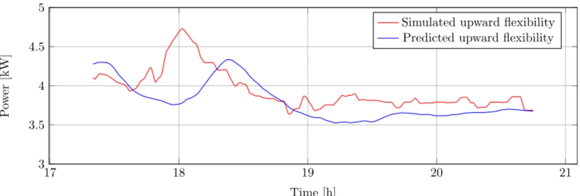
The ridge regression model generates the target variable of the linear forecast model, that is the 15 min forecast of up and down flexibility. Prediction on the test set provided a 25.5% CVRMSE and a 0.89 R2 score. Figure15shows a 4 h sample of the prediction.
17 18 19 20 21
3 3.5 4 4.5 5
Time [h]
Power[kW]
Simulated upward flexibility Predicted upward flexibility
Figure 15.Sample from the upward flexibility prediction between 17:20 and 20:45.
The predictors explained the target variable well; however, the variability of the errors was high given the short forecast interval.
3.3. Discussion of the Results
Applying measured weather and load data, the experiments were performed along four different, but typical scenarios. The results showed that the highest range of flexibility was available in the summer time, when there was no heating and the solar generation was maximal. It was also clear that the battery usage was higher in the summer, when the solar generation was not being consumed instantly. It is important to note that a properly sized air conditioner unit would balance the load between the summer and winter periods.
4. Conclusions
Demand-side flexibility can be a valuable source for system operators; however, residential prosumers do not follow a well-defined schedule, so a firm volume of available flexibility cannot be planned, but predicted. A flexibility framework was proposed in this paper for residential prosumers in a distributed generation setup. The residential prosumer of the case study was parameterized so that it described a usual residential actor of the system. To quantify building demand flexibility, the thermoelectric dynamic response of the building energy system was modeled and implemented in MATLAB Simulink. Power consumption and generation were modeled. Simulations were performed based on real world data, and the flexibility potential was calculated for both up and down flexibility.
The simulation of four scenarios was executed, which covered one day in different seasons.
Power consumption and generation were calculated, as well as upward and downward instantaneous flexibility.
A ridge-regression-based prediction method was designed, and the short-term forecast was calculated. The simulation and prediction experiments showed that the proposed method could serve as the basis of a state estimator or prediction unit. The accuracy of the forecast was moderate, but by assessing different prediction methods on the prosumer flexibility model, we could choose the right tool to improve accuracy and confidence of the prediction.
The aggregation of prosumers’ flexibility is necessary to reach the volume that a system operator can utilize. The framework presented forms a basis to analyze the flexibility prediction opportunities on aggregated prosumer portfolios.
The future research directions include the generalization of the method to a higher number of households, for example a local transformer area, in order to give an estimate of the flexibility of a group of prosumers. Another step in the development of the proposed method is to use novel prediction methods from the field of data science to enhance the short-term prediction performance for flexibility.
Author Contributions: Conceptualization, I.G.B.; software, I.G.B.; validation, I.G.B. and A.M.;
writing—original draft preparation, I.G.B.; writing—review and editing, A.F. and A.M.; visual- ization, A.M.; supervision, A.M. and A.F. All authors read and agreed to the published version of the manuscript.
Funding:Project No. 131501 was implemented with the support provided from the National Re- search, Development and Innovation Fund of Hungary, financed under the K_19 funding scheme.
A.M. was supported by the János Bolyai Research Scholarship of the Hungarian Academy of Sci- ences. A.M. was supported by the ÚNKP-20-5 new national excellence program of the Ministry for Innovation and Technology.
Institutional Review Board Statement:Not applicable.
Informed Consent Statement:Not applicable.
Conflicts of Interest:The authors declare no conflict of interest. The funders had no role in the design of the study; in the collection, analyses, or interpretation of data; in the writing of the manuscript;
nor in the decision to publish the results.
Sample Availability:The Simulink model of the case study is available from the authors. The AMPds dataset is openly available athttps://doi.org/10.7910/DVN/FIE0S4(Date of access: 10 December 2020) and licensed under a Creative Commons Attribution 4.0 International License. The operator of the PV site did not agree to have their data shared publicly, so the PV generation and outdoor temperature data are not available. The energy audit document of the building is not available.
Abbreviations
The following abbreviations are used in this manuscript:
COP Coefficient of performance
CVRMSE Coefficient of variation of the root-mean-squared error
DR Demand response
DG Distributed generation DSM Demand-side management DHW Domestic hot water EPS Expanded polystyrene HEM Home energy management
HP Heat pump
HVAC Heating, ventilating, and air conditioning
PV Photovoltaic
SoC State-of-charge
TSO Transmission system operator DSO Distribution system operator
Appendix A
The simulation parameters were taken from the energy audit of a residential building located in Hungary. Together with the house geometry, they are referred to as the “house parameters”. The authors determined additional simulation values considering the typical configuration or characteristics of the devices.
Table A1.Simulation parameters.
Parameter Value Unit of Measure Source
lH 22 m House parameter
wH 10 m House parameter
hH 3 m House parameter
nW 7 m House parameter
wW 1 m House parameter
hW 1.6 m House parameter
λBrick 0.179 W/(m·K) House parameter
λEPS 0.035 W/(m·K) House parameter
dBrick 0.38 m House parameter
dInsW 0.15 m House parameter
dInsS 0.3 m House parameter
UWindows 0.9 W/(m2*K) House parameter
mwater 120 kg Determined by the authors
Twater(0) 55 ◦C Determined by the authors
Twatersp 65 ◦C Determined by the authors
Twaterth 15 ◦C Determined by the authors
Cwater 4181 J/(kg·K) Physical constant
ηwater 0.9 - Determined by the authors
Pwatermax 2300 W Determined by the authors
hlwater 0.0069 W/(kg·K) Derived from the results of [34]
Tairindoor(0) 24 ◦C Determined by the authors
Tairsp 22 ◦C Determined by the authors
Tairth 3 ◦C Determined by the authors
Theating 50 ◦C Determined by the authors
dmair(t)/dt Constant 0.2 kg/s Determined by the authors
Cair 1005.4 J/(kg·K) Physical constant
ρair 1.225 kg/m3 Physical constant
Pheatingmax 10,000 W Determined by the authors
copheating 3.6 - Determined by the authors
SoC(0) 15 % Determined by the authors
MinSoC 15 % Determined by the authors
MaxSoC 85 % Determined by the authors
Pbatterymax 4000 W Determined by the authors
ηbattery 0.9 - Determined by the authors
References
1. Saleh, S.A.; Pijnenburg, P.; Castillo-Guerra, E. Load Aggregation from Generation-Follows-Load to Load-Follows-Generation:
Residential Loads. IEEE Trans. Ind. Appl.2017,53, 833–842. [CrossRef]
2. Merino, J.; Gómez, I.; Turienzo, E.; Madina, C.Ancillary Service Provision by RES and DSM Connected at Distribution Level in the Future Power System; Technical Report; SmartNet project D: Donostia-San Spain, 2016.
3. Bálint, R.; Fodor, A.; Magyar, A. Model-Based Power Generation Estimation of Solar Panels Using Weather Forecast for Microgrid Application.Acta Polytech. Hung.2019,16, 149–165.
4. Kirbas, I.; Kerem, A. Short-Term Wind Speed Prediction Based on Artificial Neural Network Models. Meas. Control2016, 49, 183–190. [CrossRef]
5. Qian, Z.; Pei, Y.; Zareipour, H.; Chen, N. A Review and Discussion of Decomposition-Based Hybrid Models for Wind Energy Forecasting Applications. Appl. Energy2019,235, 939–953. [CrossRef]
6. Gissey, G.C.; Subkhankulova, D.; Dodds, P.E.; Barrett, M. Value of Energy Storage Aggregation to the Electricity System. Energy Policy2019,128, 685–696. [CrossRef]
7. García Vera, Y.E.; Dufo-López, R.; Bernal-Agustín, J.L. Energy Management in Microgrids with Renewable Energy Sources:
A Literature Review.Appl. Sci.2019,9, 3854. [CrossRef]
8. European Commission. Proposal for a Directive of the European Parliament and of the Council on Common Rules for the Internal Market in Electricity; Council of the European Union: Brussels, Belgium, 2017.