, Mohamed Ben Alaya

Asymptotic behavior of maximum likelihood estimators for a jump-type Heston model

M´ aty´ as Barczy

, Mohamed Ben Alaya

, Ahmed Kebaier

and Gyula Pap

* MTA-SZTE Analysis and Stochastics Research Group, Bolyai Institute, University of Szeged, Aradi v´ertan´uk tere 1, H–6720 Szeged, Hungary.

** Laboratoire De Math´ematiques Rapha¨el Salem, UMR 6085, Universit´e De Rouen, Avenue de L’Universit´e Technopˆole du Madrillet, 76801 Saint-Etienne-Du-Rouvray, France.

*** Universit´e Paris 13, Sorbonne Paris Cit´e, LAGA, CNRS (UMR 7539), Villetaneuse, France.

**** Bolyai Institute, University of Szeged, Aradi v´ertan´uk tere 1, H–6720 Szeged, Hungary.

e–mails: barczy@math.u-szeged.hu (M. Barczy),

mohamed.ben-alaya@univ-rouen.fr (M. Ben Alaya), kebaier@math.univ-paris13.fr (A. Kebaier),

papgy@math.u-szeged.hu (G. Pap).

Corresponding author

Abstract

We study asymptotic properties of maximum likelihood estimators of drift parameters for a jump-type Heston model based on continuous time observations, where the jump process can be any purely non-Gaussian L´evy process of not necessarily bounded varia- tion with a L´evy measure concentrated on (−1,∞). We prove strong consistency and asymptotic normality for all admissible parameter values except one, where we show only weak consistency and mixed normal (but non-normal) asymptotic behavior. It turns out that the volatility of the price process is a measurable function of the price process. We also present some numerical illustrations to confirm our results.

1 Introduction

Parameter estimation, especially studying asymptotic properties of maximum likelihood esti- mator (MLE) of drift parameters for Cox–Ingersoll–Ross (CIR) and Heston models is an active

2010 Mathematics Subject Classifications: 60H10, 91G70, 60F05, 62F12.

Key words and phrases: jump-type Heston model, maximum likelihood estimator.

This research is supported by Laboratory of Excellence MME-DII, Grant no. ANR11-LBX-0023-01 (http://labex-mme-dii.u-cergy.fr/). M´aty´as Barczy was supported between September 2016 and Jan- uary 2017 by the ”Magyar ´Allami E¨otv¨os ¨Oszt¨ond´ıj 2016” Grant no. 75141 funded by the Tempus Public Foundation, and from September 2017 by the J´anos Bolyai Research Scholarship of the Hungarian Academy of Sciences. Ahmed Kebaier benefited from the support of the chair ”Risques Financiers”, Fondation du Risque.

arXiv:1509.08869v4 [math.ST] 18 May 2018

area of research mainly due to the wide range of applications of these models in financial mathematics.

The present paper gives a new contribution to the theory of asymptotic properties of MLE for jump-type Heston models based on continuous time observations. Concerning related works, due to the vast literature on parameter estimation for Heston models, we will restrict ourselves to mention only papers that investigate the very same types of questions. For a detailed and recent survey on parameter estimation for Heston models in general, see the Introduction of Barczy and Pap [6].

Overbeck [33] studied MLE of the drift parameters of the first coordinate process of a (diffusion type) Heston model (see (1.1)) based on continuous time observations, which is nothing else but a CIR process, also called square root process or Feller process. Ben-Alaya and Kebaier [8], [9] made a progress in MLE for the CIR process, giving explicit forms of joint Laplace transforms of the building blocks of this MLE as well.

Barczy and Pap [6] considered a Heston model (dY_t= (a−bY_t) dt+σ₁√

Y_tdW_t, dX_t = (α−βY_t) dt+σ₂√

Y_t %dW_t+p

1−%²dB_t

, t ∈[0,∞), (1.1)

where a, σ₁, σ₂ ∈ (0,∞), b, α, β ∈ R, % ∈ (−1,1) and (W_t, B_t)_t∈[0,∞) is a 2-dimensional standard Wiener process. Here (X_t)t∈[0,∞) is the log-price process of an asset, (Y_t)t∈[0,∞) is its stochastic volatility (or instantaneous variance), σ₁ ∈ (0,∞) is the so-called volatility of the volatility, and % ∈ (−1,1) is the correlation between the driving standard Wiener processes (W_t)t∈[0,∞) and (%W_t+p

1−%²B_t)t∈[0,∞). The MLE of the drift parameters (a, b, α, β) and its asymptotic behavior have been investigated based on continuous time observations (Y_t, X_t)_t∈[0,T] with T ∈(0,∞) for all admissible parameter values (according to b >0, b= 0, and b <0). It turned out that, for all t ∈[0, T], Y_t is a measurable function of (X_t)t∈[0,T], hence, for the calculation of the MLE in question, one does not need the sample (Y_t)t∈[0,T].

The original Heston model (see Heston [18]) takes the form (dY_t=κ(θ−Y_t) dt+σ√

Y_tdW_t, dS_t =µS_tdt+S_t√

Y_t %dW_t+p

1−%²dB_t

, t∈[0,∞), (1.2)

where (S_t)_t∈[0,∞) is the price process of an asset, µ ∈ R is the rate of return of the asset, θ ∈ (0,∞) is the so-called long variance (long run average price variance, i.e., the limit of E(Y_t) as t → ∞), κ∈(0,∞) is the rate at which (Y_t)t∈[0,∞) reverts to θ, and σ∈(0,∞) is the so-called volatility of the volatility. We call the attention that there are two differences between the models (1.1) and (1.2). Namely, in (1.2) the coefficient κ can only be positive, while in (1.1) the corresponding coefficient b can be an arbitrary real number. In other words, the first coordinate process in (1.1) can be subcritical, critical or supercritical (according to b >0, b = 0, and b <0), but in (1.2) it can only be subcritical (since κ >0). Moreover, the second coordinate process in (1.2) is the price process, while in (1.1) it is the log-price process.

In this paper we study a jump-type Heston model (also called a stochastic volatility with jumps model, SVJ model)

(dY_t=κ(θ−Y_t) dt+σ√

Y_tdW_t, dS_t =µS_tdt+S_t√

Y_t %dW_t+p

1−%²dB_t

+S_t−dL_t, t ∈[0,∞), (1.3)

where (L_t)t∈[0,∞) is a purely non-Gaussian L´evy process independent of (W_t, B_t)t∈[0,∞) with L´evy–Khintchine representation

(1.4) E(e^iuL1) = exp

iγu+ Z ∞

−1

(e^iuz −1−iuz1(−1,1](z))m(dz)

, u∈R,

where γ ∈R and m is a L´evy measure concentrated on (−1,∞) with m({0}) = 0. Here, let us recall that the L´evy process L has finite variation on each interval [0, t], t ∈[0,∞), if and only if R1

−1|z|m(dz)<∞, see, e.g., Sato [35, Theorem 21.9]. We point out that the assumption P(Y₀ ∈ [0,∞), S₀ ∈ (0,∞)) = 1 and the assumption in question on the support of the L´evy measure m assure that P(St ∈(0,∞) for all t∈[0,∞)) = 1 (see Proposition 2.1), so the process S can be used for modeling prices in a financial market. From the point of view of financial mathematics, a natural question may occur concerning the model (1.3). Namely, is the drift coefficient of the second SDE in (1.3) well-adjusted in the sense that the discounted price process forms a martingale under some suitable equivalent martingale measure? We renounce to consider this question, we just note that one may have to choose the parameter µ in an appropriate way to assure this property. In Lamberton and Lapeyre [27, Section 7] one can find a detailed discussion of the same type of question for a jump-type Black-Scholes model, where the jumps of the log-price process is modeled by a compound Poisson process. They derived a necessary and sufficient condition for the drift coefficient of the underlying SDE in terms of the discounting factor and the parameters of the compound Poisson process in question in order that the discounted price process is a martingale, see [27, page 146]. For a good survey on jump-type Heston models, pricing and hedging in these models, see Runggaldier [34]. In fact, the model (1.3) is quite popular in finance with the special choice of the L´evy process L as a compound Poisson process. Namely, let

L_t:=

πt

X

i=1

(e^Ji −1), t∈[0,∞), (1.5)

where (π_t)_t∈[0,∞) is a Poisson process with intensity λ ∈ (0,∞), (J_i)i∈N is a sequence of independent identically distributed random variables having no atom at zero (i.e., P(J₁ = 0) = 0), and being independent of π as well. We also suppose that π, (J_i)i∈N, W and B are independent. One can interpret J as the jump size of the logarithm of the asset price. Then

E(e^iuL1) = exp

λ Z ∞

−1

(e^iuz−1)m(dz)

= exp

iuλ Z 1

−1

z m(dz) +λ Z ∞

−1

(e^iuz −1−iuz1[−1,1](z))m(dz)

, u∈R,

has the form (1.4) with m being the distribution of e^J1−1 and γ =λR1

−1z m(dz). Moreover, S_t takes the form

S_t=S₀exp Z t

0

µ−1

2Y_u du+

Z t 0

pY_u(%dW_u+p

1−%²dB_u) +

πt

X

i=1

J_i (1.6)

for t∈[0,∞), see (2.1). We note that the SDE (1.3) with the L´evy process L given in (1.5) has been studied, e.g., by Bates [7, equation (1)], Bakshi et al. [3, equations (1) and (2) with R≡0], by Broadie and Kaya [12, equations (30)-(31)] (where a factor St− is missing from the last term of equation (30)), by Runggaldier [34, Remark 3.1 with λt≡λ] and by Sun et al. [37, equation (1) withJ_v = 0]. Bates [7], Bakshi et al. [3] and Broadie and Kaya [12] have chosen the common distribution of J as a normal distribution. Bakshi et al. [3] used this model for studying (European style) S&P 500 options, e.g., they derived a practically implementable closed-form pricing formula. Broadie and Kaya [12] gave an exact simulation algorithm for this model, further, they considered the pricing of forward start options in this model. Sun et al. [37] have chosen the common distribution of J as a normal distribution, a one-sided exponential distribution or a two-sided distribution, and they applied the Fourier-cosine series expansion method for pricing vanilla options under these jump-type Heston models.

The aim of this paper is to study the MLE of the parameter ψ:= (θ, κ, µ) for the model (1.3) based on continuous time observations (Y_t, S_t)_t∈[0,T] with T ∈(0,∞), starting the process (Y, S) from some deterministic initial value (y₀, s₀)∈(0,∞)² supposing that σ, %, γ and the L´evy measure m are known. Here we stress that under these assumptions, the underlying statistical space corresponding to the parameters (κ, θ, µ)∈(0,∞)²×R is identifiable, however it would not be true for the statistical space corresponding to the parameters (κ, θ, µ, γ) ∈ (0,∞)²×R². We call the attention that the MLE in question contains stochastic integrals with respect to L. We prove that, for all t∈[0, T], L_t is a measurable function (i.e., a statistic) of (S_t)t∈[0,T], by providing a sequence of measurable functions of (S_t)t∈[0,T] converging in probability to L_t, see Remark 2.4 (note that this sequence depends on γ and m as well).

Further, it turns out that Y_t for all t ∈ [0, T], and the parameters σ and % are also measurable functions of (S_t)t∈[0,T], see Remarks 2.5 and 2.6, respectively. Hence, for the calculation of the MLE in question, one needs only the sample (St)t∈[0,T], the parameter γ and the L´evy measure m (γ and mare needed for the reconstruction of (L_t)_t∈[0,T]). Though we do not need to estimate the parameters σ and %, it is worth mentioning that the market microstructure effects may cause serious damage to the approximation of σ and % given in Remark 2.6 and to the MLE of (θ, κ, µ) in case of high-frequency observations as in Zhang et al. [41]. This type of question can be another interesting topic for future research.

The paper is organized as follows. In Section 2, we prove that the SDE (1.3) has a pathwise unique strong solution (under some appropriate conditions), see Proposition 2.1, we recall a result about the existence of a unique stationary distribution and ergodicity for the process (Yt)t∈[0,∞) given by the first equation in (1.3), see Theorem 2.2. In Proposition 2.3, we derive a Grigelionis representation for the process (S_t)_t∈[0,∞). Further, we prove that for all t ∈[0, T], L_t and Y_t are measurable functions of (S_t)_t∈[0,T], and we justify why we do not estimate the

parameters σ and %, see Remarks 2.4, 2.5 and 2.6. Section 3 is devoted to study the existence and uniqueness of the MLE (bθ_T,bκ_T,µb_T) of (θ, κ, µ) based on observations (Y_t, S_t)t∈[0,T] with T ∈ (0,∞). In Proposition 3.2, under appropriate conditions, we prove the unique existence of (bθ_T,bκ_T,µb_T), and we derive an explicit formula for it as well, see (3.11). In Remark 3.5, we describe the connection with the so called score vector due to Sørensen [36] and the estimating equation due to Luschgy [31], [32] leading to the same estimator. In Section 4, we prove that the MLE of (θ, κ, µ) is strongly consistent if θ, κ∈(0,∞) with θκ∈ ^σ₂²,∞

, and weakly consistent if θ, κ ∈ (0,∞) with θκ = ^σ₂², see Theorem 4.1 and Remark 4.2, respectively.

Section 5 is devoted to investigate the asymptotic behaviour of the MLE of (θ, κ, µ). In Theorem 5.1, provided that θ, κ ∈ (0,∞) with θκ ∈ ^σ₂²,∞

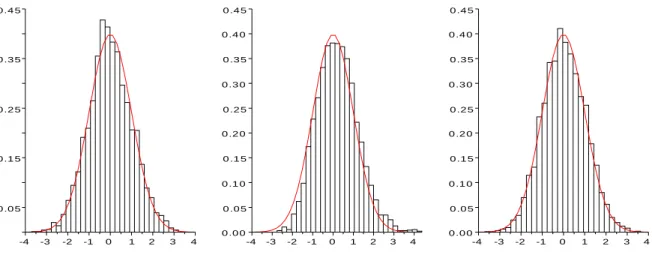
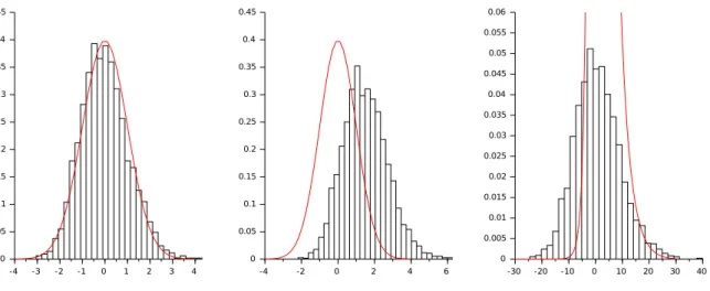
, we show that the MLE of (θ, κ, µ) is asymptotically normal with a usual square root normalization (T^1/2), but as usual, the asymptotic covariance matrix depends on the unknown parameters θ and κ, as well. To get around this problem, we also replace the normalization T^1/2 by a random one (depending only on the sample, but not on the parameters θ, κ and µ) with the advantage that the MLE of (θ, κ, µ) with the random scaling is asymptotically 3-dimensional standard normal. Theorem 5.3 is a counterpart of Theorem 5.1 in some sense. Namely, provided that θ, κ ∈ (0,∞) with θκ = ^σ₂², we derive two limit theorems for the MLE (bθ_T,bκ_T,bµ_T) with mixed normal limit distributions. First, we have a non-random scaling, but for µb_T instead of the usual scaling T^1/2 we have T; and then we have a random scaling as well. We point out that, surprisingly, the limit distributions in Theorems 5.1 and 5.3 do not depend on L (roughly speaking, they do not depend on the jump part). From a practical point of view, a natural question can occur, namely, how one can decide whether Theorems 5.1 and 5.3 can be applied (if yes, then which one), since one does not know the product θκ of the unknown parameters θ and κ in advance. To answer this question, one can build up a probe for testing the null hypothesis θκ = ^σ₂² against some alternative hypothesis, e.g., θκ > ^σ₂². In Section 6 we present some numerical illustrations of our limit theorems. We close the paper with Appendices, where we recall certain sufficient conditions for the absolute continuity of probability measures induced by semimartingales together with a representation of the Radon–

Nikodym derivative (Appendix A), some limit theorems for continuous local martingales for studying asymptotic behavior of (bθ_T,bκ_T,µb_T) (Appendix B) and a version of the continuous mapping theorem (Appendix C), and we give an explicit formula for the non-normal but mixed normal density function of the limit distribution of T(µb_T −µ) as T → ∞ in Theorem 5.3 (Appendix D).

We call the attention that in both cases θκ > ^σ₂² and θκ= ^σ₂², the CIR process Y has a unique stationary distribution and is ergodic, nevertheless, in case θκ > ^σ₂² the asymptotic limit distribution of the MLE of ψ = (θ, κ, µ) is normal, while in case θκ = ^σ₂² it is mixed normal. The interesting point is that we have an ergodic case with an asymptotically mixed normal (but non-normal) limit distribution. The main difference between the two ergodic cases is that E _Y¹_∞

<∞ if θκ > ^σ₂², but E _Y¹_∞

=∞ if θκ= ^σ₂².

2 Preliminaries

The next proposition is about the existence and uniqueness of a strong solution of the SDE (1.3).

Proposition 2.1 Let (η₀, ζ₀) be a random vector such that η₀ is independent of (W_t)t∈[0,∞)

satisfying P(η0 ∈ [0,∞), ζ0 ∈ (0,∞)) = 1. Then for all θ, κ, σ ∈ (0,∞), µ ∈ R and

%∈(−1,1), there is a (pathwise) unique strong solution (Y_t, S_t)_t∈[0,∞) of the SDE (1.3) such that P((Y₀, S₀) = (η₀, ζ₀)) = 1 and P(Y_t∈[0,∞) and S_t∈(0,∞) for all t∈[0,∞)) = 1.

Further,

S_t=S₀exp Z t

0

µ−1

2Y_u du+

Z t 0

pY_u(%dW_u+p

1−%²dB_u) +L_t

Y

u∈[0,t]

(1 + ∆L_u)e^−∆Lu (2.1)

for t ∈[0,∞), where ∆L_u :=L_u−Lu−, u∈(0,∞), ∆L₀ := 0, and the (possibly) infinite product is absolutely convergent. If, in addition, θκ∈_σ²

2 ,∞

and P(η₀ ∈(0,∞)) = 1, then P(Y_t∈(0,∞) for all t∈[0,∞)) = 1.

Note that, due to Sato [35, Theorem 21.3], for each t ∈ (0,∞), the product Q

u∈[0,t](1 +

∆L_u)e^−∆Lu in (2.1) contains finitely many terms different from 1 if and only if m((−1,1])<∞.

Proof of Proposition 2.1. By a theorem due to Yamada and Watanabe (see, e.g., Karatzas and Shreve [25, Proposition 5.2.13]), the strong uniqueness holds for the first equation in (1.3).

By Ikeda and Watanabe [19, Example 8.2, page 221], there is a (pathwise) unique non-negative strong solution (Y_t)_t∈[0,∞) of the first equation in (1.3) with any initial value η₀ such that P(η₀ ∈[0,∞)) = 1. The second equation in (1.3) can be written in the form

dS_t=St−dL^∗_t, t∈[0,∞), where

L^∗_t :=µt+ Z t

0

pYu %dWu+p

1−%²dBu

+Lt, t ∈[0,∞), (2.2)

is a semimartingale, since the process (√

Yt)t∈[0,∞) has continuous sample paths almost surely and hence locally bounded almost surely yielding that Rt

0

√Y_u(%dW_u+p

1−%²dB_u)

t∈[0,∞)

is a square integrable martingale, and since L is a semimartingale being a L´evy process (see, e.g., Jacod and Shiryaev [22, Corollary II.4.19]). Using ∆L^∗_t = ∆L_t, t∈[0,∞), and Theorem 1 in Jaschke [23], which is a generalization of the Dol´eans–Dade exponential formula (see, e.g., Jacod and Shiryaev [22, I.4.61]), we obtain

S_t=S₀exp

L^∗_t −L^∗₀− 1

2h(L^∗)^conti_t

Y

u∈[0,t]

(1 + ∆L^∗_u)e^−∆L∗u

=S₀exp

µt+ Z t

0

pY_u %dW_u+p

1−%²dB_u

+L_t− 1 2

Z t 0

Y_udu

Y

u∈[0,t]

(1 + ∆L_u)e^−∆Lu,

where (h(L^∗)^conti_t)t∈[0,∞) denotes the (predictable) quadratic variation process of the con- tinuous martingale part (L^∗)^cont of L^∗, and the (possibly) infinite product is absolutely convergent. Here we used that h(L^∗)^contit=Rt

0 Yudu, t∈ [0,∞), being a consequence of the fact that

(L^∗)^cont_t = Z t

0

pYu %dWu+p

1−%²dBu

, t ∈[0,∞), (2.3)

which can be checked as follows. The L´evy–Itˆo’s representation of L takes the form

(2.4)

L_t= lim

δ↓0

Z

(0,t]

Z

{δ<|z|61}

z µ^L(du,dz)−du m(dz) +

Z

(0,t]

Z

{1<|z|<∞}

z µ^L(du,dz) +γt

=:

Z t 0

Z

R

h₁(z) µ^L(du,dz)−du m(dz) +

Z t 0

Z

R

(z−h₁(z))µ^L(du,dz) +γt for t ∈ [0,∞), where µ^L(du,dz) := P

v∈[0,∞)1{∆Lv6=0}ε_(v,∆Lv)(du,dz) is the integer-valued Poisson random measure on [0,∞)×R associated with the jumps of the process L, ε_(v,x) denotes the Dirac measure at the point (v, x)∈[0,∞)×R, and

(2.5) h₁(z) :=z1[−1,1](z), z ∈R,

is a truncation function, see, e.g., Sato [35, Theorem 19.2]. The first term in (2.4) is a purely discontinuous local martingale, see, e.g., Jacod and Shiryaev [22, Definitions II.1.27]. The second term in (2.4) can be written as a finite sum (see, e.g., Sato [35, Lemma 20.1])

Z t 0

Z

R

(z−h1(z))µ^L(du,dz) = X

u∈[0,t]

1{|∆Lu|>1}∆Lu, t∈[0,∞),

which is a compound Poisson process with L´evy-Khintchine representation E

e^{iθPu∈[0,1]1}{|∆Lu|>1}∆Lu

= exp Z ∞

1

(e^iθu−1)m(du)

, θ ∈R.

Hence it is a process with finite variation over each finite interval [0, t], t ∈[0,∞), see, e.g., Sato [35, Theorem 21.9]. Consequently, we conclude (2.3). An alternative way for deriving (2.3) is as follows. Using (2.4), the process L^∗ can be written in the form III.2.23 in Jacod and Shiryaev [22], and hence, by Jacod and Shiryaev [22, Remarks III.2.28, part 1)], we get (2.3). Thus the (pathwise) unique strong solution (S_t)t∈[0,∞) of the second equation in (1.3) is given by (2.1). Further,

P(∆L_t∈(−1,∞) for all t∈[0,∞)) = 1,

since the L´evy measure m of L is concentrated on (−1,0) ∪ (0,∞). Using again

∆L^∗_t = ∆L_t, t ∈ [0,∞), we obtain P(∆L^∗_t ∈(−1,∞) for all t∈[0,∞)) = 1, and hence P(St ∈(0,∞) for all t∈[0,∞)) = 1. Indeed, if S0 = 1, then this follows, e.g., from Theorem I.4.61 (c) in Jacod and Shiryaev [22], hence, in general, this is a consequence of formula (2.1) and P(S₀ ∈(0,∞)) = 1.

The proof of the last statement can be found, e.g., in Ikeda and Watanabe [19, Chapter IV, Example 8.2] and in Lamberton and Lapeyre [27, Proposition 6.2.4]. 2 In the sequel −→,^P −→^D and −→^a.s. will denote convergence in probability, in distribution and almost surely, respectively.

The following result states the existence of a unique stationary distribution and the ergod- icity for the process (Yt)t∈[0,∞) given by the first equation in (1.3), see, e.g., Feller [17], Cox et al. [13, Equation (20)], Li and Ma [29, Theorem 2.6] or Theorem 3.1 with α= 2 and Theorem 4.1 in Barczy et al. [5].

Theorem 2.2 Let θ, κ, σ ∈(0,∞). Let (Y_t)t∈[0,∞) be the unique strong solution of the first equation of the SDE (1.3) satisfying P(Y0 ∈[0,∞)) = 1.

(i) Then Y_t−→^D Y∞ as t→ ∞, and the distribution of Y∞ is given by E(e^−λY∞) =

1 + σ²

2κλ−^2θκ

σ2

, λ∈[0,∞), (2.6)

i.e., Y∞ has Gamma distribution with parameters 2θκ/σ² and 2κ/σ², hence E(Y_∞^K) = Γ ^2θκ_σ2 +K

2κ σ²

K

Γ ^2θκ_σ2

, K ∈

−2θκ σ² ,∞

.

Especially, E(Y∞) = θ. Further, if θκ∈ ^σ₂²,∞

, then E _Y¹_∞

= _2θκ−σ^2κ 2.

(ii) For all Borel measurable functions f :R→R such that E(|f(Y∞)|)<∞, we have

(2.7) 1

T Z T

0

f(Y_u) du−→^a.s. E(f(Y_∞)) as T → ∞.

Note that, by Proposition 2.1, the process (Y_t, S_t)_t∈[0,∞) is a semimartingale, see, e.g., Jacod and Shiryaev [22, I.4.34]. Now we derive a so-called Grigelionis form for the semimartingale (S_t)t∈[0,∞), see, e.g., Jacod and Shiryaev [22, III.2.23] or Jacod and Protter [21, Theorem 2.1.2].

Proposition 2.3 Let θ, κ, σ ∈(0,∞), µ∈R, %∈(−1,1). Let (Yt, St)t∈[0,∞) be the unique strong solution of the SDE (1.3) satisfying P(Y₀ ∈[0,∞), S₀ ∈(0,∞)) = 1. Then

(2.8)

S_t=S₀+ (µ+γ) Z t

0

S_udu+ Z t

0

Z

R

(h₁(Su−z)−Su−h₁(z))m(dz)

du +

Z t 0

S_up

Y_u %dW_u+p

1−%²dB_u +

Z t 0

Z

R

h₁(Su−z) µ^L(du,dz)−du m(dz) +

Z t 0

Z

R

(Su−z−h₁(Su−z))µ^L(du,dz) for t∈[0,∞), where h₁ is defined in (2.5).

Proof. Using (2.4) and Proposition II.1.30 in Jacod and Shiryaev [22], we obtain S_t=S₀ + (µ+γ)

Z t 0

S_udu+ Z t

0

S_up

Y_u %dW_u+p

1−%²dB_u +

Z t 0

Z

R

Su−h₁(z) µ^L(du,dz)−du m(dz) +

Z t 0

Z

R

Su−(z−h₁(z))µ^L(du,dz) for t ∈[0,∞). In order to prove the statement, it is enough to show

Z t 0

Z

R

Su−h₁(z) µ^L(du,dz)−du m(dz)

=I₁−I₂, (2.9)

Z t 0

Z

R

Su−(z−h₁(z))µ^L(du,dz) =I₃+I₄, (2.10)

with

I₁ :=

Z t 0

Z

R

h₁(S_u−z) µ^L(du,dz)−du m(dz) ,

I₂ :=

Z t 0

Z

R

(h₁(Su−z)−Su−h₁(z)) µ^L(du,dz)−du m(dz) ,

I₃ :=

Z t 0

Z

R

(S_u−z−h₁(S_u−z))µ^L(du,dz), I₄ :=

Z t 0

Z

R

(h₁(Su−z)−Su−h₁(z))µ^L(du,dz), and the equality

(2.11) I₄−I₂ =I₅ with I₅ :=

Z t 0

Z

R

(h₁(S_u−z)−S_u−h₁(z))m(dz)

du.

For the equations (2.9), (2.10) and (2.11), it suffices to check the existence of I₂, I₃ and I₅. First note that for every s∈(0,∞) we have

h₁(sz)−sh₁(z) =











sz1{1<|z|6¹_s} if s∈(0,1), z ∈R,

0 if s= 1, z ∈R,

−sz1{¹_s<|z|61} if s∈(1,∞), z ∈R. (2.12)

The existence of I₂ will be a consequence of I₂ =I_2,1−I_2,2−I_2,3 with I_2,1 :=

Z t 0

Z

R

Su−z1{1<|z|6_Su−¹ }1^{Su−∈(0,1)}µ^L(du,dz), I2,2 :=

Z t 0

Z

R

Su−z1_{1<|z|6 ¹

Su−}1{Su−∈(0,1)}du m(dz), I_2,3 :=

Z t 0

Z

R

Su−z1{ ¹

Su−<|z|61}1{Su−∈(1,∞)} µ^L(du,dz)−du m(dz) .

Here we have

|I_2,1|6 Z t

0

Z

R

|S_u−z|1{1<|z|6_Su−¹ }1{Su−∈(0,1)}µ^L(du,dz)6 Z t

0

Z

R

1{1<|z|}µ^L(du,dz)<∞, see, e.g., Sato [35, Lemma 20.1]. Moreover,

|I_2,2|6 Z t

0

Z

R

|S_u−z|1{1<|z|6_Su−¹ }1{Su−∈(0,1)}du m(dz) 6

Z t 0

Z

R

1{1<|z|}du m(dz) =tm({z ∈R:|z|>1})<∞.

Further, the function Ω×[0,∞)×R 3 (ω, t, z) 7→ h₁(z) belongs to G_loc(µ^L), see Jacod and Shiryaev [22, Definitions II.1.27, Theorem II.2.34]. We have |z1{ ¹

Su−<|z|61}1{Su−∈(1,∞)}| 6

|h₁(z)|, hence, by the definition of G_loc(µ^L), the function Ω ×[0,∞)× R 3 (ω, t, z) 7→

z1{ ¹

Su−<|z|61}1{Su−∈(1,∞)} also belongs to G_loc(µ^L). By Jacod and Shiryaev [22, Proposition II.1.30], we conclude that the function Ω×[0,∞)×R3(ω, t, z)7→Su−z1{ ¹

Su−<|z|61}1{Su−∈(1,∞)}

also belongs to G_loc(µ^L), thus the integral I_2,3 exists, and hence we obtain the existence of I₂, and hence of I₁.

Next observe that we have ∆S_t =S_t−∆L_t, t ∈[0,∞), see, e.g., Jacod and Shiryaev [22, page 60, formula (5)]. Consequently,

I₃ = Z t

0

Z

R

Su−z1^{|Su−z|>1}µ^L(du,dz) = X

u∈[0,t]

Su−(∆L_u)1^{|Su−∆Lu|>1} = X

u∈[0,t]

∆S_u1^{|∆Su|>1}

is a finite sum, since the process (St)t∈[0,∞) admits c`adl`ag trajectories, hence there can be at most finitely many points u∈[0, t] at which the jump |∆S_u| exceeds 1, see, e.g., Billingsley [11, page 122]. Thus we obtain the existence of I₃, and hence of I₄.

Finally, we have

|I5|6 Z t

0

Z

R

|Su−z|1{1<|z|6_Su−¹ }1{Su−∈(0,1)}m(dz)

du +

Z t 0

Z

R

|Su−z|1{ ¹

Su−<|z|61}1{Su−∈(1,∞)}m(dz)

du 6

Z t 0

Z

R

1^{1<|z|}m(dz)

du+ Z

R

|Su−z|²1^{|z|61}m(dz)

du

=tm({z ∈R:|z|>1}) + Z t

0

S_u−² du Z 1

−1

|z|²m(dz)<∞,

hence we conclude the existence of I₅. 2

In the next remark, we show that, for all t ∈ [0, T], L_t is a measurable function of (S_t)_t∈[0,T] depending on the parameter γ and the L´evy measure m.

Remark 2.4 For all t ∈[0, T] and δ∈(0,1), Z

(0,t]

Z

{δ<|z|61}

z µ^L(du,dz)−du m(dz)

= X

u∈[0,t]

1{δ<|∆Lu|61}∆L_u− Z

(0,t]

Z

{δ<|z|61}

zdu m(dz)

= X

u∈[0,t]

1_{δ<^|∆Su|

Su− 61}

∆S_u Su−

−t Z

{δ<|z|61}

z m(dz),

which is a measurable function of (S_t)t∈[0,T]. Similarly, for all t∈[0, T], Z

(0,t]

Z

{1<|z|<∞}

z µ^L(du,dz) = X

u∈[0,t]

1{|∆Lu|>1}∆Lu = X

u∈[0,t]

1_{^|∆Su|

Su− >1}

∆Su

Su−

,

which is a measurable function of (S_t)t∈[0,T] as well. Hence, using (2.4), for all t ∈[0, T], X

u∈[0,t]

1_{^|∆Su|

Su− >δ}

∆Su

Su−

−t Z

{δ<|z|61}

z m(dz) +γt −→^P L_t as δ↓0, yielding that L_t is a measurable function of (S_t)t∈[0,T]. In the special case of

(2.13) L_t = X

s∈[0,t]

∆L_s, t ∈[0,∞),

the above statement readily follows from ∆Ls = ^∆S_S ^s

s−,s∈[0,∞). Condition (2.13) is satisfied if R1

−1|z|m(dz)<∞ and γ =R1

−1z m(dz), since, by (1.4),

L_t= Z t

0

Z

R

z µ^L(du,dz) +t

γ− Z 1

−1

z m(dz)

= X

s∈[0,t]

∆L_s+t

γ− Z 1

−1

z m(dz)

for t∈[0,∞), see Sato [35, Theorem 19.3]. Recall that, using (1.4), the L´evy process L has finite variation on each interval [0, t], t ∈[0,∞), if and only if R1

−1|z|m(dz)<∞, see, e.g., Sato [35, Theorem 21.9]. For example, it is satisfied for a compound Poisson process given in

(1.5), where m is a probability measure. 2

In the next remark, we show that, for all t ∈ [0, T], Y_t is a measurable function of (S_t)t∈[0,T].

Remark 2.5 Let θ, κ, σ ∈ (0,∞), µ ∈ R, % ∈ (−1,1). Let (Yt, St)t∈[0,∞) be the unique strong solution of the SDE (1.3) satisfying P(Y₀ ∈ [0,∞), S₀ ∈ (0,∞)) = 1. The Grigelionis representation given in Proposition 2.3 implies that the continuous martingale part S^cont of S is

S_t^cont = Z t

0

Su

pYu %dWu+p

1−%²dBu

, t ∈[0,∞), (2.14)

see Jacod and Shiryaev [22, III.2.28 Remarks, part 1)]. Consequently, the (predictable) quadratic variation process of S^cont is hS^conti_t=Rt

0 S_u²Y_udu, t∈[0,∞). Since P(St, St−∈(0,∞) for all t∈[0,∞)) = 1

with the convention S₀₋ := S₀ (due to Proposition 2.1), one can apply Itˆo’s rule to the function f(x) = log(x), x ∈ (0,∞), for which f⁰(x) = 1/x, f⁰⁰(x) = −1/x², x ∈ (0,∞), and we obtain

logST = logS0+ Z T

0

dSu

Su−

− 1 2

Z T 0

1

S_u² dhS^contiu+ X

u∈[0,T]

logSu−logSu−− 1 Su−

∆Su

= logS₀+µT + Z T

0

pY_u(%dW_u+p

1−%²dB_u)−1 2

Z T 0

Y_udu+L_T

+ X

u∈[0,T]

log Su

Su−

+ 1− Su

Su−

(2.15)

for T ∈ [0,∞), see, e.g., von Weizs¨acker and Winkler [39, Theorem 8.4.1]. All terms in (2.15) are well-defined. In particular, the last term is a process with finite variation over each finite interval [0, t], t ∈ [0,∞), see, e.g., Sato [35, Lemma 21.8.(iii)]. Taking into account of the L´evy–Itˆo’s representation (2.4) of L, we conclude that the continuous martingale part (logS)^cont of logS is (logS)^cont_t = Rt

0

√Yu %dWu+p

1−%²dBu

, t ∈ [0,∞). Hence the (predictable) quadratic variation process of (logS)^cont is

h(logS)^conti_t= Z t

0

Y_udu, t∈[0,∞).

By Theorem I.4.47 a) in Jacod and Shiryaev [22],

bntc

X

i=1

(logSⁱ

n −logSⁱ⁻¹

n )² −→^P [logS]_t as n→ ∞, t ∈[0,∞),

where bxc and ([logS]_t)_t∈[0,∞) denotes the integer part of a real number x ∈ R, and the quadratic variation process of the semimartingale logS, respectively. By Theorem I.4.52 in Jacod and Shiryaev [22],

[logS]_t =h(logS)^conti_t+ X

u∈[0,t]

(logS_u −logSu−)², t∈[0,∞).

Consequently, for all t∈[0,∞), we have

bntc

X

i=1

(logSⁱ

n −logSⁱ⁻¹

n )² − X

u∈[0,t]

(logS_u−logSu−)² −→ h(log^P S)^conti_t as n→ ∞.

Note that this convergence holds almost surely along a suitable subsequence, the members of this sequence are measurable functions of (S_u)u∈[0,t], hence, using Theorems 4.2.2 and 4.2.8 in Dudley [16], we obtain that h(logS)^contit=Rt

0 Yudu is a measurable function (i.e., a statistic) of (S_u)_u∈[0,t]. Moreover,

(2.16) h(logS)^contit+h− h(logS)^contit

h = 1

h Z t+h

t

Y_sds−→^a.s. Y_t as h→0, t∈[0,∞), since Y has continuous sample paths almost surely. Consequently, for all t ∈[0, T], Y_t is a measurable function (i.e., a statistic) of (Su)u∈[0,T] (where for t =T, one may take h ↑0), however, we also point out that this measurable function remains inexplicit. 2 Next we give statistics for the parameters σ and % using continuous time observations (St)t∈[0,T] with some T > 0. Due to this result we do not consider the estimation of these parameters, they are supposed to be known.

Remark 2.6 Let θ, κ, σ ∈(0,∞), µ∈R, %∈(−1,1), and P(Y₀ ∈[0,∞), S₀ ∈(0,∞)) = 1.

Then for all T >0,

"

σ² %σ

%σ 1

#

= 1

RT 0 Y_sds

"

hYi_T hY,(logS)^conti_T hY,(logS)^contiT h(logS)^contiT

#

=:Σb_T,

where (hY,(logS)^conti_t)_t∈[0,∞) denotes the (predictable) quadratic covariation process of Y and (logS)^cont, since, by the SDEs (1.3) and (2.15),

hYi_T =σ² Z T

0

Y_udu, h(logS)^conti_T = Z T

0

Y_udu, hY,(logS)^conti_T =%σ Z T

0

Y_udu.

We point out that P RT

0 Y_udu∈(0,∞)

= 1. Indeed, if ω ∈Ω is such that [0, T]3s 7→Y_s(ω) is continuous and Y_t(ω)∈ [0,∞) for all t ∈ [0,∞), then we have RT

0 Y_u(ω) du = 0 if and only if Y_u(ω) = 0 for all u∈[0, T]. Using the method of the proof of Theorem 3.1 in Barczy et. al [4], we get P(RT

0 Y_udu = 0) = 0, as desired. We note that Σb_T is a statistic, i.e., there exists a measurable function Ξ : D([0, T],R)→ R^2×2 such that ΣbT = Ξ((Su)u∈[0,T]), where D([0, T],R) denotes the space of real-valued c`adl`ag functions defined on [0, T], since

(2.17)

1

1 n

PbnTc i=1 Yⁱ⁻¹

n

bnTc

X

i=1

"

Yⁱ

n −Yⁱ⁻¹

n

logSⁱ

n −logSⁱ⁻¹

n

# "

Yⁱ

n −Yⁱ⁻¹

n

logSⁱ

n −logSⁱ⁻¹

n

#^>

− 1

1 n

PbnTc i=1 Yⁱ⁻¹

n

X

u∈[0,T]

"

0 0

0 (logS_u−logSu−)²

#

−→P Σb_T as n → ∞,

where the convergence in (2.17) holds almost surely along a suitable subsequence, the members of the sequence in (2.17) are measurable functions of (S_u)u∈[0,T] (due to Remark 2.5), and one

can use Theorems 4.2.2 and 4.2.8 in Dudley [16]. Next we prove (2.17). By Theorems I.4.47 a) and I.4.52 in Jacod and Shiryaev [22],

bnTc

X

i=1

(Yⁱ

n −Yⁱ⁻¹

n )² −→^P [Y]_T =hYi_T,

bnTc

X

i=1

(logSⁱ

n −logSⁱ⁻¹

n )² −→^P [logS]_T =h(logS)^conti_T + X

u∈[0,T]

(logS_u−logS_u−)²,

bnTc

X

i=1

(Yⁱ

n −Yⁱ⁻¹

n )(logSⁱ

n −logSⁱ⁻¹

n )−→^P [Y,logS]_T =hY,(logS)^conti_T

as n → ∞, where ([Y,logS]_t)t∈[0,∞) denotes the quadratic covariation process of the semi- martingales Y and logS. Consequently,

bnTc

X

i=1

"

Yⁱ

n −Yⁱ⁻¹

n

logSⁱ

n −logSⁱ⁻¹

n

# "

Yⁱ

n −Yⁱ⁻¹

n

logSⁱ

n −logSⁱ⁻¹

n

#^>

− X

u∈[0,T]

"

0 0

0 (logS_u−logSu−)²

#

−→P

Z T 0

Yudu

ΣbT as n→ ∞, see, e.g., van der Vaart [38, Theorem 2.7, part (vi)]. Moreover,

1 n

bnTc

X

i=1

Yⁱ⁻¹

n

−→a.s.

Z T 0

Y_udu as n → ∞

since Y has continuous sample paths almost surely. Hence (2.17) follows by Slutsky’s lemma.

Finally, we note that the sample size T is fixed above, and it is enough to know any short sample (S_u)u∈[0,T] to carry out the above calculations. 2

3 Existence and uniqueness of MLE

From this section, we will consider the jump-type Heston model (1.3) with known σ ∈(0,∞),

% ∈ (−1,1), γ ∈ R, L´evy measure m, and deterministic initial value (Y₀, S₀) = (y₀, s₀) ∈ (0,∞)², and we will consider ψ:= (θ, κ, µ)∈(0,∞)²×R=: Ψ as a parameter.

Let P^ψ denote the probability measure induced by (Y_t, S_t)_t∈[0,∞) on the measurable space (D([0,∞),R²),D([0,∞),R²)) of R²-valued c`adl`ag functions defined on [0,∞) endowed with a right continuous filtration (D_t([0,∞),R²))t∈[0,∞), see Appendix A. Further, for all T ∈(0,∞), let Pψ,T :=Pψ|D_T([0,∞),R²) be the restriction of Pψ to D_T([0,∞),R²).

Let us write the Heston model (1.3) in the form (3.1)

"

dY_t dSt

#

=A(Y_t, S_t)H(ψ) dt+ Γ(Y_t, S_t)

"

dW_t dBt

# +

"

0 St−dLt

#

, t∈[0,∞),

where the functions A : [0,∞)×(0,∞)→R^2×3, Γ : [0,∞)×(0,∞)→R^2×2 and H :R³ →R³ are defined by

A(y, s) :=

"

1 −y 0

0 0 s

#

, Γ(y, s) :=√ y

"

σ 0

%s p

1−%²s

#

, H(x₁, x₂, x₃) :=







 x₁x₂

x₂ x3









for (y, s) ∈ [0,∞)×(0,∞) and (x1, x2, x3) ∈ R³. Note that H is bijective on the set R×(R\ {0})×R having inverse

H⁻¹(y₁, y₂, y₃) = y1

y₂, y₂, y₃

, (y₁, y₂, y₃)∈R×(R\ {0})×R. (3.2)

Let us introduce the function Σ : [0,∞)×(0,∞)→R^2×2 given by Σ(y, s) := Γ(y, s)Γ(y, s)^> =y

"

σ² %σs

%σs s²

#

, (y, s)∈[0,∞)×(0,∞).

If (y, s)∈(0,∞)² then Σ(y, s) is invertible, namely,

(3.3)

Σ(y, s)⁻¹ = (Γ(y, s)^>)⁻¹Γ(y, s)⁻¹ = 1 (1−%²)σ²ys²

"p

1−%²s −%s

0 σ

# "p

1−%²s 0

−%s σ

#

= 1

(1−%²)σ²ys²

"

s² −%σs

−%σs σ²

# .

Further, let

G_t:=

Z t 0

A(Y_u, S_u)^>Σ(Y_u, S_u)⁻¹A(Y_u, S_u) du, t∈[0,∞),

f_t :=

Z t 0

A(Yu−, Su−)^>Σ(Yu−, Su−)⁻¹

"

dY_u dS_u−Su−dL_u

#

, t∈[0,∞), provided that P(Y_t∈(0,∞) for all t ∈[0,∞)) = 1, which holds if θκ∈_σ²

2 ,∞

. Using (3.3), we obtain

G_t= Z t

0

A(Y_u, S_u)^>(Γ(Y_u, S_u)^>)⁻¹Γ(Y_u, S_u)⁻¹A(Y_u, S_u) du

= Z t

0

(Γ(Y_u, S_u)⁻¹A(Y_u, S_u))^>(Γ(Y_u, S_u)⁻¹A(Y_u, S_u)) du

= 1

(1−%²)σ² Z t

0

1 Y_u









1 −Y_u −%σ

−Y_u Y_u² %σY_u

−%σ %σYu σ²









du, t∈[0,∞), (3.4)

provided that P(Y_t∈(0,∞) for all t ∈[0,∞)) = 1, since (3.5) Γ(y, s)⁻¹A(y, s) = 1

σp

(1−%²)y

"p

1−%² −yp

1−%² 0

−% %y σ

#

, (y, s)∈(0,∞)².

The next lemma is about the form of the Radon–Nikodym derivative ^d_d^Pψ,T

Pψ,Te

for certain ψ,ψe ∈Ψ.

Lemma 3.1 Let ψ = (θ, κ, µ) ∈Ψ and ψe := (eθ,eκ,µ)e ∈ Ψ with θκ,θeeκ ∈_σ²

2,∞

. Then for all T ∈ (0,∞), the probability measures Pψ,T and Pψ,Te are absolutely continuous with respect to each other, and, under P,

(3.6) logdP^ψ,T dPψ,Te

(Y ,e S) =e H(ψ)−H(ψ)e ^>

fe_T − 1

2 H(ψ)−H(ψ)e ^>

GeT H(ψ) +H(ψ)e ,

where Ye, S,e Ge and fe are the processes corresponding to the parameter ψ.e

Proof. In what follows, we will apply Theorem III.5.34 in Jacod and Shiryaev [22] (see also Appendix A). We will work on the canonical space (D([0,∞),R²),D([0,∞),R²)). Let (η_t, ζ_t)t∈[0,∞) denote the canonical process (η_t, ζ_t)(ω) :=ω(t), ω ∈ D([0,∞),R²), t∈[0,∞).

Using (3.1) and (2.4), the Heston model (1.3) can be written in the form

"

Yt

S_t

#

=

"

y0

s₀

# +

Z t 0

A(Yu, Su)H(ψ) +

"

0 γS_u

#!

du

+ Z t

0

Γ(Y_u, S_u)

"

dW_u dBu

# +

"

0 Rt

0

R

RSu−h1(z)(µ^L(du,dz)−du m(dz))

#

+

"

0 Rt

0

R

RSu−(z−h₁(z))µ^L(du,dz)

#

, t∈[0,∞).

Using Proposition 2.3, we obtain

"

Yt

S_t

#

=

"

y0

s₀

# +

Z t 0

A(Yu, Su)H(ψ) +

"

0 γS_u+R

R(h₁(Su−z)−Su−h₁(z))m(dz)

#!

du

+ Z t

0

Γ(Y_u, S_u)

"

dW_u dBu

# +

"

0 Rt

0

R

Rh1(Su−z)(µ^L(du,dz)−du m(dz))

#

+

"

0 Rt

0

R

R(Su−z−h₁(Su−z))µ^L(du,dz)

#

, t∈[0,∞),