Simulation results on a triangle-based network evolution model ∗
István Fazekas, Attila Barta, Csaba Noszály
University of Debrecen fazekas.istvan@inf.unideb.hu
barta.attila@inf.unideb.hu noszaly.csaba@inf.unideb.hu
Submitted: February 4, 2020 Accepted: July 1, 2020 Published online: July 23, 2020
Abstract
We study a continuous time network evolution model. We consider the collaboration of three individuals. In our model, it is described by three connected vertices, that is by a triangle. During the evolution new collabora- tions, that is new triangles are created. The reproduction of the triangles is governed by a continuous time branching process. The long time behaviour of the number of triangles, edges and vertices is described. In this paper, we highlight the asymptotic behaviour of the network by simulation results.
Keywords:random graph, network, branching process, Malthusian parameter MSC:05C80, 90B15, 60J85
1. Introduction
In the past two decades network science became a popular and important topic, see [2]. It describes large real-life networks as the Internet, the WWW, social, biological and energy networks. Large networks have several common properties, therefore it is worth to study theoretical models of networks. Usually, networks are described by graphs. The nodes of the network are the vertices of the graph
∗This work was supported by the construction EFOP-3.6.3-VEKOP-16-2017-00002. The project was supported by the European Union, co-financed by the European Social Fund.
doi: 10.33039/ami.2020.07.005 https://ami.uni-eszterhazy.hu
7
and the connections are the edges. The meaning of connection can be cooperation or any interaction. A most cited paper in network science is [3]. It studies the famous preferential attachment model which leads to scale free networks. A deep mathematical study of discrete time network evolution models can be found in [6].
However, in our paper, we turn to a continuous time network evolution model.
An interesting continuous time model is presented in [7]. In that paper the theory of general branching processes, so called Crump-Mode-Jagers processes (see [8]) is applied to obtain asymptotic theorems. In paper [9], the idea of preferential attachment is combined with the evolution mechanism of a multi-type continuous time branching process.
In this paper we apply certain ideas of papers [1] and [7]. Paper [1] describes the interaction (or co-operation) of three persons. It creates a discrete time net- work evolution model which relies on the preferential attachment rule and three- interactions. In [7], however, a continuous time network evolution model based on a branching process evolution rule is presented. In that model only the usual interaction of two vertices is included and triangles have no role in the evolution rule. Neither [1] nor [7] offer numerical results. In our paper we combine the above ideas of three interactions with the continuous time branching process evolution mechanism. We focus on numerical studies of our model.
In this paper, in Section 2, we offer a detailed description of the evolution rules of our network. Then, in Section 3, we give a brief summary of our theoretical results. Their detailed mathematical proofs are given in a separate paper (see [5]).
Here, in Section 4, we present our numerical results. We show that our formulae are numerically tractable, so we can calculate the values of the important parameters and other features of our process. Then we show our simulation program and a certain part of our simulation results. These results support our mathematical theorems.
2. The network evolution model
We shall study the following evolving random graph model. At the initial time 𝑡= 0we start with a single triangle. During the evolution new triangles are born.
Every triangle has its own evolution process. We assume that during the evolution of the network the life processes of the triangles are identically distributed and independent of each other.
We denote the reproduction process of the generic triangle by𝜉(𝑡)and its birth times by 𝜏1, 𝜏2, . . .. We assume that 𝜏1, 𝜏2, . . . are the jumping time points of a Poisson processΠ(𝑡), 𝑡≥0, where the rate ofΠis equal to 1. Then the point process 𝜉(𝑡)gives the total number of offspring up to time𝑡. However, at a birth time not only triangles can be created but new edges and vertices can be added to the graph.
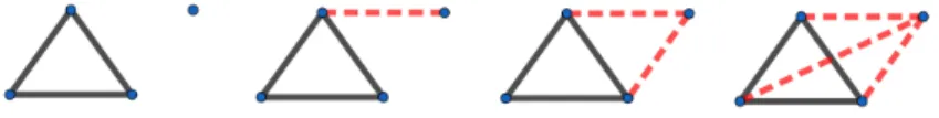
Here we describe the details of an evolution step. At every birth time 𝜏𝑖 a new vertex is added to the graph which can be connected to its ancestor triangle with𝑗 edges, where𝑗= 0,1,2,3. The vertices of the ancestor triangle to be connected to the new vertex are chosen uniformly at random. Let𝑝𝑗 denote the probability that
the new vertex will be connected to 𝑗 vertices of the ancestor triangle. It follows from the definition of the evolution process that at each birth step the possible number of the new triangles can be 0,1 or 3. On Figure 1 we represent these possibilities. The initial triangle is drawn by solid lines while the new ingredients by dashed lines. Denote the litter sizes belonging to the birth times 𝜏1, 𝜏2, . . . by
Figure 1: Possible birth events (0, 1, 2 or 3 new edges)
𝜀1, 𝜀2, . . .. Then𝜀1, 𝜀2, . . . are independent identically distributed discrete random variables with distribution P(𝜀𝑖=𝑗) =𝑞𝑗, 𝑗≥0. In our model the distribution of the litter size𝜀𝑖 is given by
P(𝜀𝑖= 0) =𝑞0=𝑝0+𝑝1, P(𝜀𝑖= 1) =𝑞1=𝑝2, P(𝜀𝑖= 3) =𝑞3=𝑝3, P(𝜀𝑖=𝑗) =𝑞𝑗= 0, if 𝑗 /∈ {0,1,3}.
We assume that the litter sizes are independent of the birth times 𝜏1, 𝜏2, . . ., too.
Denote by𝜆the life length of the generic triangle. 𝜆is a finite nonnegative random variable. After its death the triangle does not produce offspring, therefore 𝜉(𝑡) = 𝜉(𝜆)when𝑡 > 𝜆. Then the reproduction process of a triangle is
𝜉(𝑡) = ∑︁
𝜏𝑖≤𝑡∧𝜆
𝜀𝑖 =𝑆Π(𝑡∧𝜆),
where 𝑆𝑛 =𝜀1+· · ·+𝜀𝑛 gives the total number of offspring before the (𝑛+ 1)th birth event and𝑥∧𝑦 denotes the minimum of{𝑥, 𝑦}.
Let𝐿(𝑡)be the distribution function of𝜆. We assume that the survival function of the triangle’s life length is
1−𝐿(𝑡) =P(𝜆 > 𝑡) = exp
⎛
⎝−
∫︁𝑡 0
𝑙(𝑢) d𝑢
⎞
⎠,
where 𝑙(𝑡) is the hazard rate of the life span 𝜆. Moreover, we assume that the hazard rate depends on the number of offspring as
𝑙(𝑡) =𝑏+𝑐𝜉(𝑡) with positive constants𝑏and𝑐.
The whole evolution process is the following. The life and the reproduction pro- cess of the initial triangle is the same as that of the above described generic triangle.
When a child triangle is born, then it starts its own life and reproduction process which is also defined by the same way as its parent triangle. The same applies to
the grandchildren, etc. Therefore the evolution of the network is described by a continuous time branching process. We underline that the life and reproduction process of any triangle have the same distribution as those of the generic triangle, but the reproduction processes of different triangles are independent.
3. Theoretical results
Here we summarize the theoretical results of our paper [5].
Let 𝜇(𝑡) = E𝜉(𝑡) be the expectation of the number of offspring of a triangle up to time 𝑡. The total number of offspring of a triangle is 𝜉(∞). The expected offspring number of a triangle can be calculated as
𝜇(∞) =E𝜉(∞) = (𝑞1+ 3𝑞3)E(𝜆) =
(𝑞1+ 3𝑞3)1 𝑐
∫︁1 0
(1−𝑢)𝑏+1𝑐−𝑞0−1𝑒3𝑐𝑢(𝑞3𝑢2−3𝑞3𝑢+3(𝑞1+𝑞3))d𝑢.
The probability of extinction is1if𝜇(∞)≤1.
Theorem 3.1. If𝜇(∞)>1, then the probability of the extinction of the triangles is the smallest non-negative solution of equation
𝑞1+𝑞3(𝑦2+𝑦+ 1) 𝑐
∫︁1 0
(1−𝑢)1+𝑏𝑐−𝑞0−1𝑒(𝑞1𝑦+𝑞3𝑦
3
𝑐 𝑢−𝑞3𝑐𝑦3𝑢2+𝑞33𝑐𝑦3𝑢3)d𝑢= 1. (3.1)
Assume that𝜇(∞)>1, that is our branching process is supercritical. Then the Malthusian parameter𝛼is the only positive solution of equation∫︀∞
0 𝑒−𝛼𝑡𝜇(𝑑𝑡) = 1.
We can see that
𝑞1+ 3𝑞3−𝑏−1< 𝛼 < 𝑞1+ 3𝑞3−𝑏.
In our model the Malthusian parameter 𝛼satisfies the equation
1 = (𝑞1+ 3𝑞3) 𝑐
∫︁1 0
(1−𝑢)𝛼+(𝑏+1)𝑐 −𝑞𝑐0−1𝑒3𝑞1𝑢+𝑞3𝑢(𝑢
2−3𝑢+3)
3𝑐 d𝑢. (3.2)
Now we give the asymptotic behaviour of the number of triangles. Let us denote by 𝑍(𝑡)the number of triangles alive at time𝑡. Let𝛼be the Malthusian parameter.
Theorem 3.2. We have
𝑡→∞lim 𝑒−𝛼𝑡𝑍(𝑡) =𝑌∞𝑚∞
almost surely and in𝐿1, where the random variable𝑌∞is nonnegative, it is positive on the event of non-extinction, it has expectation1 and
𝑚∞= 1
(𝑞1+ 3𝑞3)2∫︀∞
0 𝑡𝑒−𝛼𝑡(1−𝐿(𝑡))𝑑𝑡.
Now we turn to the asymptotic behaviour of vertices and edges. Let us denote by𝑉(𝑡)the total number of vertices (dead or alive) up to time𝑡. Let𝑊(𝑡)be the number of edges (dead or alive) up to time 𝑡. Let 𝛾 denote the number of new edges at a birth. Then its distribution isP(𝛾=𝑗) =𝑝𝑗, 𝑗= 0,1,2,3.
Theorem 3.3. We have 𝑉(𝑡) 𝑍(𝑡) → 1
𝛼 and 𝑊(𝑡)
𝑍(𝑡) → E𝛾 𝛼 as𝑡→ ∞almost surely on the event of non-extinction.
4. Numerical and simulation results
To get a closer look on the theoretical results, we made some simulations about them. We generated our code in Julia language [4]. We chose Julia, because of the great implementation of priority queues. The simulation time of our code was significantly faster in Julia than in other programming languages. We handled the main objects (the triangles) of our model as arrays with 3 elements. The elements were the indices of the edges that formed an individual for the process. We put all triangles in a priority queue with the priority of its birth time, because we can pop out the element with the lowest priority. After we have got the triangle with the lowest birth time, we can handle its birth process with the predefined parameters 𝑏, 𝑐, 𝑞1, 𝑞3. In the birth process we generated an exponential time step for the next birth step of our triangle. After that we checked if the triangle is still alive by calculating the survival function. If the triangle is dead, we move to the next one.
If it is alive, then we generate 1 or 3 new triangles and put them into the priority queue with the calculated birth time priorities. After this step we moved to the next birth event. The pseudocode of the birth process is seen at Algorithm 1.
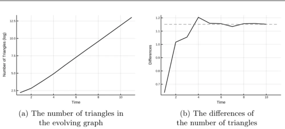
We made several simulation experiments. Here we show only some typical results. For the above demonstration first we used the parameter set 𝑏= 0.2, 𝑐= 0.2, 𝑝0 = 0.05, 𝑝1 = 0.05, 𝑝2 =𝑞1 = 0.6, 𝑝3 =𝑞3 = 0.3. On Figure 2a the solid curve shows the number of triangles. According to Theorem 3.2 it has asymptotic rate 𝑒𝛼𝑡. Therefore we put logarithmic scale on the vertical axis, so the function 𝑍(𝑡)is a straight line for large values of𝑡. On the figure one can see that the shape of the curve is close to a straight line, so it supports our Theorem 3.2.
Then we checked the value of the Malthusian parameter𝛼. We can find it in two ways. On the one hand, the slope of the line on Figure 2a is𝛼for large values of the time. This slope can be approximated by the differences of the function. So on Figure 2b we present these differences (solid line). On the other hand, 𝛼can be calculated numerically from equation (3.2). This𝛼value is shown of Figure 2b by the horizontal dashed line. The fit of the differences to this 𝛼can be seen for large values of 𝑡. To get a closer look on the Malthusian parameter 𝛼, we fixed 5 parameter sets. Then we calculated 𝛼 from equation (3.2) for each case. It is shown in the fifth column of Table 1. Then for each of the parameter sets we
2 4 6 8 10 2.5
5.0 7.5 10.0 12.5
Time
Number of Triangles (log)
(a) The number of triangles in the evolving graph
2 4 6 8 10
0.7 0.8 0.9 1.0 1.1 1.2
Time
Differences
(b) The differences of the number of triangles Figure 2: Simulation results for𝑏= 0.2, 𝑐= 0.2, 𝑞1= 0.6, 𝑞3= 0.3
simulated our process𝑍(𝑡)five times. Then we calculated the differences oflog𝑍(𝑡) which should be good approximations of 𝛼according to Theorem 3.2. In Table 1,
̂︁
𝛼1, 𝛼̂︁2, ̂︁𝛼3, 𝛼̂︁4, 𝛼̂︁5 show the values of these approximations for large𝑡. One can see that each 𝛼̂︀𝑖 is close to the corresponding𝛼. We calculated numerically the
𝑏 𝑐 𝑞1 𝑞3 𝛼 ̂︁𝛼1 ̂︁𝛼2 ̂︁𝛼3 ̂︁𝛼4 ̂︁𝛼5
0.2 0.4 0.7 0.1 0.5628 0.5651 0.5730 0.5701 0.5611 0.5594 0.2 0.4 0.8 0.1 0.6531 0.6537 0.6497 0.6570 0.6510 0.6589 0.4 0.4 0.8 0.1 0.4531 0.4503 0.4519 0.4584 0.4541 0.4524 0.4 0.4 0.7 0.2 0.6545 0.6533 0.6517 0.6548 0.6534 0.6574 0.4 0.4 0.6 0.3 0.8535 0.8519 0.8489 0.8559 0.8547 0.8566
Table 1: 𝛼from equation (3.2) and𝛼̂︀𝑖from simulations
probability of extinction from equation (3.1). It is shown in the column ‘Numerical’
of Table 2. In the column ‘Simulation’ the relative frequency of the extinction is shown using our computer experiment. For each parameter sets, we simulated 104 processes and counted the number of extinctions occured. The value of the relative frequency is close to the corresponding value of the probability in each case. So Table 2 supports the result of Theorem 3.1. To investigate how our difference process approximates 𝛼for large values of time𝑡, we simulated around 500 independent processes with the same parameters 𝑏 = 0.2, 𝑐 = 0.2, 𝑝0 = 0.05, 𝑝1 = 0.05, 𝑝2 = 𝑞1 = 0.6, 𝑝3 = 𝑞3 = 0.3 and same running time. Then we checked the differences of the last two values in the numbers of triangles that we simulated and made a histogram, seen in Figure 3. From equation (3.2) we obtained that the value of𝛼is0.3365. We see that the values of the differences are in [0.332,0.340], so they are very close to0.3365.
𝑏 𝑐 𝑞1 𝑞3 Simulation Numerical
0.0 0.2 0.4 0.4 0.0 0.0
0.1 0.2 0.4 0.4 0.1304 0.1282
0.1 0.2 0.5 0.4 0.1165 0.1158
0.1 0.2 0.5 0.5 0.1097 0.1025
0.2 0.2 0.5 0.4 0.2227 0.2180
0.2 0.2 0.6 0.4 0.2038 0.2002
0.3 0.3 0.5 0.4 0.3231 0.3185
0.4 0.4 0.5 0.4 0.3966 0.4020
Table 2: The relative frequency and the probability of the extinction of the triangles
Figure 3: Histogram of differences
To get some information about the random variable𝑌∞𝑚∞ represented in Theo- rem 3.2, we calculated the value of𝑍(𝑡)𝑒−𝛼𝑡 for103 independent repetitions of the process for the same time𝑡and same parameters 𝑞1= 0.3, 𝑞3= 0.6, 𝑏= 0.2, 𝑐= 0.2. On Figure 4 we represent the histogram and the empirical cumulative dis- tribution function (ECDF) calculated from the simulation. We obtained that the empirical cumulative distribution function of𝑌∞𝑚∞ fits to a gamma distribution, as the Kolmogorov–Smirnov test gave us𝑝value 0.6713.
0 5 10 15 20
0.0 0.2 0.4 0.6 0.8
(a) Histogram of𝑍(𝑡)𝑒−𝛼𝑡
0 5 10 15 20
0.00 0.25 0.50 0.75 1.00
(b) ECDF of𝑍(𝑡)𝑒−𝛼𝑡 Figure 4: Simulation results for𝑍(𝑡)𝑒−𝛼𝑡
5. Summary
In this paper and in [5] we offer a network evolution model which describes col- laborations of 3 persons. Our model grasps certain features of real collaborations as emerging and disappearing collaborations, moreover collaborations of 2 persons are also allowed. Our numerical results confirm the theoretical ones. The present results prepare our future research on more complicated collaborations.
Algorithm 1 Birth process of a triangle
1: procedureBirth process
2: 𝑌 ←non-emptyPriority Queue
3: 𝑏, 𝑐, 𝑞1, 𝑞3←parameters of the survival function
4: 𝑥←dequeueY
5: if 𝑥is a new trianglethen
6: 𝑡0←the birth time of𝑥in the whole process
7: 𝑡←0, lifetime of𝑥
8: 𝑙←1, life variable
9: while𝑙= 1do
10: 𝑡←𝑡+𝐸𝑥𝑝(1)
11: 𝑝←the calculated survival function
12: if 𝑝 > 𝑈 𝑛𝑖(0,1)then
13: 𝑝0←𝑈 𝑛𝑖(0,1)
14: if 𝑝0< 𝑞1 then
15: take a new triangle with𝑡0+𝑡birth time to𝑌
16: offspring number is1at birth time𝑡
17: else if 𝑝0>1−𝑞3 then
18: take three new triangles with𝑡0+𝑡birth times to𝑌
19: offspring number is3at birth time𝑡
20: else
21: 𝑙←0
22: take 𝑡as the death time of𝑥to𝑌
References
[1] Á. Backhausz,T. F. Móri:A random graph model based on 3-interactions, Ann. Univ. Sci.
Budapest 36 (2012), pp. 41–52.
[2] A.-L. Barabási:Network science, Cambridge: Cambridge University Press, 2018.
[3] A.-L. Barabási,R. Albert:Emergence of scaling in random networks, Science 286.5439 (1999), pp. 509–512,
doi:https://doi.org/10.1126/fscience.286.5439.509.
[4] J. Bezanson,A. Edelman,S. Karpinski,V. B. Shah:Julia: A Fresh Approach to Nu- merical Computing, 2014, arXiv:1411.1607 [cs.MS].
[5] I. Fazekas,A. Barta,C. Nószály,B. Porvázsnyik:A continuous time evolution model describing 3-interactions, in: Manuscript, Debrecen, Hungary, 2020.
[6] R. van der Hofstad:Random Graphs and Complex Networks Vol. 1.Cambridge: Cambridge Series in Statistical and Probabilistic Mathematics, 2017,
doi:https://doi.org/10.1017/9781316779422.
[7] T. F. Móri,R. Sándor:A random graph model driven by timedependent branching dynam- ics, Ann. Univ. Sci. Budapest, Sect. Comp. 46.3 (2017), pp. 191–213.
[8] O. Nerman:On the convergence of supercritical general (C-M-J) branching processes, Z.
Wahrscheinlichkeitstheorie verw Gebiete 57 (1981), pp. 365–395, doi:https://doi.org/10.1007/BF00534830.
[9] S. Rosengren:A Multi-type Preferential Attachment Tree, Internet Math. 2018 (2018).