Numerical results on noisy blown-up matrices ∗
István Fazekas, Sándor Pecsora
University of Debrecen, Faculty of Informatics fazekas.istvan@inf.unideb.hu pecsora.sandor@inf.unideb.hu
Submitted: February 4, 2020 Accepted: July 1, 2020 Published online: July 23, 2020
Abstract
We study the eigenvalues of large perturbed matrices. We consider an Hermitian pattern matrix𝑃 of rank𝑘. We blow up𝑃 to get a large block- matrix𝐵𝑛. Then we generate a random noise 𝑊𝑛 and add it to the blown up matrix to obtain the perturbed matrix 𝐴𝑛 = 𝐵𝑛+𝑊𝑛. Our aim is to find the eigenvalues of𝐵𝑛. We obtain that under certain conditions𝐴𝑛has 𝑘‘large’ eigenvalues which are called structural eigenvalues. These structural eigenvalues of𝐴𝑛 approximate the non-zero eigenvalues of𝐵𝑛. We study a graphical method to distinguish the structural and the non-structural eigen- values. We obtain similar results for the singular values of non-symmetric matrices.
Keywords:Eigenvalue, symmetric matrix, blown-up matrix, random matrix, perturbation of a matrix, singular value
MSC:15A18, 15A52
1. Introduction
Spectral theory of random matrices has a long history (see e.g. [1, 5–8] and the references therein). This theory is applied when the spectrum of noisy matrices is
∗This work was supported by the construction EFOP-3.6.3-VEKOP-16-2017-00002. The project was supported by the European Union, co-financed by the European Social Fund.
doi: 10.33039/ami.2020.07.001 https://ami.uni-eszterhazy.hu
17
considered. In [2] and [3] the eigenvalues and the singular values of large perturbed block matrices were studied. In [4] we extended the results of [2] and [3] and we suggested a graphical method to study the asymptotic behaviour of the eigenval- ues. In this paper we consider the following important question for the numerical behaviour of the eigenvalues. How large the blown-up matrix should be in order to show the asymptotic behaviour given in the mathematical theorems? We also study the influence of the signal to noise ratio for our results.
Thus we consider a fixed deterministic pattern matrix𝑃, we blow up𝑃to obtain a ‘large’ block-matrix𝐵𝑛, then we add a random noise matrix𝑊𝑛. We present limit theorems for the eigenvalues of𝐴𝑛=𝐵𝑛+𝑊𝑛 as𝑛→ ∞and show corresponding numerical results. We also consider a graphical method to distinguish the structural and the non-structural eigenvalues. This test is important, because in real-life only the perturbed matrix 𝐴𝑛 is observed, but we are interested in eigenvalues or the singular values of 𝐵𝑛 which are approximated by the above mentioned structural eigenvalues/singular values of𝐴𝑛.
In Section 2 we list some theoretical results of [4]. In Section 3 the numerical results are presented. We obtained that the asymptotic behaviour of the eigenvalues can be seen for relatively low values of𝑛, that is if the block sizes are at least50, then we can use our asymptotic results. We also study the influence of the signal/noise ratio on the gap between the structural and non-structural singular values. Our numerical results support our graphical test visualised by Figure 1.
2. Eigenvalues of perturbed symmetric matrices
In this section we study the perturbations of Hermitian (resp. symmetric) blown-up matrices. We would like to examine the eigenvalues of perturbed matrices.
We use the following notation:
• 𝑃 is a fixed complex Hermitian (in the real valued case symmetric) 𝑘×𝑘 pattern matrix of rank𝑟
• 𝑝𝑖𝑗 is the(𝑖, 𝑗)’th entry of𝑃
• 𝑛1, . . . , 𝑛𝑘 are positive integers,𝑛=∑︀𝑘 𝑖=1𝑛𝑖
• 𝐵˜𝑛 is an𝑛×𝑛matrix consisting of𝑘2blocks, its block(𝑖, 𝑗)is of size𝑛𝑖×𝑛𝑗
and all elements in that block are equal to𝑝𝑖𝑗
• 𝐵𝑛 is called a blown-up matrix if it can be obtained from𝐵˜𝑛 by rearranging its rows and columns using the same permutation
Following [2], we shall use the growth rate condition
𝑛→ ∞ so that 𝑛𝑖/𝑛≥𝑐 for all 𝑖, (2.1) where 𝑐 > 0 is a fixed constant. Here we list those theorems of [4] which will be tested by numerical methods.
Proposition 2.1. Let 𝑃 be a symmetric pattern matrix, that is a fixed complex Hermitian (in the real valued case symmetric) 𝑘×𝑘 matrix of rank 𝑟. Let 𝐵𝑛 be the blown-up matrix of𝑃. Then𝐵𝑛 has𝑟non-zero eigenvalues. If condition (2.1) is satisfied, then the non-zero eigenvalues of𝐵𝑛 are of order𝑛 in absolute value.
Now, we assume that 𝑟𝑎𝑛𝑘(𝑃) = 𝑘. We shall consider the eigenvalues in de- scending order, so we have|𝜆1(𝐵𝑛)| ≥ · · · ≥ |𝜆𝑛(𝐵𝑛)|. Since 𝑘eigenvalues of 𝐵𝑛
are non-zero and the remaining ones are equal to zero, we shall call the first 𝑘 ones structural eigenvalues of 𝐵𝑛. Similarly, we shall call structural eigenvalue that eigenvalue of 𝐴𝑛, which corresponds to a structural eigenvalue of 𝐵𝑛. This correspondence will be described by Theorem 2.2 and Corollary 2.3. We shall see that the magnitude of any structural eigenvalue is large and it is small for the other eigenvalues.
First we consider perturbations by Wigner matrices. Next theorem is a gener- alization of Theorem 2.3 of [2] where the real valued case and uniformly bounded perturbations were considered.
Theorem 2.2. Let𝐵𝑛,𝑛= 1,2, . . ., be a sequence of complex Hermitian matrices.
Let the Wigner matrices 𝑊𝑛, 𝑛 = 1,2, . . ., be complex Hermitian 𝑛×𝑛 random matrices satisfying the following assumptions. Let the diagonal elements 𝑤𝑖𝑖 of 𝑊𝑛 be i.i.d. (independent and identically distributed) real, let the above diagonal elements be i.i.d. complex random variables and let all of these be independent. Let 𝑊𝑛 be Hermitian, that is𝑤𝑖𝑗 = ¯𝑤𝑗𝑖for all𝑖, 𝑗. Assume thatE𝑤112 <∞,E𝑤12= 0, E|𝑤12−E𝑤12|2=𝜎2 is finite and positive, E|𝑤12|4<∞. Then
lim sup
𝑛→∞
|𝜆𝑖(𝐵𝑛+𝑊𝑛)−𝜆𝑖(𝐵𝑛)|
√𝑛 ≤2𝜎
for all 𝑖almost surely.
Corollary 2.3. Let 𝐵𝑛, 𝑛= 1,2, . . ., be blown-up matrices of a complex Hermi- tian matrix 𝑃 having rank 𝑘. Assume that condition (2.1) is satisfied. Let the Wigner matrices 𝑊𝑛, 𝑛 = 1,2, . . ., satisfy the conditions of Theorem 2.2. Then Theorem 2.2 and Proposition 2.1 imply that𝐵𝑛+𝑊𝑛 has𝑘eigenvalues of order 𝑛 and the remaining eigenvalues are of order√𝑛almost surely.
So the structural eigenvalues have magnitude𝑛while the non-structural eigen- values have magnitude√𝑛.
3. Singular values of perturbed matrices
In this section we study the perturbations of arbitrary blown-up matrices. We are interested in the singular values of matrices perturbed by certain random matrices.
We use the following notation:
• 𝑃 is a fixed complex 𝑎×𝑏pattern matrix of rank 𝑟
• 𝑝𝑖𝑗 is the(𝑖, 𝑗)’th entry of𝑃
• 𝑚1, . . . , 𝑚𝑎 are positive integers,𝑚=∑︀𝑎 𝑖=1𝑚𝑖
• 𝑛1, . . . , 𝑛𝑏 are positive integers,𝑛=∑︀𝑏 𝑖=1𝑛𝑖
• 𝐵˜𝑛 is an 𝑚×𝑛 matrix consisting of 𝑎×𝑏 blocks, its block (𝑖, 𝑗) is of size 𝑚𝑖×𝑛𝑗 and all elements in that block are equal to𝑝𝑖𝑗
• 𝐵𝑛 is called blown-up matrix if it can be obtained from𝐵˜ by rearranging its rows and columns
Following [3], we shall use the growth rate condition
𝑚, 𝑛→ ∞ so that 𝑚𝑖/𝑚≥𝑐 and𝑛𝑖/𝑛≥𝑑 for all 𝑖, (3.1) where 𝑐, 𝑑 > 0 are fixed constants. The following proposition is an extension of Proposition 6 of [3] to the complex valued case.
Proposition 3.1. Let 𝑃 be a fixed complex 𝑎×𝑏 matrix of rank 𝑟. Let 𝐵 be the 𝑚×𝑛 blown-up matrix of𝑃. If condition (3.1)is satisfied, then the non-zero singular values of 𝐵 are of order √𝑚𝑛.
Now we consider perturbation with matrices having independent and identically distributed (i.i.d.) complex entries. Let 𝑥𝑗𝑘, 𝑗, 𝑘 = 1,2, . . ., be an infinite array of i.i.d. complex valued random variables with mean 0and variance 𝜎2. Let𝑋 = (𝑥𝑗𝑘)𝑚,𝑗=1, 𝑘=1𝑛 be the left upper block of size𝑚×𝑛.
Theorem 3.2. For each𝑚and𝑛let𝐵 =𝐵𝑚𝑛 be a complex matrix of size𝑚×𝑛 and let 𝑋 =𝑋𝑚𝑛 be the above complex valued random matrix of size 𝑚×𝑛with i.i.d. entries. Moreover, assume that the entries of𝑋 have finite fourth moments.
Assume that 𝑚, 𝑛→ ∞so that 𝐾1≤ 𝑚𝑛 ≤𝐾2, where0< 𝐾1≤𝐾2<∞are fixed constants. Denote by 𝑠𝑖 and 𝑧𝑖 the singular values of 𝐵 and𝐵+𝑋, respectively, 𝑠1≥ · · · ≥𝑠min{𝑚,𝑛},𝑧1≥ · · · ≥𝑧min{𝑚,𝑛}. Then for all 𝑖
|𝑠𝑖−𝑧𝑖|= O(√ 𝑛) as𝑚, 𝑛→ ∞ almost surely.
Corollary 3.3. Proposition 3.1 and Theorem 3.2 imply the following. Let 𝑃 be a fixed complex 𝑎×𝑏 matrix of rank 𝑟. Let 𝐵 be the 𝑚×𝑛 blown-up matrix of 𝑃. Assume that condition (3.1)is satisfied. Let𝑋 be complex valued perturbation matrices satisfying the assumptions of Theorem 3.2. Denote by 𝑧𝑖 the singular values of 𝐵+𝑋, 𝑧1 ≥ · · · ≥ 𝑧min{𝑚,𝑛}. Then 𝑧𝑖 are of order 𝑛 for 𝑖 = 1, . . . , 𝑟 and 𝑧𝑖 = O(√𝑛) for𝑖=𝑟+ 1, . . . ,min{𝑚, 𝑛} almost surely as 𝑚, 𝑛→ ∞ so that 𝐾1≤𝑚𝑛 ≤𝐾2, where0< 𝐾1≤𝐾2<∞are fixed constants.
So the structural singular values (i.e. the largest 𝑟values) are ‘large’, and the remaining ones are ‘small’.
4. Numerical results
4.1. Eigenvalues of a symmetric matrix perturbed with Wigner noise
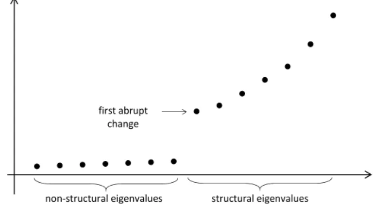
In [4] we concluded the following facts. In the case when the perturbation matrix has zero mean random entries, then the structural eigenvalues are ‘large’ and the non-structural ones are ‘small’. More precisely let|𝜆1| ≥ |𝜆2| ≥. . . be the absolute values of the eigenvalues of the perturbed blown-up matrix in descending order.
Then the structural eigenvalues|𝜆1| ≥ |𝜆2| ≥ · · · ≥ |𝜆𝑙|are ‘large’ and they rapidly decrease. The other eigenvalues|𝜆𝑙+1| ≥ |𝜆𝑙+2| ≥. . . are relatively small and they decrease very slowly. To obtain the structural eigenvalues we can use the following numerical (graphical) procedure. Calculate some eigenvalues of 𝐴𝑛 starting with the largest ones in absolute value. Stop when the last 5-10 eigenvalues are close to zero and they are almost the same in absolute value. Then we obtain the increasing sequence|𝜆𝑡| ≤ |𝜆𝑡−1| ≤ · · · ≤ |𝜆1|. Plot their values in the above order, then find the first abrupt change. If, say,
0≈ |𝜆𝑡| ≈ |𝜆𝑡−1| ≈ · · · ≈ |𝜆𝑙+1| ≪ |𝜆𝑙|<· · ·<|𝜆1|,
that is the first abrupt change is at 𝑙, then𝜆𝑙, 𝜆𝑙−1, . . . , 𝜆1 can be considered as the structural eigenvalues. The typical abrupt change after the non-structural eigenvalues can be seen in Figure 1.
non-structural eigenvalues structural eigenvalues first abrupt
change
Figure 1: The abrupt change after the non-structural eigenvalues
Our first example supports Theorem 2.2 and Corollary 2.3 in the real valued case. The following results were obtained using the Julia programming language version 1.1.1. The simulations were divided into four steps. Let 𝑃 be the real
symmetric pattern matrix
⎡
⎢⎢
⎢⎢
⎢⎢
⎢⎢
⎢⎢
⎢⎢
⎢⎢
⎢⎢
⎢⎣
8 7 2 5 3 2 4 0 3 1 7 9 6 3 4 0 2 5 2 0 2 6 7 6 5 4 2 0 3 4 5 3 6 8 7 6 0 5 4 2 3 4 5 7 9 8 8 6 5 1 2 0 4 6 8 7 6 8 0 4 4 2 2 0 8 6 9 7 6 6 0 5 0 5 6 8 7 8 8 4 3 2 3 4 5 0 6 8 9 6 1 0 4 2 1 4 6 4 6 5
⎤
⎥⎥
⎥⎥
⎥⎥
⎥⎥
⎥⎥
⎥⎥
⎥⎥
⎥⎥
⎥⎦ .
In the initial step we have matrix𝑃. It has the following eigenvalues: 45.302, 15.497,10.914,7.677,−7.245,6.188,4.696,−3.789,−3.381and3.141. This matrix is blown up with the help of a vector containing the size informations of the blocks.
If the vector is n= [𝑛1, 𝑛2, . . . , 𝑛10], then the first row of blocks is built with the following block sizes: 𝑛1×𝑛1, 𝑛1×𝑛2, . . .𝑛1×𝑛10, the second row of blocks:
𝑛2×𝑛1, 𝑛2×𝑛2, . . .𝑛2×𝑛10 and we continue this pattern till the last row. In different simulations we used different vectorsnto blow up the matrix, it will be detailed separately for each simulation.
The next step is to generate the noise matrix, which is a symmetric real Wigner matrix, as defined in Section 2. The entries are generated in the following way: let the diagonal elements 𝑤𝑖𝑖 of 𝑊𝑛 be i.i.d. real with standard normal distribution, let the above diagonal elements be i.i.d. real random variables and let all of these be independent. The size of the noise matrix is equal to the size of the blown up matrix. After that, in order to obtain the noisy matrix, in each iteration we generate a new Wigner matrix and add to the blown up matrix.
As the last step we calculate the eigenvalues of the perturbed matrix. To do so we used theeigvalsfunction from theLinearAlgebrapackage. Julia provides native implementations of many common and useful linear algebra operations which can be loaded withusing LinearAlgebra, to install the package we usedusing Pkg and then with thePkg.add("LinearAlgebra")command we installed the package.
We studied 4 different schemes to blow up matrix𝑃, in each of these 4 schemes we applied 6 different block size vectors. These block series are given in Table 1.
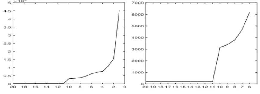
We realised 1000 simulations for all block series in Table 1 and checked if the abrupt change like in Figure 1 was seen. For very low values of𝑛𝑖we did not find the abrupt change. In each case the first well distinguishable abrupt change appeared when𝑛1 was 50. This result is shown in Figures 2, 3, 4, and 5. At each figure the left side: |𝜆20(𝐴𝑛)| <· · · <|𝜆1(𝐴𝑛)|; right side: |𝜆20(𝐴𝑛)|<· · · <|𝜆6(𝐴𝑛)| in a typical realization in our example. The right side figures show only a part of the sequence around the change, so the jumps are clearly seen.
Each of the figures shows that there is an abrupt change between the11th and 10theigenvalues. So we can decide that the 10 largest eigenvalues are the structural
ones (which is the true value, since we used matrix𝑃 having rank 10).
Name of the scheme Series of the blocks
Equal
𝑛1=𝑛2=· · ·=𝑛10= 10 𝑛1=𝑛2=· · ·=𝑛10= 20 𝑛1=𝑛2=· · ·=𝑛10= 50 𝑛1=𝑛2=· · ·=𝑛10= 100 𝑛1=𝑛2=· · ·=𝑛10= 500 𝑛1=𝑛2=· · ·=𝑛10= 1000
Two types
𝑛1=𝑛2=· · ·=𝑛5= 10, 𝑛6=· · ·=𝑛10= 20 𝑛1=𝑛2=· · ·=𝑛5= 20, 𝑛6=· · ·=𝑛10= 40 𝑛1=𝑛2=· · ·=𝑛5= 50, 𝑛6=· · ·=𝑛10= 100 𝑛1=𝑛2=· · ·=𝑛5= 100, 𝑛6=· · ·=𝑛10= 200 𝑛1=𝑛2=· · ·=𝑛5= 500, 𝑛6=· · ·=𝑛10= 1000 𝑛1=𝑛2=· · ·=𝑛5= 1000, 𝑛6=· · ·=𝑛10= 2000
Arithmetic progression
𝑛1= 10, 𝑛2= 20, . . . , 𝑛10= 100 𝑛1= 20, 𝑛2= 30, . . . , 𝑛10= 110 𝑛1= 50, 𝑛2= 60, . . . , 𝑛10= 140 𝑛1= 100, 𝑛2= 110, . . . , 𝑛10= 190 𝑛1= 500, 𝑛2= 510, . . . , 𝑛10= 590 𝑛1= 1000, 𝑛2= 1010, . . . , 𝑛10= 1090
Four types
𝑛1=𝑛2= 10, 𝑛3=𝑛4=𝑛5= 20, 𝑛6=𝑛7=𝑛8= 30, 𝑛9=𝑛10= 40 𝑛1=𝑛2= 20, 𝑛3=𝑛4=𝑛5= 40, 𝑛6=𝑛7=𝑛8= 60, 𝑛9=𝑛10= 80 𝑛1=𝑛2= 50, 𝑛3=𝑛4=𝑛5= 100, 𝑛6=𝑛7=𝑛8= 150, 𝑛9=𝑛10= 200 𝑛1=𝑛2= 100, 𝑛3=𝑛4=𝑛5= 200, 𝑛6=𝑛7=𝑛8= 300, 𝑛9=𝑛10= 400 𝑛1=𝑛2= 500, 𝑛3=𝑛4=𝑛5= 1000, 𝑛6=𝑛7=𝑛8= 1500, 𝑛9=𝑛10= 2000 𝑛1=𝑛2= 1000, 𝑛3=𝑛4=𝑛5= 2000, 𝑛6=𝑛7=𝑛8= 3000, 𝑛9=𝑛10= 4000 Table 1: Schemes used to blow up matrix𝑃
0 2 4 6 8 10 12 14 16 18 20 0 500 1000 1500 2000 2500
6 7 8 9 10 11 12 13 14 15 16 17 18 19 20 0 50 100 150 200 250 300 350
Figure 2: Equal: 𝑛1=𝑛2=· · ·=𝑛10= 50
0 2 4 6 8 10 12 14 16 18 20 0 500 1000 1500 2000 2500 3000 3500 4000
6 7 8 9 10 11 12 13 14 15 16 17 18 19 20 0 50 100 150 200 250 300 350 400 450 500 550
Figure 3: Two types: 𝑛1=· · ·=𝑛5= 50,𝑛6=· · ·=𝑛10= 100
0 2 4 6 8 10 12 14 16 18 20 0 500 1000 1500 2000 2500 3000 3500 4000 4500 5000
6 7 8 9 10 11 12 13 14 15 16 17 18 19 20 0 100 200 300 400 500 600 700
Figure 4: Arithmetic progression: 𝑛1= 50, 𝑛2= 60, . . . , 𝑛10= 140
0 2 4 6 8 10 12 14 16 18 20 0 1000 2000 3000 4000 5000 6000 7000
6 7 8 9 10 11 12 13 14 15 16 17 18 19 20 0 100 200 300 400 500 600 700 800
Figure 5: Four types: 𝑛1=𝑛2= 50, 𝑛3=𝑛4=𝑛5= 100, 𝑛6=𝑛7=𝑛8= 150, 𝑛9=𝑛10= 200
As the block’s sizes are increasing, the border between the structural and non- structural eigenvalues is getting more and more significant, as it is shown in Fig- ure 6. We see, that when𝑛𝑖 = 1000(for all𝑖), then the gap is much larger than in the case of 𝑛𝑖= 50.
0 2 4 6 8 10 12 14 16 18 20 0 0.5 1 1.5 2 2.5 3 3.5 4 4.5
5 104
6 7 8 9 10 11 12 13 14 15 16 17 18 19 20 0 1000 2000 3000 4000 5000 6000 7000
Figure 6: Equal: 𝑛1=𝑛2=· · ·=𝑛10= 1000
In Table 2, we list the averages of the absolute values of the eigenvalues making 1000 repetitions in each case. More precisely,𝑛𝑖means that all blocks were𝑛𝑖×𝑛𝑖
and in the column below𝑛𝑖 there are the 20 largest of the averages of the absolute values of the corresponding eigenvalues of different 𝐴𝑛 matrices. We see, that there is a gap between the10th and 11th values even in the relatively small value of 𝑛𝑖 = 10. The larger the value of 𝑛𝑖, the larger the gap. This table shows that our test is very reliable for moderate (e.g. 𝑛𝑖= 50) sizes of the blocks.
𝑗 𝑛𝑖= 10 𝑛𝑖= 20 𝑛𝑖= 50 𝑛𝑖= 100 𝑛𝑖= 200 𝑛𝑖= 500 𝑛𝑖= 1000 1 453.26 906.28 2265.40 4530.50 9060.70 22652.00 45303.00 2 155.64 310.65 775.43 1550.31 3100.00 7748.90 15497.00 3 110.06 219.28 546.65 1092.40 2183.90 5458.00 10915.00 4 77.99 154.82 385.08 768.93 1536.70 3839.60 7677.90 5 73.76 146.21 363.63 725.90 1450.40 3624.10 7246.90 6 63.36 125.32 310.93 620.41 1239.20 3095.40 6189.40
7 48.86 95.95 236.92 471.66 941.21 2349.90 4697.80
8 40.51 78.39 192.04 381.54 760.54 1897.10 3791.70
9 36.30 70.32 171.90 340.95 678.98 1693.20 3383.40
10 34.06 65.84 160.18 317.23 631.47 1573.90 3144.70
11 18.56 27.21 44.03 62.73 89.04 141.14 199.78
12 17.96 26.70 43.58 62.33 88.67 140.84 199.50
13 17.45 26.27 43.20 61.99 88.37 140.58 199.27
14 17.03 25.92 42.90 61.72 88.14 140.38 199.09
15 16.65 25.59 42.62 61.47 87.92 140.18 198.92
16 16.33 25.28 42.36 61.25 87.72 140.01 198.77
17 15.99 25.00 42.11 61.03 87.53 139.85 198.63
18 15.69 24.74 41.89 60.83 87.34 139.69 198.49
19 15.40 24.47 41.67 60.64 87.17 139.54 198.36
20 15.12 24.23 41.47 60.45 87.01 139.40 198.23
Table 2: Eigenvalues in the case of equal size blocks
4.2. Singular values of a non-symmetric perturbed matrix
This example supports Theorem 3.2 and Corollary 3.3. Let 𝑃 be the 7×8 real non-symmetric pattern matrix
⎡
⎢⎢
⎢⎢
⎢⎢
⎢⎢
⎣
6 5 6 5 3 2 1 2 3 9 6 7 4 5 6 1 4 8 9 8 3 4 2 1 5 7 6 8 7 5 3 2 2 5 7 8 9 6 5 3 1 3 4 5 6 7 6 4 2 1 4 6 7 8 9 9
⎤
⎥⎥
⎥⎥
⎥⎥
⎥⎥
⎦ .
In the previous example we showed the effect of the blocks’ sizes, now we show the effect of the signal to noise ratio (snr) on the singular values of 𝑃. To blow up 𝑃, we chose block heights as [𝑚1, . . . , 𝑚𝑎] = [500,750,500,600,750,550,500]
and block widths as[𝑛1, . . . , 𝑛𝑏] = [500,500,600,1000,550,500,550,500]. Then we blew up𝑃, and we added a noise to get the perturbed matrix. Like in Section 3, we denote by 𝐵 the blown-up matrix which is the signal, by 𝑋 the noise matrix, and by𝐴=𝐵+𝑋 the perturbed matrix. We shall use the following definition of the signal to noise ratio
snr=
1 𝑚𝑛
∑︀𝑚 𝑖=1
∑︀𝑛 𝑗=1𝑏2𝑖,𝑗
1 𝑚𝑛
∑︀𝑚 𝑖=1
∑︀𝑛 𝑗=1𝑥2𝑖,𝑗. Here 𝑚=∑︀𝑎
𝑖=1𝑚𝑖 is the number of rows, 𝑛=∑︀𝑏
𝑗=1𝑛𝑗 is the number of columns in 𝐵 and𝑋,𝑏𝑖,𝑗 is the element of the signal matrix𝐵, while𝑥𝑖,𝑗 is the element of the noise matrix𝑋 in the𝑖th row and𝑗th column.
In this example, the entries of the noise matrix𝑋 are independent and, at the initial step, they are from standard normal distribution. In each of the following steps we increased the noise, by multiplying each of the elements of the noise matrix by certain multipliers. The first multiplier was 1.002, the second one was1.004, then1.006, . . . ,3.000.
So, during the experiment, we amplify the noise step-by-step and check at each iteration the snr and the ratio of the last (smallest) structural singular value and the first (largest) non-structural one. If the structural/non-structural ratio reaches a certain point, the signal gets so noisy, that it is not possible any more to distinguish the structural singular values from the non-structural ones. On Figure 7 the dashed line is the signal to noise ratio and the solid line is the ratio of the the last (smallest) structural singular value and the first (largest) non-structural singular value. On the horizontal axis the scale is given by the variance of the noise. One can see, that when the noise grows, then the snr decreases quickly, but the structural/non-structural ratio decreases quite slowly. If the structural/non- structural ratio decreases close to 1, then we reach a point, where the structural and non-structural singular values are not well distinguishable any more. However, Figure 7 shows that our method is reliable, that is if the noise in not higher than
25%of the signal, then the structural singular values are well distinguishable from the non-structural ones.
1 6 11 16 21 26 31 36
1 2 3 4 5 6 7 8 9
snr Last structural singular value/First non-structural 3
Figure 7: Signal to noise ratio compared to structural/non-structural singular value ratio
5. Conclusion
The shown graphical method works appropriately to distinguish the structural and non-structural eigenvalues and singular values. The size of the blocks has an in- fluence on the ‘jump’ between the non-structural and the structural eigenvalues.
As the block’s sizes are increasing, the border between the structural and non- structural eigenvalues is getting more and more significant. If the block sizes are at least 50, then the structural and the non-structural eigenvalues are well distin- guishable. Our test is reliable, if the noise is less than 25%, but above this noise level it can be unreliable.
References
[1] Z. D. Bai:Methodologies in spectral analysis of large dimensional random matrices. A review.
Statistica Sinica 9 (1999), pp. 611–677.
[2] M. Bolla:Recognizing linear structure in noisy matrices.Linear Algebra and its Applications 402 (2005), pp. 228–244,
doi:https://doi.org/10.1016/j.laa.2004.12.023.
[3] M. Bolla,A. Krámli,K. Friedl:Singular value decomposition of large random matrices (for two-way classification of microarrays).J. Multivariate Analysis 101.2 (2010), pp. 434–
446,
doi:https://doi.org/10.1016/j.jmva.2009.09.006.
[4] I. Fazekas,S. Pecsora:On the spectrum of noisy blown-up matrices.Special Matrices 8.1 (2020), pp. 104–122,
doi:https://doi.org/10.1515/spma-2020-0010.
[5] Z. Füredi,J. Komlós:The eigenvalues of random symmetric matrices.Combinatorica 1 (1981), pp. 233–241,
doi:https://doi.org/10.1007/BF02579329.
[6] S. O’Rourke,D. Renfrew:Low rank perturbations of large elliptic random matrices.Elec- tron. J. Probab 19 (2014), pp. 1–65,
doi:https://doi.org/10.1214/EJP.v19-3057.
[7] T. Tao:Outliers in the spectrum of iid matrices with bounded rank perturbations.Probability Theory and Related Fields 155 (2013), pp. 231–263,
doi:https://doi.org/10.1007/s00440-011-0397-9.
[8] H. V. Van:Spectral norm of random matrices.Combinatorica 27 (2007), pp. 721–736, doi:https://doi.org/10.1007/s00493-007-2190-z.


![arXiv:2002.10324v2 [math.GT] 17 Apr 2020](data:image/gif;base64,R0lGODlhAQABAIAAAP///wAAACH5BAEAAAAALAAAAAABAAEAAAICRAEAOw==)