Performance analysis of MILP based model predictive control algorithms for dynamic railway scheduling
J´anos Rudan1, Bart Kersbergen2, Ton van den Boom2 and Katalin Hangos3
1Faculty of Information Technology, P´azm´any P´eter Catholic University
2Delft Center for Systems and Control, Delft University of Technology
3Computer and Automation Research Institute, Hungarian Academy of Sciences
E-mail: rudan.janos@itk.ppke.hu, b.kersbergen@tudelft.nl, a.j.j.vandenboom@tudelft.nl, hangos@sztaki.hu
Abstract— In this paper we analyse the performance of solvers for Mixed Integer Linear Programming (MILP) prob- lems that appear from the model predictive control of railway networks. Our aim is to study techniques that reduce the amount of delay using dynamic traffic management by the rescheduling of trains. Due to the size of the emerging MILP problem and the given constraints on solution time, a thorough analysis of different MILP solution techniques was necessary. It has been proven that a significant speedup in the solution time can be achieved by the proper restructuring of the matrices of the MILP problem. The simulation results also confirm the effectiveness of the proposed control technique and the ability of this setup to analyse the most delay-sensitive trains in the network.
I. INTRODUCTION
Considerable effort has been spent recently on the topic of delay management in a railway network via rescheduling trains. Delays can be caused by technical failures, accidents, weather conditions or other unexpected situations. Some of the delays can be handled by a stable and robust timetable [1] but in case of large delays, rerouting of the trains, reshuffling train orders or breaking connections can be necessary to minimize the effect of the disturbance.
Various quantitative models have been developed in the past mostly based on mathematical programming methods.
A comprehensive survey of these kinds of methods can be found in [2]. A delay-management problem handled as mixed- integer programming first appeared in [3] and more recently in [4]. In [5] a permutation-based methodology was proposed which uses max-plus algebra to derive a Mixed Integer Linear Programming (MILP) to find optimal rescheduling patterns [6].
In this paper the dynamic traffic management of railway networks is formulated as a Mixed Integer Linear Program- ming (MILP) problem [7] in a model predictive framework.
The network model is constructed in a way that the the order of the trains using the critical resource (namely the tracks) is con- trolled by binary variables. During the optimization this set of binary variables is determined while minimizing the given cost function. The solution of these kinds of problems can cause serious computational difficulties since integer programming is known to be NP-hard generally.
The proposed technique is capable of predicting a given network’s future behaviour in case of a cyclic timetable and find an optimal rescheduling of the trains to minimize the total delay in the network along the prediction horizon.
The structure of this paper is the following: in Section II the scheduling problem is introduced - namely the problem of dynamic traffic management of a railway network. In Section III the simulation results can be found while in Section IV the conclusions and possible future works are summarized.
II. FORMULATING THE MODEL
Consider a railway network having a periodic timetable with cycle timeT. In case ofnominal operationthe trains follow a pre-scheduled route repeated everyTminutes where the order of the trains on the tracks is naturally defined by the schedule.
The network can be deviated from the nominal operation by an emerging delay. We call the resulting schedule aperturbed mode. With every new schedule we can associate a perturbed mode.
A possible new schedule can be represented with a set of constraints determining the new order of the trains on the tracks. The aim of the control method is to find a set of con- straints which describes a schedule having minimal deviation from the nominal schedule.
In this section only a short review of the model will be discussed. More detailed explanation of the model can be found in [5], [8].
A. Modelling the trains and the tracks
The operation of the schedule can be divided into a set of train runs, where each run starts with a departure and ends with an arrival. A number of train runs, performed by the same
’physical’ train will be denoted as a line. In the remainder of this paper we will simply refer to a ’train run’ as a ’train’.
In this particular model we do not take into consideration the possible existence of parallel tracks between two stations which means that overtaking is possible only at stations. We also take the assumption that at the stations can host an unlimited number of trains and the order of departures from stations can be arbitrarily chosen.
B. Building up the constraint set
The departure and arrival times of the trains have to meet with the following constraints:
• Time schedule constraint: a departure may not occur before its scheduled departure time, so we have to satisfy the timetable constraint
di(k)≥rid(k) (1)
whererdi(k)is the scheduled departure time for the ith train in the kth cycle. For the arrival time a similar constraint can be expressed:
ai(k)≥rai(k) (2) This constraint forces the trains to have a nominal running running time which is usually greater than the minimal running time. If it is needed, the arrival constraints can be omitted by settingria(k)to−∞.
• Running time constraint:letti(k)be the minimum run- ning time of the ith train. The running time constraint then becomes
ai(k)≥di(k−δii) +ti(k) (3) whereδii = 0if the departure time and the arrival time are in the same cycle and δii = 1 if there is a cycle difference between departure and arrival.
• Dwell time constraint: let pi be the preceding train of trainion the same line, which means that trainiandpi are physically the same train. Letspi(k)be the minimum dwell time between arrival of trainpiand the departure of traini, then we have to satisfy the dwell time constraint
di(k)≥api(k−δipi) +spi(k) (4) whereδipi = 0if in cycle(k)trainpiarriving proceeds as trainiin the same cycle andδipi= 1otherwise.
• Headway constraints:letHi(k)be the set of trains that move over the same track and in the same direction as train i, and are scheduled before train iin the nominal operation mode. Letj ∈ Hi(k)and lethij denote the minimum headway time between trainjand traini. For each train j ∈ Hi(k)we have headway constraints for both departure and arrival
di(k)≥dj(k−δij) +hij+uij(k)β, ∀j∈ Hi(k) dj(k−δij)≥di(k) +hji+ (1−uij(k))β, ∀j∈ Hi(k)
(5) ai(k)≥aj(k−δij) +hij+uij(k)β,∀j∈ Hi(k) aj(k−δij)≥ai(k) +hij+ (1−uij(k))β,∀j ∈ Hi(k)
(6) whereβis a large negative number (soβ 0) anduij(k) is a binary variable with which we are able to control the values in the constraints, and through this, the order of the trains. Note that foruij(k) = 0, the constraints (5.a) and (6.a) will be active, and foruij(k) = 1, the constraints (5.b) and (6.b) will be active.
• Meeting constraints:letMi(k)be the set of trains that move over the same track and in the opposite direction as traini, and are scheduled before trainiin the nominal operation mode. Letj ∈ Mi(k)and letwij denote the minimum separation time between arrival of trainj and departure of traini. For each trainj ∈ Mi(k)we have separation constraint
di(k)≥aj(k−δij) +wij+uij(k)β, ∀j∈ Mi(k) dj(k−δij)≥ai(k) +wji+ (1−uij(k))β,∀j∈ Mi(k)
(7) where the role ofβanduij(k)is similar to the previous case.
Note that (1)-(7) describes the dynamical model of the system.
It should be noted that during nominal operation all δij values are equal to zero or one, but in perturbed operation other values are also possible. For sake of simplicity, we will consider only the case whenδij ={0,1}.
C. Model predictive control and MILP formulation A MILP problem can be stated as follows [7]:
minx cTx Ax≤b x≥0
xi∈Z, i= 1, . . . , ...nb
xj∈R, j=nb+ 1, . . . , nb+nr
(8)
wherenbis the number of integer (or binary) variables, and nr is the number of real state variables. Matrix A contains all the coefficients for the inequality constraints. It should be noted, that if they are present, reformulation of the equality constraints to inequality constraints is always possible [9]. We would like to reformulate the railway model, containing the above defined constraint set, as an MILP.
As it has been defined previously, let us consider a network havingntrain runs (or shortly trains), and define the following vectors:
z(k) =
di(k)
... dn(k) a1(k)
... an(k)
∈ R2n; r(k) =
r1d(k)
... rdn(k) r1a(k)
... ran(k)
∈R2n
(9) and the elementsui,j(k)withj∈ Hi(k)orj∈ Mi(k)can be stacked in one vectoru(k)∈Rm.
The goal of the model predictive controller is to minimize the sum of all delays, and so we come to the objective function (or performance index):
J(k) =
Np
X
j=0
Xn
i=1
σi
zi(k+j)−ri(k+j)
+
m
X
l=1
ρlul(k+j)
(10) Here Np is the prediction horizon, and σi, ρl are non- negative weighting scalars. The first term of Eq. 10 is related to the sum of all predicted departure and arrival delays, and the second term denotes the penalty for all train orders changes during cyclek+j. Note that due to constraints (1)-(2) there holdszi(k+j)−ri(k+j)≥0, ∀jand soJ(k)≥0.
Now define the extended vectors
˜ z(k) =
z(k) z(k+ 1)
... z(k+Np)
∈R2nNp
˜ u(k) =
u(k) u(k+ 1)
... u(k+Np)
∈RmNp
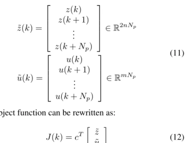
(11)
The object function can be rewritten as:
J(k) =cT z˜
˜ u
(12) whereccontains all the values σand ρ. Also the network constraints (1)-(7) can be written using the vectorsz˜ and u˜ and we obtain:
Az Au z(k)˜
˜ u(k)
≤b(k) (13) where matrix Az only consists of entries [Az]ij ∈ { −1,0,1}, matrix Au only consists of entries [Au]ij ∈ { −β ,0, β} and b(k) = b0 +b1z(k−1) +θ(k) where [b0]i ∈ {0, β}, [b1]i ∈ {0,1}, z(k −1) is the past value, andθ(k)is a vector with the schedule timesrd(k),ra(k), the minimum running timet(k), the minimum dwell timess(k), the minimum heading timesh(k), and the minimum separation timesw(k).
Considering (8), we have now recast the model predictive control problem into a MILP structure where the objective function is defined in (12) and the constraints in (13).
Note that the emerging optimization problem is always feasible by choosing a possibleu˜there will be always a proper
˜
zwhich satisfies the constraints.
III. SIMULATION RESULTS
Simulations were done using the model of the Dutch railway system (see Fig. 1), with a cycle time T = 60 min. The network model consists of 41 stations and 118 tracks. In the timetable only the international and interregional trains are included, the local trains are excluded. For the simulations Np = 2is selected, so the prediction is done for 2 hours in the future.
Fig. 1: The Dutch railway network.
The generated problem has 26712 constraints and 5316 variables from which 1728 are continuous variables (departure and arrival times) and the remaining 3588 are binary.
The simulations were completed on a personal computer having a 4-core Pentium IV CPU running on 3.4GHz.
Our aim was to solve the problems generated from the scenarios in less than120secon average, because in that case the software is able to track the changes in the railway network on-line.
A. Scenario generation
In order to simulate the perturbed operation of the system, a new parameter vectorθis generated containing all the devia- tions from values in the original schedule described byθ0. It is shown in [10] that the distribution of delays appearing in a train network follow a Weibull distribution. In our case delays were generated according to a Weibull-distribution having shape parameter0.8 and scale parameter5. Maximal delay was set to40minand the average introduced delay to10min.
A given percentage of the trains were selected from all the trains and the delay values were added to their departure and arrival data, according to two different scenarios:
• case 1: 8% of the trains were selected to be delayed.
• case 2: 20 % of the trains were selected to be delayed.
We usedcase 1in simulations during the selection of the solver (see Section III-B) and we usedcase 2in other tests.
The reader should note that according to the the infrastruc- ture manager company of the Dutch Railways, in the first nine months of 2012,10.5%of the trains in the Netherlands had 3 minutes or more delay. This means thatcase 2is related to a much more complex scenario than normal cases.
B. Selecting the proper MILP solver
There are several available MILP solvers both originating from the free software community and commercial ones [11].
Comparison of the solvers considering the used techniques and algorithms can be found in [12]. Another interesting and continuously maintained review of the solver’s performance can be found at [13].
State-of-art solvers implement strongly heuristic-driven branch-and-cut algorithms to solve MILP problems [14]. Be- cause of their crucial role in the solution speed, heuristics applied in MILP solvers are the subject of extensive research in the recent years [15], [16].
It should be emphasized that depending on the structure, size and other properties of the current MILP problem it is always a good idea to review the performance of the available solvers. According to the different algorithms applied by the solvers huge differences could appear both in quality and the time of the solution.
During the present work the following solvers were inves- tigated: from the COIN-OR [17] community: DIP (version 0.83.2), SYMPHONY (version 5.4.4), CBC (version 2.7.6).
Also GLPK (version 4.32) and CPLEX (version 12.1) were involved in the tests. The selection process was based on two criteria: on one hand the ability of parallel solution and on the other hand the average solution time.
Fig. 2: Comparison of solution times in case of different MILP problems. CBC outperforms all the other solvers. In the scenarios 8% of trains were selected randomly to be delayed.
The solvers were compared based on their average solution time processing a given problem set. The method of the prob- lem generation is detailed in Section III. DIP and GLPK were unable to solve any of the problems - neither problems with the original nor with the reordered structure - in the given maximal time limit (300sec). The results of the three remaining solvers can be seen in Figure 2. All solvers were set to run on single- thread mode (no parallelism).
Based on the results we concluded that CBC was the fastest solver and it produced the smallest variations in solution time while solving different scenarios. According to this we used CBC to complete all the other tests and simulations.
Note that the selection of the solver is always an arbitrary choice, there could be some other available solvers which we didn’t considered.
C. Track-based reordering of the constraint matrix
As it can be found in [14], the effectiveness of the al- gorithms applied during the solution of the MILP strongly depends on the structure of the A matrix. By investigating those methods, one can see that building up a constraint matrix having clear block-angular structure is the most beneficial.
Based on these, the constraint matrix has been reordered on a per-track basis. This means that we collect into one block all the constraints and control variables corresponding to a given track. Based on the timetable the track of each train run can be determined and based on this the order of the corresponding constraints can be completed.
It can be easily seen that the order of the trains on one track is independent of the order on another track. By reordering the constraint set on track-basis we can see similar structure in the MILP formulation. The different constraint blocks correspond- ing to a given track are independent from each other, and the blocks themselves are connected via the continuity constraints.
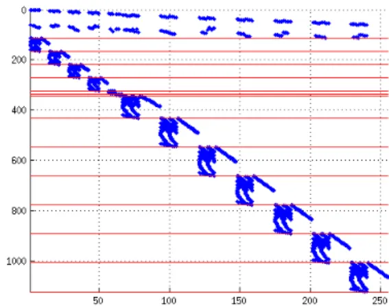
In Fig. 3. one can see the result of the track-based ordering approach. The formulated blocks can be seen clearly. It is clear that any other algorithm generating the constraint set could give some structure to the constraint matrix but, among the examined cases the track-based approach gives the best result. The increase in solution speed gained by the proposed reordering is detailed in Section III-D.
Fig. 3: Structure of the constraint matrix where the variables are on the x-axis and the equations are on the y-axis. As it can be seen, the result of the track-based ordering is a clear block-angular structure. To be able to see the details, a smaller size model was used containing1124 constraints and254variables.
D. Effect of reordering on the solution time
As was mentioned before, the effect of proper restructuring of the given MILP problem can have huge impact on the solution time. In the present work we selected a track-based ordering which leads to a clear block-angular structure. The following results verify that even in the presence of the solver’s preprocessor a serious gain can be achieved by a proper problem formulation.
In the tests we considered two cases. First the columns and rows of the formulated matrices were generated in a random order resulting an unordered matrix structure. In the other case we built up the matrices of the same problem with track-based ordering (see Sec. III-C).
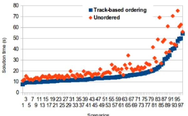
The solution times in both cases for several different sce- nario can be seen in Fig. 4. for several different scenarios. In the presented case the test set consists of 97 different scenarios.
The average solution time was 23,97 sec (s = 14,51 sec) without and17,11sec(s= 10,13sec) with reordering so the time gain obtained by the reordering was6.85secon average (s= 7.04sec) which means an average speedup ratio1,407.
Note that to minimize the problem-specific knowledge in the unordered case, we used only the built-in preprocessors of the MILP solver. Considering this, the results emphasize the importance of the structured problem formulation based on problem-specific knowledge.
E. Results in case of distributed solution
As it was discussed Section III-B. several available solvers offers the capability of parallel solution of MILP problems [18]. This approach could be quite advantageous in case of large-scale problems.
The simulation result using CBC shows the advantage of the distributed solution. In Fig. 5. the average solution time of a problem set having 100 elements can be seen in case of single- thread and multi-thread setups. Fig. 5. shows that the solution
Fig. 4: Solution times in case of a random constraint matrix structure or in case of the track-based reordering. The simulation results show that even in the presence of the preprocessor of the solver proper reordering can yield to significant speedup. Scenarios (in which 20% of trains were selected randomly to be delayed) are plotted in an increasing order w.r.t. the solution time in case of track-based ordering.
Fig. 5: Average elapsed time of solving a MILP with multiple threads on a 4-core computer. Using 4 threads gives the best result.
time scales well with the number of the involved CPU cores.
The maximal speedup can be achieved if the number of threads is equal to the number of physical cores in the processor.
F. Effectiveness of the proposed control technique
To measure the performance of the control technique, the following tests were completed. 176 scenarios were generated according to Section III-A and8%of the trains were selected to be delayed. Each scenario has different initial (primary) delays.
Using these scenarios we simulated the uncontrolled be- haviour of the network. During this open-loop simulation all control inputs were set to zero. At the end of the prediction horizon the difference between the result and the reference schedule is calculated as the sum of the delays. For the same scenario set we have done the simulation and the calculation of the sum of the delays in controlled mode, too.
The comparison of the sum of the delays shows the per- formance of the control techniques as can be seen in Fig. 6.
We found that the proposed technique can decrease the sum of the delays with30%compared to the uncontrolled case while averagely20control actions were applied.
It should be noted, that during these tests the solution of the problem is successfully found by the solver in less than the desired time limit (120sec).
Fig. 6: Effect of optimal reordering of the trains in case of delays. As it can be seen the sum of the delays in the network can be significantly reduced over the control horizon with the help of the proposed control technique. Scenarios (in which 20% of trains were selected randomly to be delayed) are plotted in an increasing order w.r.t. the total secondary delay in the network.
G. Analysis of delay sensitivity in the network
It is known that in a railway network the change of the departure or arrival time of one train can a have small effect, but the change of the parameters of other trains can lead to an immense effect on the whole system. In the following it is shown that the proposed model structure is capable of showing the most delay-sensitive parts of the network.
To investigate the effect of a given train’s delay on the network, the following setup was used. Two different cases were examined introducing5and10minutes of primary delay to a given train, respectively. The whole network model with Np = 2 was generated and simulated over the prediction horizon. Both uncontrolled case and controlled case were evaluated. This procedure was iterated over all trains in the network.
This setup enables us to analyse the effect of delay on a given train. If the selected train is a bottle-neck node in the network, then the introduced changes of its departure and arrival times results high secondary delay values in the network showing that many other trains are effected by the delay of this one.
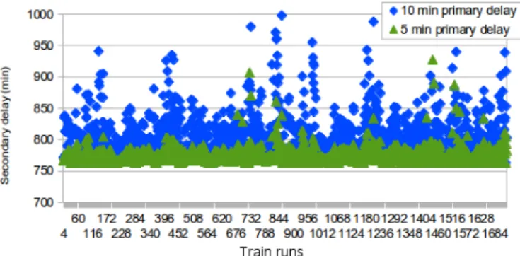
The generated results can be seen in Fig. 7 and in Fig. 8.
In case of the5minprimary delay, the average of secondary delay in uncontrolled mode is778.37min(s = 11.95min) while in controlled mode 413.96 min (s = 10.37min) is achieved. In case of 10 min primary delay, the average of the secondary delays is800.99 min (s = 39.65 min) and 430.49min(s= 27.08min) in uncontrolled and controlled case, respectively (where s stands for standard deviation).
These results also confirm that the proposed control technique can effectively reduce the amount of the delay in the network.
It should be noted that this algorithm works with the train runs in the model. As it is introduced in Section II-A a train run is a representation of a specific train over a given track.
Handling train runs brings the advantage that besides being able to analyse the delay-sensitivity of a train we can also determine the most delay-sensitive track in the train’s route.
Fig. 7: Result of delay-sensitivity tests in case of uncontrolled mode. Both the scenarios having5 and10minutes primary delay are represented.
Fig. 8: Result of delay-sensitivity tests in case of controlled mode. Both the scenarios having5 and10minutes primary delay are represented. Delay values are clearly smaller than in Fig. 7.
IV. CONCLUSIONS AND FUTURE WORK
In this paper the performance of a railway management technique [8] has been analysed. The rescheduling problem in a railway network is recast as a MILP problem and solved in an MPC architecture. Due to the computational complexity of the emerging MILP problem and the time constraints on the solution it was necessary to speed up the solution with proper handling of the original problem.
The main contributions of the present work are the follow- ing: using a track-based ordering a significant speedup can be achieved during the solution process. The most efficient solver (CBC) was selected to solve the problems on a distributed architecture. The effectiveness of the proposed control tech- nique is shown by extensive simulations: an average of30%
reduction can be achieved in the sum of delays.
The presented work has several fields where further search is possible: e.g. hotstarting the solver by presenting initial so- lutions generated by heuristic methods, involving more solvers into the benchmarks etc.
The general approach - namely the formulation of a schedul- ing problem as a MILP problem in an MPC framework - could be utilized in other control problem, e.g. the optimal control of complex nonlinear systems by using the PWA approximation of the nonlinear system model.
ACKNOWLEDGEMENTS
The authors want to say thanks to G´abor Szederk´enyi for his valuable comments and remarks. This work is sup- ported by the Hungarian National Research Fund through project K83440 and by the T ´AMOP-4.2.1.B-11/2/KMR-2011- 0002 and T ´AMOP-4.2.2./B-10/1-2010-0014 grants. Research partially funded by the Dutch Technology Foundation STW project ”Model-predictive railway traffic management – A framework for closed-loop control of large-scale railway sys- tems”.
REFERENCES
[1] R. M. Goverde, “Railway timetable stability analysis using max- plus system theory,”Transportation Research Part B: Methodological, vol. 41, no. 2, pp. 179–201, 2007.
[2] N. A. H. Zuraida Alwadood, Adibah Shuib, “A review on quantitative models in railway rescheduling,” inInternational Journal of Scientific and Engineering Research, vol. 3, 2012.
[3] A. Sch¨obel, “A model for the delay management problem based on mixed-integer-programming,” Electr. Notes Theor. Comput. Sci., vol. 50, no. 1, pp. 1–10, 2001.
[4] J. T¨ornquist and J. A. Persson, “N-tracked railway traffic re-scheduling during disturbances,”Transportation Research Part B: Methodologi- cal, vol. 41, no. 3, pp. 342–362, March 2007.
[5] T. van den Boom and B. D. Schutter, “On a model predictive control algorithm for dynamic railway network management,” in2nd International Seminar on Railway Operations Modelling and Analysis (Rail-Hannover2007), 2007.
[6] B. Heidergott and R. d. Vries, “Towards a (max,+) control theory for public transportationnetworks,”Discrete Event Dynamic Systems, vol. 11, no. 4, pp. 371–398, Oct. 2001.
[7] S. P. Bradley, A. C. Hax, and T. L. Magnanti,Applied Mathematical Programming. Addison-Wesley, 1977.
[8] T. J. van den Boom, N. Weiss, W. Leune, R. M. Goverde, and B. D.
Schutter, “A permutation-based algorithm to optimally reschedule trains in a railway traffic network,” inIFAC World Congress, 2011.
[9] J. W. Chinneck,Practical Optimization: A Gentle Introduction. Car- leton University, 2009.
[10] J. Yuan, “Capturing stochastic variations of train event times and pro- cess times with goodness-of-fit tests,” Delft University of Technology, Tech. Rep., 2007.
[11] A. Lodi and J. T. Linderoth,Encyclopedia for Operations Research and Management Science. Wiley, 2011, ch. MILP Software.
[12] J. T. Linderoth and T. Ralphs, “Noncommercial software for mixed- integer linear programming,” in Integer Programming: Theory and Practice, J. Karlof, Ed. CRC Press, 2005.
[13] Benchmarks for Optimization Software. [Online]. Available:
http://plato.asu.edu/bench.html
[14] M. Galati, “Decomposition methods for integer linear programming,”
Ph.D. dissertation, Lehigh University, 2010.
[15] B. Gendron and T. G. Crainic, “Parallel branch and bound algorithms:
Survey and synthesis,”Operations Research, vol. 42, pp. 1042–1066, 1994.
[16] L. Bertacco, M. Fischetti, and A. Lodi, “A feasibility pump heuristic for general mixed-integer problems,” University of Padova, Italy, Tech.
Rep. Technical Report OR-05-5, 2005.
[17] COmputational INfrastructure for Operations Research. [Online].
Available: http://coin-or.org
[18] T. K. Ralphs,Parallel Combinatorial Optimization. Wiley, 2006, ch.
Parallel Branch and Cut, pp. 53–101.