Probabilistic model checking on HPC systems for the performance analysis of mobile networks

Probabilistic model checking on HPC systems for the performance analysis of

mobile networks

Wolfgang Schreiner

, Tamás Bérczes

, János Sztrik

a

Research Institute for Symbolic Computation (RISC), Johannes Kepler University Linz

b

Faculty of Informatics, University of Debrecen

Submitted March 28, 2014 — Accepted May 27, 2014

Abstract

We report on the use of HPC resources for the performance analysis of the mobile cellular network model described in “A New Finite-Source Queue- ing Model for Mobile Cellular Networks Applying Spectrum Renting” by Tien Van Do et al. That paper proposed a new finite-source retrial queueing model with spectrum renting that was analyzed with the MOSEL-2 tool. Our re- sults show how this model can be also appropriately described and analyzed with the probabilistic model checker PRISM, although at some cost consid- ering the formulation of the model; in particular, we are able to accurately reproduce most of the analytical results presented in that paper and thus increase the confidence in the previously presented results. However, we also outline some discrepancies which may hint to deficiencies of the original anal- ysis. Moreover, by applying a parallel computing framework developed for this purpose, we are able to considerably speed up studies performed with the PRISM tool. The investigations are illustrated by figures and conclusions are drawn.

1. Introduction

We report in this paper on the application of high performance computing (HPC) resources for the performance analysis of mobile networks. We use the mobile

http://ami.ektf.hu

123

phone subscribers) compete for access to a number of servers (channels). Sources produce requests at rate λ; a free server processes these requests at rate µ. However, the number of available channels varies: if it gets to small, the cell phone operator may rent additional frequency blocks from another operator, partition these blocks into channels, and add these new channels to its own pool. If sufficiently many channels have become free again, the rented blocks may be released. This model is an extension of the mobile cellular network model presented in [2] which for the first time considered the renting of frequencies that are organized in blocks but did not yet consider the retrial phenomenon; in [3], the phenomenon of impatient customers waiting in the orbit was further investigated.

In [4], this model was originally analyzed with the help of the performance modeling tool MOSEL-2 [1] which is however not supported any more. Our own results are derived with the help of the probabilistic model checker PRISM [6, 7]

which is actively developed and has been used for numerous purposes, among them the performance analysis of computing systems. In [9], we have developed an initial version of the model in PRISM which was subsequently refined and corrected in [8].

Furthermore, we have in [8] described a parallel computing framework that we applied to analyze the PRISM model with the use of HPC resources, i.e., we have sped up the analysis of our model by running experiments on a massively parallel non-uniform memory architecture (NUMA).

However, in [9, 8] only a small number of experiments were performed, some of which derived different results than were originally reported in [4]. This paper complements our work by presenting all experiments that were also described in [4]

and illustrating for the whole set of experiments the speedup that can be achieved by their execution in our parallel computing framework. Tool supported analysis of cellular networks with finite-source retrial queuing system was treated in [5], too. The remainder of this paper is structured as follows: to make this paper self- reliant, we summarize in Section 2 the previously introduced model and the parallel execution framework. In Section 3, we present our new results and contrast them to those reported in [4]. Section 4 presents our conclusions and open issues for further work.

2. The model

Appendix B presents the PRISM model that was introduced in [9]: it applies the concept of spectrum renting for mobile cellular networks introduced in [4]. However, that paper also shows results for a corresponding model (that is not described in detail there) without spectrum renting. In order to repeat the corresponding experiments, we give in Appendix A a version of our PRISM model from which spectrum renting has been stripped but which is otherwise identical.

The experiments of this paper were performed with the execution script listed

in Appendix C; it applies the parallel execution framework (command parallel)

introduced in [9]. This command is implemented by a C program with the help of the POSIX multithreading API; it uses a manager/worker scheme to execute an arbitrary number of commands by a fixed number of processes. In detail, when started as parallel T , the program creates a pool of T worker threads and then starts an auxiliary thread that reads an arbitrary number of command lines from the standard input stream into an internal queue. At the same time the main thread acts as the manager and schedules the execution of the commands among the T worker threads: whenever a worker thread becomes idle, the manager removes one command from the queue and assigns it to the thread which then spawns (by the Unix system call) a process to execute that command, waits for its termination, and becomes free again to receive another command. Additionally the manager thread prints out status information for every command whose execution has terminated.

If the command is executed on a multi-core/multi-processor system, the commands are thus executed by at most T processor cores.

The experiments were performed on an SGI Altix UltraViolet 1000 supercom- puter installed at the Johannes Kepler University Linz. This machine is equipped with 256 Intel Xeon E78837 processors with 8 cores each which are distributed among 128 nodes with 2 processors (i.e. 16 cores) each; the system thus supports computations with up to 2048 cores. Access to this machine is possible via interac- tive login; by default every user may execute threads on 4 processors with 32 cores and 256 GB memory. Since PRISM is implemented in Java, we applied the execu- tion script prism-java described in [9] which calls java with memory allocation and optimization optimized for execution on a NUMA system.

3. The analysis

With the help of our parallel execution framework, we have performed for our PRISM model all the experiments that were also reported in [4]; the results are depicted in Figures 2 to 10 (with references to the corresponding figures presented in [4]). The experiments shown in Figure 2 (corresponding to Figure 2 in [4]) are performed in the model without spectrum renting (see Appendix A); all other ones are performed in the model with spectrum renting (see Appendix B); in the later case appropriate variants of the model were used as required by the different sets of parameters with varying respectively fixed values.

From the 29 experiments (comprising in total 920 PRISM runs to produce the various data points of each experiment), 25 show results that are virtually identical to those presented in [4]. This correspondence strongly increases the confidence in both the original MOSEL-2 model and in our PRISM model. However, there are also four notable discrepancies:

• As already stated in [8], in Figure 3 (corresponding to Figure 3 of [4]) the two

bottom diagrams show in our model (especially for low traffic intensity ρ

) a

lower mean number of rented blocks mB and a lower mean number of busy

channels mC than originally reported (while the overall shape of the curves

1 3813 3788 3792 3798 1.0 2 1949 1950 1944 1948 1.9 4 1028 1025 1018 1024 3.7

8 559 561 560 560 6.8

16 334 328 329 330 11.5

32 252 252 244 249 15.3

Sp

1 2 4 8 16 32

1 2 4 8 16 32

Sp

p

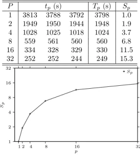
Figure 1: Execution Times and Speedups

are similar).

• Figures 9 and 10 (corresponding to Figures 9 and 10 of [4]) reporting on the impact of retrials on the average profit rate (AP R) and on the average number of busy channels (mC) show for the first parameter set ρ

= 0.4, p

= 0.8 the same results as originally reported; however for the two other parameter sets our experiments report significantly lower figures, i.e., the three lines are much farther apart than in [4].

Since in all other cases the results are identical to the other reports and we have both carefully checked our model and the deviating experiments, the possibility remains that the errors are in solvers of the MOSEL and PRISM. One should know that these details are hidden and we have no information about the solution methods.

As for the time needed for executing the analysis, Figure 1 lists the times (in seconds) for performing all the 920 PRISM runs illustrated in Figures 2–10 with P processes, 1 ≤ P ≤ 32 (the maximum number of processor cores available to us for this experiment). The analysis was performed five times from which we have excluded the fastest and the slowest run. This leads to three values for the execution time t

with average execution time T

; the speedup for this average is reported as S

.

We see that significant speedups up to a maximum of 15.3 can be achieved.

The main reason that from P = 16 to P = 32 the speedup does not grow so

much any more is that we have have attached to every Java thread that executes

n= 8 n= 16 n= 24 n= 32 0

0.2 0.4 0.6 0.8 1

0.5 1 1.5 2 2.5 3 3.5 4 4.5

Pblock

ρ0

n= 8 n= 16 n= 24 n= 32

0 10 20 30 40 50 60

0.5 1 1.5 2 2.5 3 3.5 4 4.5

mQ

ρ0 n= 8

n= 16 n= 24 n= 32

0 50 100 150 200 250

0.5 1 1.5 2 2.5 3 3.5 4 4.5

mTQ

ρ0

n= 8 n= 16 n= 24 n= 32

0 0.1 0.2 0.3 0.4 0.5 0.6 0.7 0.8

0.5 1 1.5 2 2.5 3 3.5 4 4.5

mO

ρ0 n= 8

n= 16 n= 24 n= 32

0 0.2 0.4 0.6 0.8 1 1.2 1.4 1.6 1.8

0.5 1 1.5 2 2.5 3 3.5 4 4.5

mTO

ρ0

n= 8 n= 16 n= 24 n= 32

0 2 4 6 8 10 12 14 16 18

0.5 1 1.5 2 2.5 3 3.5 4 4.5

mAS

ρ0

Figure 2: Performance Measures Without Renting (cf. Fig. 2 from [4])

one instance of PRISM by the command line option -XX:ParallelGCThreads a number of garbage collection threads that concurrently reclaim the memory of objects that are not accessible any more; since the experiment was performed on only 32 processor cores; the number of concurrently executing threads thus significantly exceeded the number of cores. With more cores available, we can expect also for P = 32 a considerably higher speedup.

4. Conclusions

We have shown in this report how the PRISM analysis of a non-trivial mobile

cellular network can be efficiently performed on a modern high performance com-

t1 = 1 t1 = 2 t1 = 3 t1 = 4 0.0001

0.001 0.01 0.1

0.5 1 1.5 2 2.5 3 3.5 4 4.5

Pblock

ρ0

t1 = 1 t1 = 2 t1 = 3 t1 = 4 0.0001

0.001 0.01 0.1

0.5 1 1.5 2 2.5 3 3.5 4 4.5

mQ

ρ0

t1 = 1 t1 = 2 t1 = 3 t1 = 4 0.0001

0.001 0.01 0.1

0.5 1 1.5 2 2.5 3 3.5 4 4.5

mO

ρ0

t1 = 1 t1 = 2 t1 = 3 t1 = 4 0.0001

0.001 0.01 0.1

0.5 1 1.5 2 2.5 3 3.5 4 4.5

mTQ

ρ0

t1 = 1 t1 = 2 t1 = 3 t1 = 4 0.0001

0.001 0.01 0.1

0.5 1 1.5 2 2.5 3 3.5 4 4.5

mTO

ρ0

t1 = 1 t1 = 2 t1 = 3 t1 = 4 5

6 7 8 9 10

0.5 1 1.5 2 2.5 3 3.5 4 4.5

mAS

ρ0

t1 = 1 t1 = 2 t1 = 3 t1 = 4 0.5

1 1.5 2 2.5 3 3.5 4 4.5

0.5 1 1.5 2 2.5 3 3.5 4 4.5

mB

ρ0

t1 = 1 t1 = 2 t1 = 3 t1 = 4 15

20 25 30 35 40 45 50 55

0.5 1 1.5 2 2.5 3 3.5 4 4.5

mC

ρ0

Figure 3: Performance Measures for

(cf. Fig. 3 from [4])

t1 = 1 t1 = 2 t1 = 3 t1 = 4

0 0.1 0.2 0.3 0.4 0.5 0.6 0.7 0.8 0.9 1

0.5 1 1.5 2 2.5 3 3.5 4 4.5

Pb

ρ0

t1 = 1 t1 = 2 t1 = 3 t1 = 4

0 0.1 0.2 0.3 0.4 0.5 0.6 0.7 0.8 0.9 1

0.5 1 1.5 2 2.5 3 3.5 4 4.5

Pb

ρ0 t1 = 1

t1 = 2 t1 = 3 t1 = 4

0 0.1 0.2 0.3 0.4 0.5 0.6 0.7 0.8 0.9 1

0.5 1 1.5 2 2.5 3 3.5 4 4.5

Pb

ρ0

t1 = 1 t1 = 2 t1 = 3 t1 = 4

0 0.1 0.2 0.3 0.4 0.5 0.6 0.7 0.8 0.9 1

0.5 1 1.5 2 2.5 3 3.5 4 4.5

Pb

ρ0

Figure 4: Further Performance Measures for

(cf. Fig. 4 from [4])

puting system and how by this analysis the results performed with the older (and not any more supported) MOSEL-2 tool can be essentially confirmed. However, as already reported in [8], a crucial difference between MOSEL-2 and PRISM (the existence respectively lack of zero-time/infinite-rate transitions) makes the PRISM model somewhat more unhandy than originally thought; more efforts are needed in PRISM to express the desired models in an economical way.

Furthermore, while most of the originally reported results (25 of 29 experiments) could be confirmed, still some discrepancies (in 4 experiments) have to be resolved.

While the error may well be in the PRISM model or its analysis, it might as well be true that there are errors in the originally reported results (we have asked one author of the original paper for a re-examination of these experiments). This demonstrates that the performance analysis of computing systems by analyzing system models alone cannot give full confidence in the correctness of the results:

further verification (by comparison against measurements of the actual system) or

validation (by comparison with the analysis of another model by another tool) is

highly recommended.

t2 = 5 t2 = 6 t2 = 7 t2 = 8

0.01 0.1 1

0 0.5 1 1.5 2 2.5 3 3.5 4

mB

ρ0

t2 = 5 t2 = 6 t2 = 7 t2 = 8

0.0001 0.001 0.01

0 0.5 1 1.5 2 2.5 3 3.5 4

Pblock

ρ0 t2 = 5

t2 = 6 t2 = 7 t2 = 8

0.0001 0.001

0 0.5 1 1.5 2 2.5 3 3.5 4

mQ

ρ0

t2 = 5 t2 = 6 t2 = 7 t2 = 8

0.0001 0.001

0 0.5 1 1.5 2 2.5 3 3.5 4

mO

ρ0 t2 = 5

t2 = 6 t2 = 7 t2 = 8

0.0001 0.001 0.01

0 0.5 1 1.5 2 2.5 3 3.5 4

mTQ

ρ0

t2 = 5 t2 = 6 t2 = 7 t2 = 8

0.0001 0.001 0.01

0 0.5 1 1.5 2 2.5 3 3.5 4

mTO

ρ0

Figure 5: Performance Measures for

(cf. Fig. 5 from [4])

t2 = 5, d= 1 t2 = 5, d= 2 t2 = 5, d= 4 t2 = 5, d= 8 t2 = 8, d= 1 t2 = 8, d= 2 t2 = 8, d= 4 t2 = 8, d= 8 7

7.4 7.8 8.2 8.7

0 0.5 1 1.5 2 2.5 3 3.5 4

APR

t1

Figure 6:

vs.

and

for

(cf. Fig. 6 from [4])

t2 = 5, d= 1 t2 = 5, d= 2 t2 = 5, d= 4 t2 = 5, d= 8 t2 = 8, d= 1 t2 = 8, d= 2 t2 = 8, d= 4 t2 = 8, d= 8 10

15 20 25 30 35 40

0 0.5 1 1.5 2 2.5 3 3.5 4

APR

t1

Figure 7:

vs.

and

for

(cf. Fig. 7 from [4])

t2 = 8, d= 8 t2 = 5, d= 8 t2 = 8, d= 1 t2 = 5, d= 1

5 10 15 20 25 30 35 40

0.5 1 1.5 2 2.5 3 3.5 4 4.5

APR

ρ0

Figure 8:

vs.

and

(cf. Fig. 8 from [4])

po= 0.4, pio= 0.8 po= 0.2, pio= 0.4 po'0, pio'0

25.5 25.55 25.6 25.65 25.7 25.75 25.8 25.85 25.9

4.55 4.56 4.57 4.58 4.59 4.6

APR

ρ0

Figure 9: Impact of retrials on

(cf. Fig. 9 from [4])

po= 0.4, pio= 0.8 po= 0.2, pio= 0.4 po'0, pio'0

41.5 41.55 41.6 41.65 41.7 41.75 41.8 41.85 41.9 41.95 42 42.05 42.1 42.15 42.2 42.25

4.55 4.56 4.57 4.58 4.59 4.6

mC

ρ0

Figure 10: Impact of retrials on the average number of busy chan- nels (cf. Fig. 9 from [4])

Acknowledgment

The publication was supported by the TÁMOP 4.2.2. C-11/1/KONV-2012-0001 project. The project has been supported by the European Union, co-financed by the European Social Fund.

The authors are grateful to the reviewers for their comments and suggestions which improved the quality of the paper.

References

[1] K. Begain, G. Bolch, and Herold H. Practical Performance Modeling Application of the MOSEL Language. Kluwer Academic Publisher, 2012.

[2] T. V. Do, N. H. Do, and R. Chakka. A New Queueing Model for Spectrum Renting in Mobile Cellular Networks. Computer Communications, 35:1165–1171, 2012.

[3] T. V. Do, N.H. Do, and J. Zhang. An Enhanced Algorithm to Solve Multiserver Retrial Queueing Systems with Impatient Customers. Computers & Industrial Engineering, 65(4):719–728, 2013.

[4] T. V. Do, P. Wüchner, T. Bérczes, J. Sztrik, and H. de Meer. A New Finite- Source Queueing Model for Mobile Cellular Networks Applying Spectrum Renting.

Asia-Pacific Journal of Operational Research, 31(2):14400004, 2014. 19 pages, DOI:

10.1142/S0217595914400041.

[5] N. Gharbi, B. Nemmouchi, L. Mokdad, and J. Ben-Othma. The Impact of Breakdowns Disciplines and Repeated Attempts on Performances of Small Cell Networks. Journal of Computational Science, 2014. http://dx.doi.org/10.1016/j.jocs.2014.02.011.

[6] M. Kwiatkowska, G. Norman, and D. Parker. PRISM 4.0: Verification of Probabilistic

Real-time Systems. In G. Gopalakrishnan and S. Qadeer, editors, Proc. 23rd Interna-

[7] PRISM — Probabilistic Symbolic Model Checker, 2013.

prismmodelchecker.org.

[8] W. Schreiner, N. Popov, T. Bérczes, J. Sztrik, and G. Kusper. Applying High Per- formance Computing to Analyzing by Probabilistic Model Checking Mobile Cellular Networks with Spectrum Renting. Technical report, Research Institute for Symbolic Computation (RISC), Johannes Kepler University Linz, Austria, July 2013.

[9] Wolfgang Schreiner. Initial Results on Modeling in PRISM Mobile Cellular Networks with Spectrum Renting. Technical report, Research Institute for Symbolic Computa- tion (RISC), Johannes Kepler University Linz, Austria, March 2013.

A. The PRISM model without spectrum renting

// --- // Spectrum0.prism

// A model for mobile cellular networks.

//

// The model serves as the comparison basis for the improvements // introduced by the application of "spectrum renting" in //

// Tien v. Do, Patrick Wüchner, Tamas Berczes, Janos Sztrik, // Hermann de Meer: A New Finite-Source Queueing Model for // Mobile Cellular Networks Applying Spectrum Renting, // September 2012.

//

// Use for fastest checking the "Sparse" engine and the "Gauss-Seidel"

// solver and switch off "use compact schemes".

//

// Author: Wolfgang Schreiner <Wolfgang.Schreiner@risc.jku.at>

// Copyright (C) 2013, Research Institute for Symbolic Computation // Johannes Kepler University, Linz, Austria, http://www.risc.jku.at // --- // continuous time markov chain (ctmc) model

ctmc

// --- // system parameters

// --- // bounds

const int K = 100; // population size

const int n; // number of servers/channels // rates

const double rho; // normalized traffic intensity const double mu = 1/53.22; // service rate

const double lambda = rho*n*mu/K; // call generation rate const double nu = 1; // retrial rate

const double eta = 1/300; // rate of queueing users // getting impatient

// probabilities

const double p_b = 0.1; // prob. that user gives up // (-> sources)

const double p_q = 0.5; // prob. that user presses button // (-> queue)

const double p_o = 1-p_b-p_q; // prob. that user retries later // (-> orbit)

const double p_io = 0.8; // prob. that impatient user retries // later (-> orbit)

const double p_is = 1-p_io; // prob. that impantient user gives up // (-> sources)

// --- // system model

// note that the order of the modules influences model checking time // heuristically, this seems to be the best one

// --- // available servers accept requests

module Servers

servers: [0..n] init 0;

[sservers] servers < n -> (servers’ = servers+1);

[oservers] servers < n -> (servers’ = servers+1);

[ssources1] servers > 0 & queue = 0 ->

servers*mu : (servers’ = servers-1);

[ssources2] servers > 0 ->

servers*mu : true ; endmodule

// generate requests at rate sources*lambda module Sources

sources: [0..K] init K;

[sservers] sources > 0 ->

sources*lambda : (sources’ = sources-1);

[sorbit] sources > 0 & servers = n ->

sources*lambda*p_o : (sources’ = sources-1);

[squeue] sources > 0 & servers = n ->

sources*lambda*p_q : (sources’ = sources-1);

[ssources1] sources < K -> (sources’ = sources+1);

[ssources2] sources < K -> (sources’ = sources+1);

[qsources] sources < K -> (sources’ = sources+1);

[osources] sources < K -> (sources’ = sources+1);

endmodule

// if no server is available, requests are redirected // with probability p_o to the orbit

formula orbit = K-(sources+servers+queue); // make variable virtual module Orbit

// orbit: [0..K-n] init 0;

[sorbit] orbit < K-n -> true;

[qorbit] orbit < K-n -> true;

[oservers] orbit > 0 -> orbit*nu : true;

[oqueue] orbit > 0 & servers = n -> orbit*nu*p_q : true;

[osources] orbit > 0 & servers = n -> orbit*nu*p_b : true;

endmodule

// with probability p_q to the queue module Queue

queue: [0..K-n] init 0;

[squeue] queue < K-n -> (queue’ = queue+1);

[oqueue] queue < K-n -> (queue’ = queue+1);

[qorbit] queue > 0 & servers = n ->

queue*eta*p_io : (queue’ = queue-1);

[qsources] queue > 0 & servers = n ->

queue*eta*p_is : (queue’ = queue-1);

[ssources2] queue > 0 -> (queue’ = queue-1);

endmodule

// --- // system rewards

// --- // mean number of active requests

rewards "mM"

true : max(0, orbit)+queue+servers;

endrewards

// mean number of calls in orbit rewards "mO"

true : max(0, orbit);

endrewards

// mean number of calls in queue rewards "mQ"

true: queue;

endrewards

// mean number of active calls rewards "mC"

true: servers;

endrewards

// --- // Spectrum0.props

// --- // mean number of active requests

"mM" : R{"mM"}=? [ S ] ; // mean number of active sources

"mK" : K-"mM" ;

// mean throughput (served and unserved)

"m1" : "mK"*lambda ;

// mean number of active calls

"mC" : R{"mC"}=? [ S ] ; // mean goodput

"m1good" : "mC"*mu ;

// probability that arriving customer gets served

"Pgood" : "m1good"/"m1" ;

// mean response time (served and unserved)

"mT" : "mM"/"m1" ;

// mean number of idle servers

"mAS" : n-"mC" ;

// utilization of available servers

"Sutil" : "mC"/n ; // blocking probability

"Pblock" : S=? [ servers = n ] ; // mean queue length

"mQ" : R{"mQ"}=? [ S ] ; // mean time spent in queue

"mTQ" : "mQ" / "m1" ; // mean orbit length

"mO" : R{"mO"}=? [ S ] ; // mean time spent in orbit

"mTO" : "mO" / "m1" ;

B. The PRISM model with spectrum renting

// --- // Spectrum.prism

// A model for mobile cellular networks applying spectrum renting.

//

// The model is described in //

// Tien v. Do, Patrick Wüchner, Tamas Berczes, Janos Sztrik, // Hermann de Meer: A New Finite-Source Queueing Model for // Mobile Cellular Networks Applying Spectrum Renting, // September 2012.

//

// Use for fastest checking the "Sparse" engine and the "Gauss-Seidel"

// solver and switch off "use compact schemes".

//

// Author: Wolfgang Schreiner <Wolfgang.Schreiner@risc.jku.at>

// Copyright (C) 2013, Research Institute for Symbolic Computation // Johannes Kepler University, Linz, Austria, http://www.risc.jku.at // --- // continuous time markov chain (ctmc) model

ctmc

// ---

// renting tresholds

const int t1; // block renting treshold const int t2 = 6; // block release treshold // bounds

const int K = 100; // population size

const int r = 8; // number of servers/channels per block const int m = 5; // maximum number of blocks that can be rented const int n = 2*r; // minimum number of servers/channels

const int M = n+r*m; // maximum number of simultaneous calls // rates

const double rho; // normalized traffic intensity const double mu = 1/53.22; // service rate

const double lambda = rho*n*mu/K; // call generation rate const double nu = 1; // retrial rate

const double eta = 1/300; // rate of queueing users getting // impatient

const double lam_r = 1/5; // block renting rate const double nu_r = 1/7; // block rental retrial rate const double mu_r = 1; // block release reate // probabilities

const double p_b = 0.1; // prob. that user gives up (-> sources) const double p_q = 0.5; // prob. that user presses button

// (-> queue)

const double p_o = 1-p_b-p_q; // prob. that user retries later // (-> orbit)

const double p_io = 0.8; // prob. that impatient user retries // later (-> orbit)

const double p_is = 1-p_io; // prob. that impantient user gives up // (-> sources)

const double p_r = 0.8; // block rental success probability const double p_f = 1-p_r; // block rental failure probability // --- // system model

// note that the order of the modules influences model checking time // heuristically, this seems to be the best one

// --- // number of currently available servers/channels

formula servAvail = n+blocks*r;

// blocks are rented at rate lam_r and released at rate mu_r // renting is successful with probability p_r and fails with

// probability p_f retrying a failed attempt is performed at rate nu_r module Blocks

blocks: [0..m] init 0;

trial: [0..1] init 0;

[success1] trial = 0 & servAvail-servers <= t1 & blocks < m & queue=0 ->

lam_r*p_r: (blocks’ = blocks+1);

[success2] trial = 0 & servAvail-servers <= t1 & blocks < m ->

lam_r*p_r: (blocks’ = blocks+1);

[failure] trial = 0 & servAvail-servers <= t1 & blocks < m ->

lam_r*p_f: (trial’ = 1);

[retrial1] trial = 1 & servAvail-servers <= t1 & blocks < m & queue=0 ->

nu_r*p_r : (trial’ = 0) & (blocks’ = blocks+1) ;

[retrial2] trial = 1 & servAvail-servers <= t1 & blocks < m ->

nu_r*p_r : (trial’ = 0) & (blocks’ = blocks+1) ; [interrupt] trial = 1 & servAvail-servers > t1 ->

9999 : (trial’ = 0); // "immediately"

[release] servAvail-servers >= t2+r & blocks > 0 ->

mu_r : (blocks’ = blocks-1);

endmodule

// available servers accept requests module Servers

servers: [0..M] init 0;

[sservers] servers < servAvail -> (servers’ = servers+1);

[oservers] servers < servAvail -> (servers’ = servers+1);

[success2] servers < M -> (servers’ = servers+1);

[retrial2] servers < M -> (servers’ = servers+1);

[ssources1] servers > 0 & queue = 0 ->

servers*mu : (servers’ = servers-1);

[ssources2] servers > 0 ->

servers*mu : true ; endmodule

// generate requests at rate sources*lambda module Sources

sources: [0..K] init K;

[sservers] sources > 0 ->

sources*lambda : (sources’ = sources-1);

[sorbit] sources > 0 & servers = servAvail ->

sources*lambda*p_o : (sources’ = sources-1);

[squeue] sources > 0 & servers = servAvail ->

sources*lambda*p_q : (sources’ = sources-1);

[ssources1] sources < K -> (sources’ = sources+1);

[ssources2] sources < K -> (sources’ = sources+1);

[qsources] sources < K -> (sources’ = sources+1);

[osources] sources < K -> (sources’ = sources+1);

endmodule

// if no server is available, requests are redirected // with probability p_o to the orbit

formula orbit = K-(sources+servers+queue); // make variable virtual module Orbit

// orbit: [0..K-n] init 0;

[sorbit] orbit < K-n -> true;

[qorbit] orbit < K-n -> true;

[oservers] orbit > 0 -> orbit*nu : true;

[oqueue] orbit > 0 & servers = servAvail -> orbit*nu*p_q : true;

[osources] orbit > 0 & servers = servAvail -> orbit*nu*p_b : true;

endmodule

// if no server is available, requests are redirected // with probability p_q to the queue

module Queue

[oqueue] queue < K-n -> (queue’ = queue+1);

[qorbit] queue > 0 & servers = servAvail ->

queue*eta*p_io : (queue’ = queue-1);

[qsources] queue > 0 & servers = servAvail ->

queue*eta*p_is : (queue’ = queue-1);

[ssources2] queue > 0 -> (queue’ = queue-1);

[success2] queue > 0 -> (queue’ = queue-1);

[retrial2] queue > 0 -> (queue’ = queue-1);

endmodule

// --- // system rewards

// --- // mean number of active requests

rewards "mM"

true : max(0, orbit)+queue+servers;

endrewards

// mean number of calls in orbit rewards "mO"

true : max(0, orbit);

endrewards

// mean number of calls in queue rewards "mQ"

true: queue;

endrewards

// mean number of active calls rewards "mC"

true: servers;

endrewards

// mean number of active blocks rewards "mB"

true: blocks;

endrewards

// --- // Spectrum.props

// --- // mean number of active requests

"mM" : R{"mM"}=? [ S ] ; // mean number of active sources

"mK" : K-"mM" ;

// mean throughput (served and unserved)

"m1" : "mK"*lambda ;

// mean number of active calls

"mC" : R{"mC"}=? [ S ] ;

// mean goodput

"m1good" : "mC"*mu ;

// probability that arriving customer gets served

"Pgood" : "m1good"/"m1" ;

// mean response time (served and unserved)

"mT" : "mM"/"m1" ;

// mean number of rented blocks

"mB" : R{"mB"}=? [ S ] ;

// mean number of available servers

"mS" : n+"mB"*r ;

// mean number of idle servers

"mAS" : "mS"-"mC" ;

// utilization of available servers

"Sutil" : "mC"/"mS" ; // blocking probability

"Pblock" : S=? [ servers = servAvail ] ; const int B;

// probability that B blocks are partially utilized

"Pb" : S=? [ n+r*(B-1) < servers & servers <= n+r*B ] ; // mean queue length

"mQ" : R{"mQ"}=? [ S ] ; // mean time spent in queue

"mTQ" : "mQ" / "m1" ; // mean orbit length

"mO" : R{"mO"}=? [ S ] ; // mean time spent in orbit

"mTO" : "mO" / "m1" ; const int d;

// average profit rate

"APR" : "mC" - (r/d) * "mB" ;

C. The parallel execution script

#!/bin/sh

# the program locations export PRISM_JAVA="prism-java"

PRISM="prism"

# the input/output locations MODELFILE="Spectrum.prism"

MODELFILE0="Spectrum0.prism"

MODELFILE2="Spectrum2.prism"

MODELFILE3="Spectrum3.prism"

PROPSFILE="Spectrum.props"

PROPSFILE0="Spectrum0.props"

RESULTDIR="Results"

LOGDIR="Logfiles"

LOGFILE="LOGFILE"

# the checker settings

PRISMOPTIONS="-sparse -gaussseidel -nocompact"

# the number of processes to be used for PROC in 1 2 4 8 16 32 ; do (

# the properties to be checked and the parameters for the experiment

# Figure 2

for PROPERTY in Pblock mO mTO mQ mTQ mAS ; do for RHO in $(seq 0.6 0.5 4.6) ; do

for N in 8 16 24 32 ; do

echo "$PRISM $PRISMOPTIONS $MODELFILE0 $PROPSFILE0 -prop $PROPERTY \ -const rho=$RHO,n=$N \

-exportresults $RESULTDIR/Fig2-$PROPERTY-$N-$RHO \

> $LOGDIR/Fig2-$PROPERTY-$N-$RHO"

done done done

# Figure 3

for PROPERTY in Pblock mO mTO mB mQ mTQ mC mAS ; do for RHO in $(seq 0.6 0.5 4.6) ; do

for T1 in $(seq 1 1 4) ; do

echo "$PRISM $PRISMOPTIONS $MODELFILE $PROPSFILE -prop $PROPERTY \ -const rho=$RHO,t1=$T1 \

-exportresults $RESULTDIR/Fig3-$PROPERTY-$T1-$RHO \

> $LOGDIR/Fig3-$PROPERTY-$T1-$RHO"

done done done

# Figure 4 PROPERTY="Pb"

for B in $(seq 1 1 4) ; do

for RHO in $(seq 0.6 0.5 4.6) ; do for T1 in $(seq 1 1 4) ; do

echo "$PRISM $PRISMOPTIONS $MODELFILE $PROPSFILE -prop $PROPERTY \ -const B=$B,rho=$RHO,t1=$T1 \

-exportresults $RESULTDIR/Fig4-$PROPERTY-$B-$T1-$RHO \

> $LOGDIR/Fig4-$PROPERTY-$B-$T1-$RHO"

done done done

# Figure 5 RHO="0.6"

for PROPERTY in mB Pblock mQ mO mTQ mTO ; do for T1 in $(seq 0 1 4) ; do

for T2 in $(seq 5 1 8) ; do

echo "$PRISM $PRISMOPTIONS $MODELFILE2 $PROPSFILE -prop $PROPERTY \ -const rho=$RHO,t1=$T1,t2=$T2 \

-exportresults $RESULTDIR/Fig5-$PROPERTY-$T1-$T2 \

> $LOGDIR/Fig5-$PROPERTY-$T1-$T2"

done done done

# Figures 6-7 PROPERTY="APR"

for RHO in 0.6 4.6 ; do for T1 in $(seq 0 1 4) ; do

for T2 in 5 8 ; do for D in 1 2 4 8 ; do

echo "$PRISM $PRISMOPTIONS $MODELFILE2 $PROPSFILE -prop $PROPERTY \ -const rho=$RHO,t1=$T1,t2=$T2,d=$D \

-exportresults $RESULTDIR/Fig67-$PROPERTY-$T1-$T2-$D-$RHO \

> $LOGDIR/Fig67-$PROPERTY-$T1-$T2-$D-$RHO"

done done done done

# Figure 8, T1 apparently 2 PROPERTY="APR"

T1=2

for RHO in $(seq 0.6 0.5 4.6) ; do for T2 in 5 8 ; do

for D in 1 8 ; do

echo "$PRISM $PRISMOPTIONS $MODELFILE2 $PROPSFILE -prop $PROPERTY \ -const rho=$RHO,t1=$T1,t2=$T2,d=$D \

-exportresults $RESULTDIR/Fig8-$PROPERTY-$T2-$D-$RHO \

> $LOGDIR/Fig8-$PROPERTY-$T2-$D-$RHO"

done done done

# Figures 9,10 PROPERTY="APR"

T1=2 T2=5 D=2

for PROPERTY in "APR" "mC" ; do PO=0.2

PIO=0.4

for RHO in $(seq 4.55 0.01 4.6) ; do

-exportresults $RESULTDIR/Fig910-$PROPERTY-$PO-$PIO-$RHO \

> $LOGDIR/Fig910-$PROPERTY-$PO-$PIO-$RHO"

done PO=0.4 PIO=0.8

for RHO in $(seq 4.55 0.01 4.6) ; do

echo "$PRISM $PRISMOPTIONS $MODELFILE3 $PROPSFILE -prop $PROPERTY \ -const rho=$RHO,t1=$T1,t2=$T2,d=$D,p_o=$PO,p_io=$PIO \

-exportresults $RESULTDIR/Fig910-$PROPERTY-$PO-$PIO-$RHO \

> $LOGDIR/Fig910-$PROPERTY-$PO-$PIO-$RHO"

done

PO=0.000000001 PIO=0.000000001

for RHO in $(seq 4.55 0.01 4.6) ; do

echo "$PRISM $PRISMOPTIONS $MODELFILE3 $PROPSFILE -prop $PROPERTY \ -const rho=$RHO,t1=$T1,t2=$T2,d=$D,p_o=$PO,p_io=$PIO \

-exportresults $RESULTDIR/Fig910-$PROPERTY-$PO-$PIO-$RHO \

> $LOGDIR/Fig910-$PROPERTY-$PO-$PIO-$RHO"

done done

# execute the experiments in parallel with PROC processes ) | $TIME -p $PARALLEL $PROC > $LOGDIR/$LOGFILE 2>&1 done