Probabilistic joint inversion of waveforms and polarity data for double-couple focal mechanisms of local earthquakes

(1)

Advance Access publication 2018 March 13 GJI Seismology

Probabilistic joint inversion of waveforms and polarity data for double-couple focal mechanisms of local earthquakes

Zolt´an W´eber

K¨ovesligethy Rad´o Seismological Observatory, MTA CSFK GGI, H-1112Budapest, Meredek u.18., Hungary. E-mail:weber@seismology.hu

Accepted 2018 March 12. Received 2018 March 4; in original form 2017 July 19

S U M M A R Y

Estimating the mechanisms of small (M<4) earthquakes is quite challenging. A common scenario is that neither the available polarity data alone nor the well predictable near-station seismograms alone are sufficient to obtain reliable focal mechanism solutions for weak events.

To handle this situation we introduce here a new method that jointly inverts waveforms and polarity data following a probabilistic approach. The procedure called joint waveform and polarity (JOWAPO) inversion maps the posterior probability density of the model parameters and estimates the maximum likelihood double-couple mechanism, the optimal source depth and the scalar seismic moment of the investigated event. The uncertainties of the solution are described by confidence regions. We have validated the method on two earthquakes for which well-determined focal mechanisms are available. The validation tests show that including waveforms in the inversion considerably reduces the uncertainties of the usually poorly constrained polarity solutions. The JOWAPO method performs best when it applies waveforms from at least two seismic stations. If the number of the polarity data is large enough, even single-station JOWAPO inversion can produce usable solutions. When only a few polarities are available, however, single-station inversion may result in biased mechanisms. In this case some caution must be taken when interpreting the results. We have successfully applied the JOWAPO method to an earthquake in North Hungary, whose mechanism could not be estimated by long-period waveform inversion. Using 17 P-wave polarities and waveforms at two nearby stations, the JOWAPO method produced a well-constrained focal mechanism. The solution is very similar to those obtained previously for four other events that occurred in the same earthquake sequence. The analysed event has a strike-slip mechanism with aPaxis oriented approximately along an NE–SW direction.

Key words: Inverse theory; Joint inversion; Probability distributions; Waveform inversion;

Earthquake source observations.

1 I N T R O D U C T I O N

In areas of low-to-moderate seismicity, small-magnitude local earthquakes provide invaluable information on fault parameters and small-scale tectonic structure. The focal mechanisms of small (M< 4) events can be used to infer the structure and kinemat- ics of faults at depth and to constrain the crustal stress field in which the earthquakes occur. Reliably estimating the mechanisms for small events is, however, quite challenging.

Double-couple (DC) focal mechanisms of small events are most often found using first-motion polarities of body waves recorded at local seismic stations (e.g. Reasenberg & Oppenheimer1985;

Hardebeck & Shearer2002; Snoke2003). Since only the binary up or down of the first motions counts in these methods, a dense sampling of the focal sphere is required to form a reliable solution.

For many small earthquakes, however, first-motion observations are

not sufficient, leading to large uncertainties in the retrieved focal mechanisms.

Another possible approach to obtain earthquake focal mechanisms is waveform inversion. Since seismic waveforms contain much more information about the source than the first-motion polarities alone, even sparse data sets may suffice for the task. Because for small events the signal-to-noise ratio (SNR) of the recorded seismograms is poor at long periods, low-magnitude local events have to be analysed at relatively high frequencies (>0.5 Hz). Several procedures have been proposed to estimate the focal mechanism of low-magnitude earthquakes using high-frequency seismograms recorded at local stations (e.g. ˇS´ılen´yet al.1992; Maoet al.1994;

Panza & Sarao2000; Saraoet al.2001; W´eber2005,2006,2009;

Vavryc˘uk & K¨uhn2012). At high frequencies, however, the knowl- edge of the medium is usually not detailed enough to model complex waveforms at large epicentral distances, that is, waveforms can be

(2)

16˚E 16˚E

17˚E 17˚E

18˚E 18˚E

19˚E 19˚E

20˚E 20˚E

21˚E 21˚E

22˚E 22˚E

23˚E 23˚E

46˚N 46˚N

47˚N 47˚N

48˚N 48˚N

49˚N 49˚N

0 km 100 km

AMBH BEHE

BSZH BUD

MORH MPLH

PSZ SOP

TIH CSKK

PKS3

PKS5

PKS6 PKS7

PKS8 PKSG

PKST SUKH

CRVS

CONA

DRGR

GROS

JAVC

SIRR

SMOL VYHS

Szabadszállás Oroszlány

Iliny

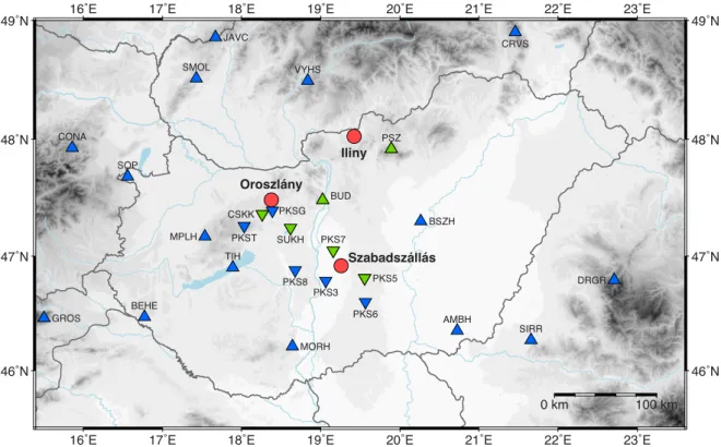
Figure 1.Map of Hungary showing the location of the seismic stations used in this study (triangles: broad-band stations; inverse triangles: short-period stations) and the epicentres of the three earthquakes selected for the application of the proposed joint waveform and polarity (JOWAPO) inversion (red circles).

Green symbols: stations whose waveform recordings are used in the presented calculations. Blue symbols: stations where only polarity data are utilized. Station codes and event locations are also indicated.

Reference Polarities only Pol. + CSKK Pol. + SUKH Pol. + CSKK + SUKH

Oroszlány

2011−01−29 17:41 M_L=4.5

CSKK SUKH CSKK + SUKH

Figure 2.Source mechanism solutions for the Oroszl´any test event (ML=4.5). The mechanism obtained by a 10-station long-period waveform inversion (W´eber2016a) is shown as the reference solution. Additional mechanisms are derived by the proposed JOWAPO method using different data sets as indicated above the beach balls. Compressional quadrants of the optimal solutions are shaded. Contours represent the 50, 68, 90 and 95 per cent confidence zones for the P(red) andT(blue) principal axes. Red triangles and blue inverse triangles denote respectively thePand T axes of the optimal solutions. First-arrivalP-wave polarities are indicated as well (solid circle: compression; open circle: dilatation). Equal area projection of lower hemisphere is used.

modelled satisfactorily only for relatively near stations. Unfortu- nately, the recording seismic network is often not dense enough to provide us with the sufficient number of high-quality near-station waveforms that would be necessary for successful waveform inversion.

Thus, a common scenario is that neither polarity data inversion alone nor the inversion of near-station waveforms alone can produce reliable focal mechanism solutions for small events. Then the idea comes up naturally that waveforms and polarity data should be inverted jointly.

Using both waveforms and polarity data in moment tensor inversion is not a new concept. Guilhemet al.(2014), for example, calculate the full moment tensors of small earthquakes in the Geysers geothermal field using waveform modelling as well as first-motion inversion and then compare the solutions obtained by the two different methods. Alvizuri & Tape (2016) apply a grid-search algorithm to obtain the full moment tensor whose synthetic seismograms provide the best fit to observed seismograms. The grid search is limited to moment tensors whose predicted first-motion polarities all match

(3)

−180

−135

−90

−45 0 45 90 135 180

Polarities only

Rake

0.0 0.5 1.0 1−cos(dip) 0.0

0.5 1.0

0 45 90 135 180 225 270 315 360 Strike

1−cos(dip)

−180

−135

−90

−45 0 45 90 135 180

Polarities + CSFK + SUKH

Rake

0.0 0.5 1.0 1−cos(dip) 0.0

0.5 1.0

0 45 90 135 180 225 270 315 360 Strike

1−cos(dip)

0.0 0.2 0.4 0.6 0.8 1.0

Posterior probability density

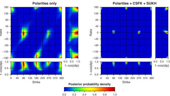
Figure 3. Posterior probability density (PPD) of the source parameters for the Oroszl´any test event (ML=4.5). Left: PPD obtained by the proposed JOWAPO method using polarity data alone. Right: PPD derived using polarities and waveforms observed at two nearby stations, CSKK and SUKH. The presented 2-D marginal probability densities are normalized individually.

the observations. Chianget al.(2014) investigate nuclear explosions using regional moment tensor inversion coupled with network sensitivity solution (NSS) analysis (Fordet al.2010).P-wave polarities are also included in the NSS analysis to better constrain the moment tensor solution. The same procedure is applied in Boyd et al.(2015) and Nayak & Dreger (2015). Fojt´ıkov´a & Zahradn´ık (2014) apply a two-step procedure to obtain the DC mechanisms of small earthquakes. First they calculate a broad range of possible mechanisms using polarity inversion. Then, in the second step, they scan these polarity solutions one by one and select those ones that satisfactorily model a few number of near-station seismograms. A common feature of the above mentioned inversion procedures is that the uncertainties of the resulting focal mechanisms are estimated by accepting all models within a given threshold on the misfit value.

The value of such a threshold is, however, not based on the analysis of the underlying origin of the uncertainty.

In this study we introduce a probabilistic waveform and polarity inversion procedure that estimates the posterior probability density (PPD) of the DC focal mechanisms of local earthquakes by using the information on the model space carried jointly by waveforms and polarity data. The final estimates of the source parameters are given by the maximum likelihood point of the PPD, whereas solution uncertainties are presented by confidence zones. The method can utilize any type of first-motion data (P,SVandSHpolarities) and can invert polarities without waveforms or vice versa.

We first describe the proposed joint waveform and polarity (JOWAPO) inversion technique in detail. Then the method is validated on two earthquakes (M_L =4.5 and M_L = 3) in Hungary, for which the focal mechanisms were previously obtained by waveform inversion. Finally, the method is applied to anML3.9 event in Hungary. Because of the low SNR at low frequencies, long-period waveform inversion of this event was unsuccessful.

2 I N V E R S I O N M E T H O D

For a small earthquake with a sparse data set, our aim cannot be more than to find its most probable DC focal mechanism with its

uncertainty. For this purpose, the most suitable inversion technique is Bayesian sampling. Bayesian sampling generates an ensemble of models (DC focal mechanisms in this case) whose members are dis- tributed according to the PPD of the model parameters. Integrating over certain parameters of this joint PPD yields marginal distributions over arbitrary individual parameters or parameter combinations. The probabilistic JOWAPO method proposed in this paper relies on similar principles.

Following Tarantola (1987), the PPD of the model parameters mgiven the observed datad,σ(m|d), is the product of two terms.

The prior probability densityρ(m) incorporates information about the model parameters that is independent of the observed data.

The second term, the likelihood functionL(d|m), measures the fit between the observed and predicted data.

In our inversion problem, the model parameter vectormincludes the three angular parameters of a DC focal mechanism: the strike φ, dip δ and rake λ. The observed data vector consists of the polarity datapand the waveform dataw. Since polarities and filtered seismograms can be considered independent, the PPD of the model parameters is given by

σ(m|p,w)∝ρ(m)L_p(p|m)Lw(w|m), (1)

where Lp(p|m) and Lw(w|m) are the likelihood functions for polarities and waveforms, respectively.

In the following subsections we give the detailed descriptions of the three terms in eq. (1).

2.1 Prior probability density

We assume no prior information on the model parameters, soρ(m) must represent the null information probability density.

Any fault plane defined by strike and dip can be represented by a unit normal vector. No prior information on this normal vector means that it has equal probability in all directions on the focal sphere. Since a surface element on the unit focal sphere is sinδ· dφ·dδ, the null information probability density of the normal vector is proportional to sinδ. The slip direction is independent of

(4)

d=15.8 a=203931

CSKK_Z

d=15.8 a=377369

CSKK_E

d=15.8 a=591260

CSKK_N

d=32.3 a=50387

SUKH_Z

d=32.3 a=51712

SUKH_E

0 s 10 s

d=32.3 a=86135

SUKH_N

Figure 4.Observed waveforms for the Oroszl´any test event (ML=4.5).

The seismograms are band-pass filtered with cut-off frequencies of 0.5 and 2 Hz. TheP-waves (red) andS-waves (blue) used in the inverse calculations are also depicted. On the left-hand side of each seismogram, station code and component are indicated. The numbers above the waveforms represent epicentral distance in km (d) and peak amplitude in nm (a). Waveforms are normalized individually.

the fault orientation with constant null information probability, so the prior probability density of the model parameters is

ρ(m)∝sinδ. (2)

If instead ofmwe use them^∗=(φ,cosδ, λ) parametrization of the model space, the null information probability density and, consequently, our prior probability density becomes

ρ^∗(m^∗)=ρ(m) ∂m

∂m^∗

=const, (3)

where|∂m/∂m^∗|represents the absolute value of the Jacobian of them→m^∗transformation (Tarantola1987,eq. 1.18).

Since subsequent calculations are more convenient for a parametrization with constant null information probability density, hereafter we use the (φ, cosδ,λ) model parameter vector but, for simplicity, we retain the notation ofmandρ(m):

m=(φ,cosδ, λ) (4)

ρ(m)=const. (5)

2.2 Polarity likelihood

Here we adopt the approach of Brillingeret al. (1980). Let the polarity observation at stationibe defined asp_i =+1 for positive first motion andpi= −1 for negative first motion. Then the polarity

c=15.8 c=0.66 vr=0.42 a=132341

CSKK_Z_P

d=15.8 c=0.88 vr=0.77 a=203931

CSKK_Z_S

d=15.8 c=0.86 vr=0.71 a=57279

CSKK_E_P

d=15.8 c=0.93 vr=0.71 a=175918

CSKK_N_P

d=32.3 c=0.96 vr=0.84 a=46251

SUKH_Z_P

d=32.3 c=0.91 vr=0.82 a=38353

SUKH_E_P

0 s 2 s

d=32.3 c=0.93 vr=0.75 a=40176

SUKH_N_P

0 s 2 s

d=32.3 c=0.72 vr=0.44 a=68294

SUKH_N_S

Figure 5.Waveform comparison for the Oroszl´any test event (ML=4.5).

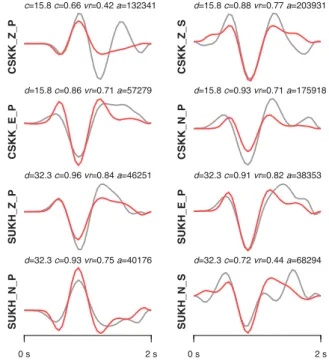
The observed seismograms (grey lines) are band-pass filtered with cut- off frequencies of 0.5 and 2 Hz. The synthetic waveforms (red lines) are computed using the maximum likelihood source parameters obtained by the proposed JOWAPO inversion. On the left-hand side of each seismogram, station code, component and phase are indicated. The numbers above the waveforms represent epicentral distance in km (d), normalized correlation (c), variance reduction (vr) and peak amplitude in nm (a). Waveforms are normalized individually.

likelihood function is

Lp(p|m)=

Np

i=1

πi⁽¹⁺^pⁱ⁾^/²(1−πi)^(1−pⁱ^)/2, (6)

whereN_pdenotes the number of the observed polarity data andπi

is given by

πi =γi+(1−2γi) Ai(m)

σi

. (7)

Here,(·) is the cumulative distribution function of the normal distribution and Ai(m) is the theoretical amplitude of theith first motion observation for a given seismic phase (P,SVorSH) and focal mechanism m. This model has the property that the larger the magnitude ofAi, the greater the probability that the sign of the first motion has been observed correctly (Brillinger et al.1980).

The same model is applied by Walshet al.(2009) and Pughet al.

(2016).

In eq. (7),γi andσi characterize the uncertainty of the polarity data and control the shape of the likelihood function. Theγ parameter (0≤γ ≤0.5) defines the probability that the polarity reading is incorrect, whereas theσparameter (σ >0) describes the modelling errors in calculating the first-motion amplitudes (mostly due to inaccurate crustal models). For precise data, bothγ andσ are small.

(5)

d=16.6 a=628

PKS7_Z

d=16.6 a=2845

PKS7_E

d=16.6 a=2892

PKS7_N

d=25.3 a=336

PKS5_Z

d=25.3 a=1917

PKS5_E

0 s 10 s

d=25.3 a=3124

PKS5_N

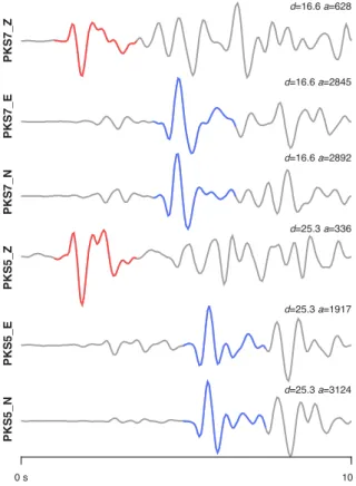
Figure 6.Observed waveforms for the Szabadsz´all´as test event (ML=3.0).

The seismograms are band-pass filtered with cut-off frequencies of 0.5 and 2 Hz. TheP-waves (red) andS-waves (blue) used in the inverse calculations are also depicted. For more details see the caption of Fig.4.

2.3 Waveform likelihood

Here we adopt the Gaussian model, so the waveform likelihood function is given by

Lw(w|m)∝exp

−1

2(g(m,a)−w)^TC⁻¹_W(g(m,a)−w)

, (8)

whereCWdenotes the waveform covariance matrix (representing modelling and observational errors) andg(m,a) is the forward modelling operator that generates the displacement field for a given focal mechanismm. Vectoraincorporates all the important parameters that affect the output of the forward operator, such as the earth model, epicentre coordinates, focal depth, station coordinates and scalar seismic moment.

The covariance matrixCWplays an important role in the inversion and several methods have been proposed for its estimation.

In the simplest case, noise correlation is not taken into account and a diagonal covariance matrix is used (e.g. Yagi & Fukahata 2011; Minsonet al.2013; Kuboet al.2016). Recognizing the cor- related nature of both the observational and modelling errors, some authors consider the full covariance matrix in moment tensor inversion (Duputelet al.2012). For example, the full matrix can be estimated empirically from data residuals (Dettmeret al.2014) or from synthetically generated noise seismograms (Gouveia & Scales 1998; Sambridge1999; Mustać & Tkalc˘ić2016). Moreover, Mustać

& Tkalc˘i´c (2016) and Vack´aˇret al.(2017) use covariance matrix due to observational noise estimated from pre-event data, whereas Hallo & Gallovic˘ (2016) apply approximate formulae to estimate the covariance matrix due to modelling errors (errors in the Green’s functions).

2.4 Mapping the posterior

When solving for a DC focal mechanism using polarity data only, the PPD can be mapped on a sufficiently fine uniform grid defined in the model space (see, e.g. Walshet al.2009). Involving waveforms in the inversion problem, however, makes this approach inefficient.

In this study, the PPD σ(m) in eq. (1) is mapped by the oct- tree importance sampling algorithm (Lomax & Curtis2001). The oct-tree algorithm gives accurate, efficient and complete mapping of the PPD. Initially, it maps the PPD on a coarse regular grid.

Then it uses recursive octal subdivision and sampling of cells in the 3-D model space to generate a cascaded oct-tree structure of sampled cells. The spatial density of sampled cells in the final oct- tree structure follows the PPD: the larger the PPD, the smaller the spatial size and the larger the spatial density of the sampled cells.

After the oct-tree structure has been created with a sufficiently large number of sampled cells, an ensemble of focal mechanism solutions is obtained by drawing random samples from each cell with the number of samples proportional to the probability in that cell.

For each mechanism encountered throughout the above calculations, the scalar moment has to be determined as well. For any point m(DC mechanism) in the 3-D model space, whether it belongs to the oct-tree structure or to the ensemble, we calculate the synthetic waveformss(m,a) assuming unit scalar moment. Then we invert the observed waveformswfor the optimal scalar momentM0in such a way thatM0minimizes theL2norm of the residualw−M0s(m,a).

It can be shown easily that the optimum scalar moment is given by M0=

iwisi(m,a)

isi(m,a)² , (9)

wherewi andsi(m,a) are samples of the data vector ands(m,a), respectively. Then, the forward modelling operatorg(m,a) in eq.

(8) becomes g(m,a)=

iwisi(m,a)

isi(m,a)² s(m,a). (10)

Therefore, the operatorg(m,a) provides both the optimal scalar moment and the synthetic displacement field for a given focal mechanismm.

Up to this point we assumed that the hypocentre of the investigated earthquake was known. Hypocentral depth is, however, usually poorly constrained, so because waveforms are rather sensitive to focal depth, in addition to the parameters describing the focal mechanism, the source depth should also be treated as an unknown parameter. Here we estimate source depth by a grid search made in a vertical line below the epicentre. The generated ensemble of focal mechanism solutions provides uncertainty and covariance information at the best fitting depth.

3 P R A C T I C A L I S S U E S

Waveform data used in the present study were recorded by the Hungarian National Seismological Network (HNSN) and the Paks Microseismic Monitoring Network (PMMN) (Fig.1). Polarity data from the neighbouring countries are also utilized.

As the first step of waveform preparation, all the velocity seismograms are deconvolved from their instrument response and then integrated to displacement. The records are further processed by frequency filtering. To reduce propagation effects as much as possible and get stable and robust results from the inversion, it is crucial to keep the longest possible periods with a good SNR. The lower

(6)

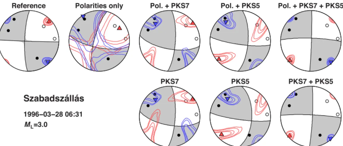
Reference Polarities only Pol. + PKS7 Pol. + PKS5 Pol. + PKS7 + PKS5

Szabadszállás

1996−03−28 06:31

=3.0

PKS7 PKS5 PKS7 + PKS5

M_L

Figure 7.Source mechanism solutions for the Szabadszállás test event (ML=3.0). The mechanism obtained by a six-station short-period waveform inversion (Wéber2016a) is shown as the reference solution. Additional mechanisms are derived by the proposed JOWAPO method using different data sets as indicated above the beach balls. For more details see the caption of Fig.2.

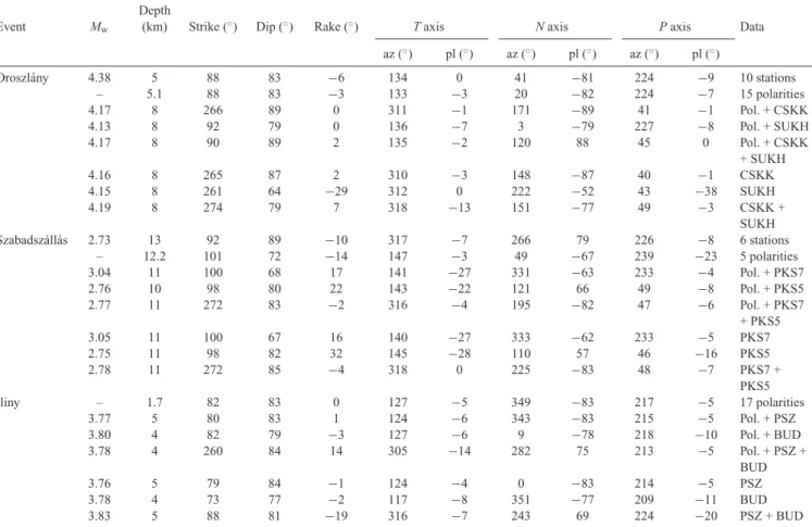
Table 1. Hypocentral parameters of the studied earthquakes.

Event Date Time Lon. Lat. Depth σlon σlat σdepth ML Source

(yyyy-mm-dd) (hh:mm:ss) (^◦E) (^◦N) (km) (km) (km) (km)

Oroszl´any 2011-01-29 17:41:38 18.375 47.482 5.1 0.483 0.831 0.963 4.5 W´eber (2016a)

Szabadszállás 1996-03-28 06:31:22 19.259 46.914 12.2 0.792 0.902 1.354 3.0 Wéber (2016a)

Iliny 2015-01-01 10:45:57 19.422 48.026 1.7 0.765 0.969 0.689 3.9 W´eber (2016b)

σlon,σlat,σdepth: standard deviation of longitude, latitude, and depth, respectively;ML: local magnitude.

cut-off frequency is chosen to avoid the weak long-period signals from small events and the poor long-period response of the short- period instruments, whereas the higher cut-off frequency is selected below the corner frequency of the analysed earthquake. The same filter is applied to both the data and synthetics.

A well-calibrated velocity model is important to obtain robust estimates of the source parameters. In this study we use the 1-D velocity model by Gr´aczer & W´eber (2012) computed from arrival time data of earthquakes and controlled explosions for the territory of Hungary. For constructing the synthetic waveforms (Green’s functions), we employ a frequency–wavenumber integration method (Wang & Herrmann 1980; Herrmann & Wang 1985; Herrmann 2013), which allows calculating the entire wavefield for horizon- tally layered earth structures.

Hallo & Gallovic˘ (2016) illustrate that differences between the true velocity structure and a simple 1-D model mainly affect the arrival times of seismic phases but do not significantly alter the as- sociated waveforms. So we break up the seismograms into segments containing the beginning of theP- andS-wave trains and use these segments in the inversion. A similar approach is followed by, for example, Zhao & Helmberger (1994). For data, the processed time window starts at the observed arrival of the selected phase, whereas for Green’s functions it starts at the theoretical arrival time. The length of the time window is chosen according to the epicentral distance but it is shortened when it becomes evident that the latter part of the seismogram has not been recovered satisfactorily. To avoid waveform complexities that cannot be explained by our 1-D velocity model, we simply discard them and concentrate on data with high-quality waveform fit.

To evaluate the polarity likelihood, we must define the values for the uncertainty parametersγiandσi in eq. (7). For simplicity, we apply the same values for each polarity data used in this study. In a detailed analysis of earthquakes in Southern California, Hardebeck

& Shearer (2002) observed that around 20 per cent of polarity readings were inconsistent. Thus we adopt the rather conservative value ofγ =0.2 (Walshet al.2009). For the amplitude noise, we take a value ofσ= ¹₆ (Brillingeret al.1980; De Nataleet al.1991;

Zollo & Bernard1991).

In this research we do not intend to address the difficult problem of error estimation, so for the data covariance matrixCW in eq. (8) we use a simple diagonal matrix to illustrate our inversion method. Assuming uncorrelated noise, however, can underestimate parameter uncertainties. To reduce this undesirable effect we use conservative estimates on data and modelling errors and adopt the conclusion of Zahradn´ık & Cust´odio (2012) that realistic data errors have the same order of magnitude of the data itself, mostly due to inaccurate crustal models. More specifically, in this study the diagonal elements ofCWcorresponding to the data of a given waveform are chosen to be the mean squared value of that waveform.

After mapping the PPD of the model parameters and obtaining an ensemble of focal mechanism solutions according to the procedure described in Section 2.4, we calculate the principal axes for each member mechanism of the ensemble. Here we adopt the convention of Sipkin (1993) that thePandTaxes always point upwards and the principal axes form a right-handed coordinate system. Then we construct the 2-D histograms of the principal axes on the focal sphere and determine the confidence zones for the 50, 68, 90 and 95 per cent confidence levels. Finally, to illustrate the uncertainties of the focal mechanism solution, we plot the confidence contours of thePandTprincipal axes on top of the beach ball representation of the maximum likelihood mechanism.

In addition to the principal axes, we also deduce the faulting style for the members of the ensemble applying the classification scheme of Zoback (1992). Three main faulting styles are defined: normal faulting (NF) when thePaxis is vertical andTis horizontal; strike- slip (SS) when bothPandTare horizontal; and thrust faulting (TF)

(7)

−180

−135

−90

−45 0 45 90 135 180

Polarities only

Rake

0.0 0.5 1.0 1−cos(dip) 0.0

0.5 1.0

0 45 90 135 180 225 270 315 360 Strike

1−cos(dip)

−180

−135

−90

−45 0 45 90 135 180

Polarities + PKS7 + PKS5

Rake

0.0 0.5 1.0 1−cos(dip) 0.0

0.5 1.0

0 45 90 135 180 225 270 315 360 Strike

1−cos(dip)

0.0 0.2 0.4 0.6 0.8 1.0

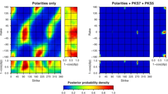
Figure 8.Posterior probability density (PPD) of the source parameters for the Szabadsz´all´as test event (ML=3.0). Left: PPD obtained by the proposed JOWAPO method using polarity data alone. Right: PPD derived using polarities and waveforms observed at two nearby stations, PKS7 and PKS5. The presented 2-D marginal probability densities are normalized individually.

d=16.6 c=0.97 vr=0.94 a=583

PKS7_Z_P

d=16.6 c=0.98 vr=0.97 a=2845

PKS7_E_S

d=16.6 c=0.84 vr=0.71 a=2892

PKS7_N_S

d=25.3 c=0.93 vr=0.85 a=336

PKS5_Z_P

0.0 s 2.5 s

d=25.3 c=0.81 vr=0.65 a=1917

PKS5_E_S

0.0 s 2.5 s

d=25.3 c=0.87 vr=0.76 a=3124

PKS5_N_S

Figure 9. Waveform comparison for the Szabadsz´all´as test event (ML=3.0). The observed seismograms (grey lines) are band-pass filtered with cut-off frequencies of 0.5 and 2 Hz. For more details see the caption of Fig.5.

whenPis horizontal andTis vertical. The World Stress Map Project also uses the intermediate cases transtension (NS) and transpression (TS) for the combination of SS faulting with NF and TF, respectively.

Thus the ensemble of focal mechanisms produced by the proposed JOWAPO inversion can be characterized by the percentages of the different faulting styles appearing in the ensemble.

4 T E S T I N G T H E M E T H O D

In this section we test the proposed JOWAPO method on two earthquakes in Hungary whose focal mechanisms have already been obtained by waveform inversion. TheML4.5 Oroszlány event occurred in the most seismically active region in Hungary and was well recorded on seismic stations in the HNSN and across eastern and central Europe (Wéber & Süle2014). TheML3 Szabadszállás

d=37.2 a=1804

PSZ_Z

d=37.2 a=7566

PSZ_E

d=37.2 a=9123

PSZ_N

d=67.2 a=413

BUD_Z

d=67.2 a=601

BUD_E

0 s 14 s

d=67.2 a=759

BUD_N

Figure 10.Observed waveforms for the Iliny event (ML=3.9). The seismograms are band-pass filtered with cut-off frequencies of 0.4 and 0.8 Hz.

TheP-waves (red) used in the inverse calculations are also depicted. For more details see the caption of Fig.4.

event in central Hungary, on the other hand, was recorded only by a local network. The test events and the seismic stations used in the subsequent inverse calculations are shown in Fig.1. The hypocentral parameters of the earthquakes are listed in Table1.

(8)

4.1 The Oroszl ´any test event

Applying a probabilistic waveform inversion algorithm, Wéber (2016a) estimated the source mechanism of the Oroszlány test event using local and near-regional long-period (8–20 s) waveform data of 10 stations in Hungary and neighbouring countries. His solution shows very good agreement with the regional moment tensors published in the online catalogues of the U.S. Geological Sur- vey National Earthquake Information Center, the German Research Centre for Geosciences, and the Istituto Nazionale di Geofisica e Vulcanologia. The 10-station mechanism of Wéber (2016a), taken as the reference solution for the present research, is described in Table2and shown in Fig.2. The earthquake is an SS event, typical for the compressional regime of the Pannonian basin (Badaet al.

1999,2007).

As a first step, we estimated the source mechanism using only the 15 availableP-wave polarities and accepting the focal depth derived from arrival times (Table1). The optimal JOWAPO solution is very close to the reference mechanism (Table2) but it has considerable uncertainty. The uncertainties of theP and T principal axes are illustrated in Fig.2by the contours of the 50, 68, 90 and 95 per cent confidence regions. These confidence regions show that the solution is most probably an SS event, but it may be even NF with considerable probability. Indeed, applying the classification scheme of Zoback (1992) reveals that the probabilities of the three main faulting styles (SS, NF and TF) arepSS =0.69,pNF = 0.10 and p_TF=0.03. This level of uncertainty is not low enough to reliably estimate, for example, the stress field in the epicentral region. The elongated high-probability regions in the PPD plot (Fig. 3, left) illustrate that only the strike angle is well defined, the dip and rake angles, on the other hand, have much less reliability.

To better constrain the focal mechanism solution, we initially considered the seismograms at the four nearest stations (PKSG, CSKK, SUKH and PKST) for possible use in the inversion (Fig.1).

Unfortunately, at the two PMMN stations (PKSG and PKST), the large-amplitude arrivals were clipped by the acquisition system and thus could not be used in the inverse calculations. The remaining two stations, CSKK and SUKH, had epicentral distances of 15.8 and 32.3 km, respectively. At the time of the Oroszl´any event, they were equipped with three-component Kinemetrics SS-1 seismometers with natural frequency of 1 Hz. We applied a causal band-pass filter from 0.5 to 2 Hz to the waveforms after transforming them to displacement.

In spite of the short epicentral distances, the observed seismograms are rather complicated at both stations (Fig.4). To avoid waveform complexities that cannot be explained by our simple velocity model, in the inverse calculations we should use only those components and phases for which reasonable waveform fit is ex- pectable. As Fig.4illustrates, the firstP-waves are well developed on all available seismograms and have good SNR. On the other hand, we can identify distinctS-waves only on the vertical component of CSKK and on the north–south component of SUKH. Accordingly, for analysing the Oroszl´any event, we used the waveform segments as indicated in Fig.4.

To test the proposed JOWAPO method, we performed several experiments using all possible combinations of the available data sets:

single-station and two-station inversions with and without polarity data. The inversion results for the experiments are listed in Table2 and plotted in Fig.2.

When inverting both waveforms and polarities, we obtained very similar focal mechanism solutions (Fig.2, first row). They all show very good agreement with the reference mechanism and with the

available first-arrival P-wave polarities. Even the optimal source depth of 8 km is identical for the three experiments. The resulting mechanisms, however, differ considerably in their uncertainties.

Compared to the result obtained by inverting polarities only, even a single station could significantly improve the reliability of the solution (Fig.2). The inversion of SUKH produced larger uncertainty than that of CSKK, probably due to the greater epicentral distance, for which the synthetics cannot be modelled so accurately using our simple 1-D velocity structure. The most constrained solution was, naturally, retrieved when both CSKK and SUKH were included in the inversion. In spite of the fact that it has greater uncertainties than the reference mechanism (Fig.2), the two-station solution may be a reasonable proxy of the focal mechanism estimated by waveform inversion (the reference mechanism). Both thePandTprincipal axes are strongly clustered around well-defined directions. The PPD also shows well confined maxima around the optimum solution (Fig.3, right). The moment magnitude is stable among the experiments, it varies between 4.13 and 4.17. These values are somewhat lower than the reference magnitude obtained using long-period seismograms.

The probability that the mechanism is SS reaches the values of 0.99 and 0.78 for the CSKK and SUKH inversions, respectively. When both stations are included in the inversion, it is greater than 0.99.

To illustrate the achieved quality of waveform fitting, Fig. 5 compares the observed seismograms and the synthetic waveforms computed using the optimum source parameters obtained by the two-station inversion with polarities. In addition to the epicentral distanced, three quantities are given for each seismogram: the normalized correlation coefficientc, the peak amplitudeaand the variance reductionvr=1−

ir_i²/

id_i², wherer_iandd_iare samples of the residual vector and the data vector, respectively. The resulting correlation values show that the synthetics and the data usually cor- relate satisfactorily. The achieved variance reduction values, however, show that the observed waveform amplitudes are not always modelled very well. Nevertheless, we obtained acceptable waveform matching. For the one-station inversions we achieved similar waveform fitting.

Seismic waveforms contain much more information about the source than polarity data do, so the question arises whether the inversion of waveforms alone can produce reliable focal mechanism solutions. The results of our experiments (Table2and Fig.2, second row) demonstrate that the optimal solutions of the waveform only inversions are not far from the reference mechanism. There are, however, a couple of polarity misfits and the confidence regions are remarkably larger than those obtained using both polarities and waveforms. Including polarities in the inversion therefore advanta- geously affects the outcome of the calculations.

4.2 The Szabadsz ´all ´as test event

The ML 3 Szabadszállás event was well recorded by the local PMMN. The network produced fiveP-wave polarity readings and several high-quality near-station seismograms (epicentral distances less than 50 km). Wéber (2016a) estimated the full moment tensor of the event using short-period (0.5–2 Hz) waveforms recorded at six stations. We take this six-station mechanism as the reference solution for this study.

For testing the proposed JOWAPO method, we considered two stations, PKS7 and PKS5, at epicentral distances of 16.6 and 25.3 km, respectively (Fig.1). At the time of the event, the stations were equipped with three-component Lennartz LE-3D seismometers with natural frequency of 1 Hz. We applied a causal band-pass

(9)

Table 2. Source mechanism solutions for the investigated earthquakes.

Event Mw

Depth

(km) Strike (^◦) Dip (^◦) Rake (^◦) Taxis Naxis Paxis Data

az (^◦) pl (^◦) az (^◦) pl (^◦) az (^◦) pl (^◦)

Oroszl´any 4.38 5 88 83 −6 134 0 41 −81 224 −9 10 stations

– 5.1 88 83 −3 133 −3 20 −82 224 −7 15 polarities

4.17 8 266 89 0 311 −1 171 −89 41 −1 Pol. + CSKK

4.13 8 92 79 0 136 −7 3 −79 227 −8 Pol. + SUKH

4.17 8 90 89 2 135 −2 120 88 45 0 Pol. + CSKK

+ SUKH

4.16 8 265 87 2 310 −3 148 −87 40 −1 CSKK

4.15 8 261 64 −29 312 0 222 −52 43 −38 SUKH

4.19 8 274 79 7 318 −13 151 −77 49 −3 CSKK +

SUKH

Szabadsz´all´as 2.73 13 92 89 −10 317 −7 266 79 226 −8 6 stations

– 12.2 101 72 −14 147 −3 49 −67 239 −23 5 polarities

3.04 11 100 68 17 141 −27 331 −63 233 −4 Pol. + PKS7

2.76 10 98 80 22 143 −22 121 66 49 −8 Pol. + PKS5

2.77 11 272 83 −2 316 −4 195 −82 47 −6 Pol. + PKS7

+ PKS5

3.05 11 100 67 16 140 −27 333 −62 233 −5 PKS7

2.75 11 98 82 32 145 −28 110 57 46 −16 PKS5

2.78 11 272 85 −4 318 0 225 −83 48 −7 PKS7 +

PKS5

Iliny – 1.7 82 83 0 127 −5 349 −83 217 −5 17 polarities

3.77 5 80 83 1 124 −6 343 −83 215 −5 Pol. + PSZ

3.80 4 82 79 −3 127 −6 9 −78 218 −10 Pol. + BUD

3.78 4 260 84 14 305 −14 282 75 213 −5 Pol. + PSZ +

BUD

3.76 5 79 84 −1 124 −4 0 −83 214 −5 PSZ

3.78 4 73 77 −2 117 −8 351 −77 209 −11 BUD

3.83 5 88 81 −19 316 −7 243 69 224 −20 PSZ + BUD

Mw: moment magnitude; az: azimuth; pl: plunge; Pol: polarities.

Plunge is positive downwards and negative upwards. Moment magnitudes are calculated according to the definition of Hanks & Kanamori (1979).

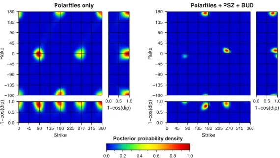
Polarities only Pol. + PSZ Pol. + BUD Pol. + PSZ + BUD

Iliny

2015−01−01 10:45

=3.9

PSZ BUD PSZ + BUD

M_L

Figure 11.Source mechanism solutions for the Iliny event (ML=3.9) derived by the proposed JOWAPO method using different data sets as indicated above the beach balls. For more details see the caption of Fig.2.

filter from 0.5 to 2 Hz to the observed displacement waveforms.

Both stations recorded simple seismograms with pronounced P- waves on the vertical components and distinctS-waves on the horizontal components, all suitable for further analysis (Fig.6). We carried out similar experiments as in the case of the Oroszl´any test event. The reference mechanism together with the results of the inverse calculations are listed in Table2and plotted in Fig.7.

Fig.7shows that the polarities only inversion resulted in a very poorly constrained mechanism. Even the 50 per cent confidence

zones are very large for both thePandTaxes. Consequently, the faulting style of the event can hardly be decided as well (pSS=0.33, pNF=0.18,pTF=0.17). The large areas of medium to high probability in the PPD plot also illustrate the very low reliability of the solution (Fig.8, left). Considering the small number of the polarities used in the inversion, this result is not surprising at all.

Including a single station in the inversion considerably decreased the uncertainties of the resulting focal mechanism, but the optimum solutions differ notably from the reference mechanism (Fig.7, first

(10)

−180

−135

−90

−45 0 45 90 135 180

Polarities only

Rake

0.0 0.5 1.0 1−cos(dip) 0.0

0.5 1.0

0 45 90 135 180 225 270 315 360 Strike

1−cos(dip)

−180

−135

−90

−45 0 45 90 135 180

Polarities + PSZ + BUD

Rake

0.0 0.5 1.0 1−cos(dip) 0.0

0.5 1.0

0 45 90 135 180 225 270 315 360 Strike

1−cos(dip)

0.0 0.2 0.4 0.6 0.8 1.0

Figure 12.Posterior probability density (PPD) of the source parameters for the Iliny event (ML=3.9). Left: PPD obtained by the proposed JOWAPO method using polarity data alone. Right: PPD derived using polarities and waveforms observed at two seismic stations, PSZ and BUD. The presented 2-D marginal probability densities are normalized individually.

d=37.2 c=0.79 vr=0.56 a=1804

PSZ_Z_P

d=37.2 c=0.94 vr=0.89 a=2347

PSZ_E_P

d=37.2 c=0.79 vr=0.61 a=1046

PSZ_N_P

d=67.2 c=0.88 vr=0.73 a=413

BUD_Z_P

0 s 6 s

d=67.2 c=0.96 vr=0.82 a=531

BUD_E_P

0 s 6 s

d=67.2 c=0.88 vr=0.77 a=759

BUD_N_P

Figure 13.Waveform comparison for the Iliny event (ML = 3.9). The observed seismograms (grey lines) are band-pass filtered with cut-off frequencies of 0.4 and 0.8 Hz. For more details see the caption of Fig.5.

row). The inversion of the PKS7 waveforms produced a moment magnitude of 3.04, remarkably greater than the reference magnitude of 2.73. The confidence regions of the principal axes are again somewhat larger for the more distant station PKS5 than for the nearest PKS7.

When using all the available data sets (polarities and waveforms at both stations), the JOWAPO inversion resulted in a satisfactory solution. It has high reliability and agrees very well with the reference mechanism (Table2). The directions of the principal axes are well defined (Fig.7) and the PPD has very small areas of high probability (Fig.8, right). The optimum solution is found at a source depth of 11 km, close to both the hypocentral depth of 12.2 km and the waveform inversion given depth of 13 km. The resulting moment magnitude of 2.77 also approximates well the reference magnitude.

The probability that the mechanism is SS is more than 0.99. Fig.9

illustrates that for short epicentral distances very good waveform fit can be achieved even at relatively high frequencies.

The optimum focal mechanisms produced by the waveform only inversions (Table2and Fig.7, second row) are similar to those obtained when polarities were also included in the calculations, but with somewhat larger uncertainties. The impact of the polarities on the solutions is, however, not so pronounced than in the case of the Oroszlány test event. It may be due to the fact that the number of the available polarity readings is much smaller for the Szabadszállás event than for the Oroszlány earthquake (5 versus 15). Nevertheless, for the single-station inversions, the beneficial effect of including polarities in the calculations is obvious.

At the end of this section we can conclude that if the number of the polarity data is large enough, even single-station JOWAPO inversion can produce usable focal mechanism solutions. However, for getting really reliable mechanisms, it is better to utilize more than one station in the inversion. When only a few polarities are available, single-station inversion may result in biased mechanisms.

In this case, using more than one station seems to be essential.

5 A P P L I C AT I O N I N N O RT H H U N G A RY Between 2013 June and 2015 January, 35 earthquakes with local magnitudeMLranging from 1.1 to 4.2 occurred in North Hungary.

W´eber (2016b) thoroughly investigated this earthquake sequence and successfully estimated the full moment tensors of fourML ≥ 3.4 events using long-period waveform inversion. Unfortunately, an additional earthquake near Iliny (Fig.1) withML3.9 could not be analysed at long periods because the observed waveforms had too low SNR at low frequencies. However, the JOWAPO method introduced in this paper offers an opportunity to estimate the focal mechanism of the Iliny event utilizing first motion polarities and short-period near-station seismograms.

For inversion, we considered the two nearest stations, PSZ and BUD, at epicentral distances of 37.2 and 67.2 km, respectively (Fig.1). At the time of the event, the stations were equipped with Streckeisen STS-2 broad-band seismometers with natural period of

(11)

SLOVAKIA HUNGARY

Balassagyarmat

Érsekvadkert

Szügy

Mohora

Cserhátsurány Nógrád−

marcal

Iliny

19.20˚E 19.20˚E

19.30˚E 19.30˚E

19.40˚E 19.40˚E

19.50˚E 19.50˚E

48.00˚N 48.00˚N

48.05˚N 48.05˚N

0 km 5 km

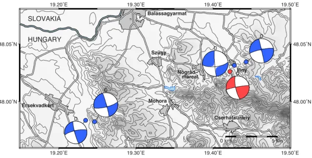
Figure 14.Optimum (maximum likelihood) source mechanism of the analysed Iliny earthquake (red) on a map of the source area. The mechanisms of four other events occurred in the same earthquake sequence (blue) are shown after W´eber (2016b). Beach ball size is proportional to event magnitude (shaded area:

compression; open area: dilatation). Equal area projection of lower hemisphere is used.

120 s. Since the epicentral distances of the selected stations are relatively large, the high-frequency content of the waveforms to be inverted should be kept at a minimum. On the other hand, the value of the lower cut-off frequency should be high enough to avoid the low SNR at long periods. Eventually, we applied a causal band-pass filter from 0.4 to 0.8 Hz to the observed displacement waveforms be- fore inversion. Due to the lack of well-identifiableS-waves, we used the initialP-wave trains of the recorded seismograms for analysing the event (Fig.10).

First, we estimated the focal mechanism of the Iliny earthquake utilizing only the 17 available P-wave polarities and accepting the hypocentral depth of 1.7 km derived from arrival times (Ta- ble1). The optimal JOWAPO solution is an SS event (Table2) with pSS=0.94. The reliability of the result is much better than that for the test events, but the uncertainty is still large (Figs11and12).

When inverting both waveforms and polarities, the optimum JOWAPO solutions differ only slightly from the polarity solution (Table2), but their reliability is considerably higher (Fig.11, first row). The most reliable solution was retrieved when both PSZ and BUD were included in the inverse calculations. The directions of both thePandTprincipal axes are well constrained (Fig.11) and the PPD has small areas of high probability (Fig.12). The optimum solution is found at a source depth of 4 km. It is very similar to the focal depths of 4 and 5 km obtained by W´eber (2016b) for two other earthquakes near Iliny applying a waveform inversion procedure. The resulting moment magnitude is 3.78, whereas the probability that the mechanism is SS is almost 1.0. The optimum waveform match is illustrated in Fig. 13. The achieved correla- tions and variance reduction values demonstrate that we obtained acceptable waveform fitting.

When using only waveforms (without polarities) in the inversion, the resulting focal mechanisms are very uncertain (Fig.11, second row). For the single-station inversions the obtained uncertainties are actually greater than those achieved for the polarities only solution.

It is also observable that the polarities affect the reliability of the results more considerably than in the case of the test events. It may be due to the fact that the longer-period waveforms used for the Iliny

event contain less information than the shorter-period seismograms applied for the test earthquakes.

Naturally, the focal mechanism obtained by jointly inverting the available polarity data and the waveforms at both PSZ and BUD is considered as the final solution for the Iliny event. Fig.14com- pares this optimum JOWAPO focal mechanism to those calculated by W´eber (2016b) for four other events in the same earthquake sequence. The newly obtained mechanism is very similar to the previously determined ones suggesting that the earthquakes were generated on the same fault system by the same stress field.

6 D I S C U S S I O N S A N D C O N C L U S I O N S Obtaining the focal mechanisms of small earthquakes using sparse data sets is a challenging task. In this paper we introduced and tested a new method that jointly inverts waveforms and polarity data following a probabilistic approach. The procedure called JOWAPO inversion maps the PPD of the model parameters and estimates the maximum likelihood DC mechanism, the optimal source depth and the scalar moment of the investigated event. The uncertainties of the solution are described by confidence regions. The procedure has been designed specifically for situations in which neither the available polarity data alone nor the well predictable near-station seismograms alone are sufficient to obtain reliable focal mechanism solutions for weak events.

We have demonstrated that including waveforms in the inversion considerably reduces the uncertainties of the usually poorly constrained polarity solutions. The proposed JOWAPO inversion performs best when using waveforms from at least two seismic stations.

If the number of the polarity data is large enough, even single-station JOWAPO inversion can produce usable solutions. When only a few polarities are available, however, single-station inversion may result in biased mechanisms. In this case some caution must be taken when interpreting the results.

We have successfully applied the proposed inversion method to an earthquake near Iliny, North Hungary. Since the seismograms of this earthquake were contaminated by high observational errors at