Least squares estimation for the subcritical Heston model based on continuous time observations

Least squares estimation for the subcritical Heston model based on continuous time observations

M´aty´as Barczy^∗,, Bal´azs Nyul^∗∗ and Gyula Pap^∗∗∗

* MTA-SZTE Analysis and Stochastics Research Group, Bolyai Institute, University of Szeged, Aradi v´ertan´uk tere 1, H–6720 Szeged, Hungary.

** Faculty of Informatics, University of Debrecen, Pf. 12, H–4010 Debrecen, Hungary.

*** Bolyai Institute, University of Szeged, Aradi v´ertan´uk tere 1, H–6720 Szeged, Hungary.

e–mails: barczy@math.u-szeged.hu (M. Barczy), nyul.balazs@inf.unideb.hu (B. Nyul), papgy@math.u-szeged.hu (G. Pap).

Corresponding author.

Abstract

We prove strong consistency and asymptotic normality of least squares estimators for the sub- critical Heston model based on continuous time observations. We also present some numerical illustrations of our results.

1 Introduction

Stochastic processes given by solutions to stochastic differential equations (SDEs) have been frequently applied in financial mathematics. So the theory and practice of stochastic analysis and statistical inference for such processes are important topics. In this note we consider such a model, namely the Heston model

(dY_t= (a−bY_t) dt+σ₁√

Y_tdW_t, dX_t= (α−βY_t) dt+σ₂√

Y_t %dW_t+p

1−%²dB_t

, t>0, (1.1)

where a >0, b, α, β∈R, σ₁ >0, σ₂ >0, %∈(−1,1), and (W_t, B_t)_t>0 is a 2-dimensional standard Wiener process, see Heston [14]. For interpretation of Y and X in financial mathematics, see, e.g., Hurn et al. [20, Section 4], here we only note that X_t is the logarithm of the asset price at time t and Yt its volatility for each t>0. The first coordinate process Y is called a Cox-Ingersoll-Ross (CIR) process (see Cox, Ingersoll and Ross [9]), square root process or Feller process.

Parameter estimation for the Heston model (1.1) has a long history, for a short survey of the most recent results, see, e.g., the introduction of Barczy and Pap [5]. The importance of the joint estimation of (a, b, α, β) and not only of (a, b) stems from the fact that X_t is the logarithm of the asset price at time t having high importance in finance. In fact, in Barczy and Pap [5], we investigated asymptotic properties of maximum likelihood estimator of (a, b, α, β) based on continuous time observations

2010 Mathematics Subject Classifications: 60H10, 91G70, 60F05, 62F12.

Key words and phrases: Heston model, least squares estimator, strong consistency, asymptotic normality

arXiv:1511.05948v3 [math.ST] 8 Aug 2018

(Xt)t∈[0,T], T >0. In Barczy et al. [6] we studied asymptotic behaviour of conditional least squares estimator of (a, b, α, β) based on discrete time observations (Yi, Xi), i = 1, . . . , n, starting the process from some known non-random initial value (y₀, x₀)∈(0,∞)×R. In this note we study least squares estimator (LSE) of (a, b, α, β) based on continuous time observations (Xt)t∈[0,T], T > 0, starting the process (Y, X) from some known initial value (Y₀, X₀) satisfying P(Y₀ ∈(0,∞)) = 1.

The investigation of the LSE of (a, b, α, β) based on continuous time observations (X_t)_t∈[0,T],T >0, is motivated by the fact that the LSEs of (a, b, α, β) based on appropriate discrete time observations converge in probability to the LSE of (a, b, α, β) based on continuous time observations (X_t)_t∈[0,T], T >0, see Proposition 3.1. We do not suppose that the process (Y_t)_t∈[0,T] is observed, since it can be determined using the observations (Xt)_t∈[0,T] and the initial value Y0, which follows by a slight modification of Remark 2.5 in Barczy and Pap [5] (replacing y₀ by Y₀). We do not estimate the parameters σ₁, σ₂ and %, since these parameters could —in principle, at least— be determined (rather than estimated) using the observations (Xt)_t∈[0,T] and the initial value Y0, see Barczy and Pap [5, Remark 2.6]. We investigate only the so-called subcritical case, i.e., when b >0, see Definition 2.3.

In Section 2 we recall some properties of the Heston model (1.1) such as the existence and unique- ness of a strong solution of the SDE (1.1), the form of conditional expectation of (Yt, Xt), t > 0, given the past of the process up to time s with s∈[0, t], a classification of the Heston model and the existence of a unique stationary distribution and ergodicity for the first coordinate process of the SDE (1.1). Section 3 is devoted to derive a LSE of (a, b, α, β) based on continuous time observations (X_t)_t∈[0,T], T >0, see Proposition 3.1. We note that Overbeck and Ryd´en [27, Theorems 3.5 and 3.6]

have already proved the strong consistency and asymptotic normality of the LSE of (a, b) based on continuous time observations (Yt)_t∈[0,T],T >0, in case of a subcritical CIR process Y with an initial value having distribution as the unique stationary distribution of the model. Overbeck and Ryd´en [27, page 433] also noted that (without providing a proof) their results are valid for an arbitrary initial distribution using some coupling argument. In Section 4 we prove strong consistency and asymptotic normality of the LSE of (a, b, α, β) introduced in Section 3, so our results for the Heston model (1.1) in Section 3 can be considered as generalizations of the corresponding ones in Overbeck and Ryd´en [27, Theorems 3.5 and 3.6] with the advantage that our proof is presented for an arbitrary initial value (Y₀, X₀) satisfying P(Y₀∈(0,∞)) = 1, without using any coupling argument. The covariance matrix of the limit normal distribution in question depends on the unknown parameters a and b as well, but somewhat surprisingly not on α and β. We point out that our proof of technique for deriving the asymptotic normality of the LSE in question is completely different from that of Overbeck and Ryd´en [27]. We use a limit theorem for continuous martingales (see, Theorem 2.6), while Overbeck and Ryd´en [27] use a limit theorem for ergodic processes due to Jacod and Shiryaev [21, Theorem VIII.3.79] and the so-called Delta method (see, e.g., Theorem 11.2.14 in Lehmann and Romano [24]).

We also remark that the approximation in probability of the LSE of (a, b, α, β) based on continuous time observations (X_t)_t∈[0,T], T > 0, given in Proposition 3.1 is not at all used for proving the asymptotic behaviour of the LSE in question as T → ∞ in Theorems 4.1 and 4.2. Further, we mention that the covariance matrix of the limit normal distribution in Theorem 3.6 in Overbeck and Ryd´en [27] is somewhat complicated, while, as a special case of our Theorem 4.2, it turns out that it can be written in a much simpler form by making a simple reparametrization of the SDE (1) in Overbeck and Ryd´en [27], estimating −b instead of b (with the notations of Overbeck and Ryd´en [27]), i.e., considering the SDE (1.1) and estimating b (with our notations), see Corollary 4.3. Section

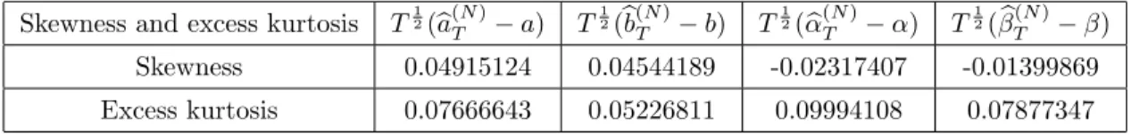
5 is devoted to present some numerical illustrations of our results in Section 4.

2 Preliminaires

Let N, Z+, R, R+, R++, R− and R−− denote the sets of positive integers, non-negative integers, real numbers, non-negative real numbers, positive real numbers, non-positive real numbers and negative real numbers, respectively. For x, y ∈R, we will use the notation x∧y:= min(x, y).

By kxk and kAk, we denote the Euclidean norm of a vector x∈R^d and the induced matrix norm of a matrix A∈R^d×d, respectively. By Id∈R^d×d, we denote thed-dimensional unit matrix.

Let Ω,F,P

be a probability space equipped with the augmented filtration (F_t)t∈R+ corre- sponding to (Wt, Bt)t∈R+ and a given initial value (η0, ζ0) being independent of (Wt, Bt)t∈R+ such that P(η₀ ∈R+) = 1, constructed as in Karatzas and Shreve [22, Section 5.2]. Note that (F_t)t∈R+

satisfies the usual conditions, i.e., the filtration (F_t)t∈R+ is right-continuous and F₀ contains all the P-null sets in F.

By C_c²(R+×R,R) and C_c^∞(R+×R,R), we denote the set of twice continuously differentiable real- valued functions on R+×R with compact support, and the set of infinitely differentiable real-valued functions on R+×R with compact support, respectively.

The next proposition is about the existence and uniqueness of a strong solution of the SDE (1.1), see, e.g., Barczy and Pap [5, Proposition 2.1].

2.1 Proposition. Let (η0, ζ0) be a random vector independent of (Wt, Bt)t∈R+ satisfying P(η0 ∈ R+) = 1. Then for all a∈R++, b, α, β ∈R, σ1, σ2 ∈R++, and %∈(−1,1), there is a pathwise unique strong solution (Y_t, X_t)t∈R+ of the SDE (1.1) such that P((Y₀, X₀) = (η₀, ζ₀)) = 1 and P(Yt∈R+ for all t∈R+) = 1. Further, for all s, t∈R+ with s6t,

(Y_t= e^−b(t−s)Y_s+aRt

se^−b(t−u)du+σ₁Rt

se^−b(t−u)√

Y_udW_u, X_t=X_s+Rt

s(α−βY_u) du+σ₂Rt s

√Y_ud(%W_u+p

1−%²B_u).

(2.1)

Next we present a result about the first moment and the conditional moment of (Yt, Xt)t∈R+, see Barczy et al. [6, Proposition 2.2].

2.2 Proposition. Let (Yt, Xt)t∈R+ be the unique strong solution of the SDE (1.1)satisfying P(Y0 ∈ R+) = 1 and E(Y₀)<∞, E(|X₀|)<∞. Then for all s, t∈R+ with s6t, we have

E(Y_t| F_s) = e^−b(t−s)Y_s+a Z t

s

e^−b(t−u)du, (2.2)

E(X_t| F_s) =X_s+ Z t

s

(α−βE(Y_u| F_s)) du (2.3)

=X_s+α(t−s)−βY_s Z t

s

e^−b(u−s)du−aβ Z t

s

Z u s

e^−b(u−v)dv

du, and hence

"

E(Y_t) E(X_t)

#

=

"

e^−bt 0

−βRt

e^−budu 1

# "

E(Y₀) E(X₀)

# +

" Rt

0e^−budu 0

−βRt Ru

e^−bvdv du t

# "

a α

# .

Consequently, if b∈R++, then

t→∞lim E(Y_t) = a

b, lim

t→∞t⁻¹E(X_t) =α−βa b , if b= 0, then

t→∞lim t⁻¹E(Yt) =a, lim

t→∞t⁻²E(Xt) =−1 2βa, if b∈R−−, then

t→∞lim e^btE(Y_t) =E(Y₀)−a

b, lim

t→∞e^btE(X_t) = β

b E(Y₀)−βa b².

Based on the asymptotic behavior of the expectations (E(Y_t),E(X_t)) as t → ∞, we recall a classification of the Heston process given by the SDE (1.1), see, Barczy and Pap [5, Definition 2.3].

2.3 Definition. Let (Yt, Xt)t∈R+ be the unique strong solution of the SDE (1.1) satisfying P(Y0 ∈ R+) = 1. We call (Yt, Xt)t∈R+ subcritical, critical or supercritical if b∈R++, b= 0 or b∈R−−, respectively.

In the sequel −→,^P −→^L and −→^a.s. will denote convergence in probability, in distribution and almost surely, respectively.

The following result states the existence of a unique stationary distribution and the ergodicity for the process (Y_t)t∈R+ given by the first equation in (1.1) in the subcritical case, see, e.g., Cox et al.

[9, Equation (20)], Li and Ma [25, Theorem 2.6] or Theorem 3.1 with α = 2 and Theorem 4.1 in Barczy et al. [4].

2.4 Theorem. Let a, b, σ1∈R++. Let (Yt)t∈R+ be the unique strong solution of the first equation of the SDE (1.1)satisfying P(Y₀∈R+) = 1. Then

(i) Yt

−→L Y∞ as t→ ∞, and the distribution of Y∞ is given by

E(e^−λY∞) =

1 +σ²₁ 2bλ

−2a/σ₁²

, λ∈R+, (2.4)

i.e., Y∞ has Gamma distribution with parameters 2a/σ²₁ and 2b/σ²₁, hence E(Y∞) = a

b, E(Y_∞²) = (2a+σ₁²)a

2b² , E(Y_∞³) = (2a+σ₁²)(a+σ₁²)a

2b³ .

(ii) supposing that the random initial value Y₀ has the same distribution as Y∞, the process (Yt)t∈R+ is strictly stationary.

(iii) for all Borel measurable functions f :R→R such that E(|f(Y_∞)|)<∞, we have

(2.5) 1

T Z T

0

f(Ys) ds−→^a.s. E(f(Y∞)) as T → ∞.

In what follows we recall some limit theorems for continuous (local) martingales. We will use these limit theorems later on for studying the asymptotic behaviour of least squares estimators of (a, b, α, β). First we recall a strong law of large numbers for continuous local martingales.

2.5 Theorem. (Liptser and Shiryaev [26, Lemma 17.4]) Let Ω,F,(F_t)t∈R+,P

be a filtered probability space satisfying the usual conditions. Let (Mt)t∈R+ be a square-integrable continuous local martingale with respect to the filtration (F_t)t∈R+ such that P(M₀ = 0) = 1. Let (ξ_t)t∈R+ be a progressively measurable process such that P Rt

0 ξ²_udhMi_u <∞

= 1, t∈R+, and Z t

0

ξ_u²dhMi_u−→ ∞^a.s. as t→ ∞, (2.6)

where (hMi_t)t∈R+ denotes the quadratic variation process of M. Then Rt

0ξ_udM_u Rt

0 ξ²_udhMi_u

−→a.s. 0 as t→ ∞.

(2.7)

If (Mt)t∈R+ is a standard Wiener process, the progressive measurability of (ξt)t∈R+ can be relaxed to measurability and adaptedness to the filtration (F_t)t∈R+.

The next theorem is about the asymptotic behaviour of continuous multivariate local martingales, see van Zanten [28, Theorem 4.1].

2.6 Theorem. (van Zanten [28, Theorem 4.1])Let Ω,F,(F_t)t∈R+,P

be a filtered probability space satisfying the usual conditions. Let (Mt)t∈R+ be a d-dimensional square-integrable continuous local martingale with respect to the filtration (F_t)t∈R+ such that P(M₀ = 0) = 1. Suppose that there exists a function Q:R+→R^d×d such that Q(t) is an invertible (non-random) matrix for all t∈R+, limt→∞kQ(t)k= 0 and

Q(t)hMi_tQ(t)^> −→^P ηη^> as t→ ∞,

where η is a d×drandom matrix. Then, for eachR^k-valued random vector v defined on (Ω,F,P), we have

(Q(t)M_t,v)−→^L (ηZ,v) as t→ ∞,

where Z is a d-dimensional standard normally distributed random vector independent of (η,v).

We note that Theorem 2.6 remains true if the function Q is defined only on an interval [t₀,∞) with some t0 ∈R++.

3 Existence of LSE based on continuous time observations

First, we define the LSE of (a, b, α, β) based on discrete time observations (Yⁱ

n, Xⁱ

n)i∈{0,1,...,bnTc}, n∈N, T ∈R++ (see (3.1)) by pointing out that the sum appearing in this definition of LSE can be considered as an approximation of the corresponding sum of the conditional LSE of (a, b, α, β) based on discrete time observations (Yⁱ

n, Xⁱ

n)i∈{0,1,...,bnTc}, n∈N, T ∈R++ (which was investigated in Barczy et al. [6]). Then we introduce the LSE of (a, b, α, β) based on continuous time observations (X_t)_t∈[0,T],T ∈R++ (see (3.4) and (3.5)) as the limit in probability of the LSE of (a, b, α, β) based on discrete time observations (Yⁱ

n, Xⁱ

n)i∈{0,1,...,bnTc}, n∈N, T ∈R++ (see Proposition 3.1).

A LSE of (a, b, α, β) based on discrete time observations (Yⁱ

n, Xⁱ

n)i∈{0,1,...,bnTc}, n∈N, T ∈R++, can be obtained by solving the extremum problem

ba^LSE,D_{T ,n} ,bb^LSE,D_T,n ,αb^LSE,D_{T ,n} ,βb_{T ,n}^LSE,D

:= arg min

(a,b,α,β)∈R⁴ bnTc

X

i=1

"

Yⁱ

n

−Yⁱ⁻¹

n

− 1 n

a−bYⁱ⁻¹

n

2

+

Xⁱ

n

−Xⁱ⁻¹

n

− 1 n

α−βYⁱ⁻¹

n

2# . (3.1)

Here in the notations the letter D refers to discrete time observations. This definition of LSE can be considered as the corresponding one given in Hu and Long [17, formula (1.2)] for generalized Ornstein-Uhlenbeck processes driven by α-stable motions, see also Hu and Long [18, formula (3.1)].

For a heuristic motivation of the LSE (3.1) based on the discrete observations, see, e.g., Hu and Long [16, page 178] (formulated for Langevin equations), and for a mathematical one, see as follows. By (2.2), for all i∈N,

Yⁱ

n

−E(Yⁱ

n

| Fi−1 n ) =Yⁱ

n

−e^−nbYⁱ⁻¹

n

−a Z ⁱ

n i−1

n

e^−b(ni−u)du=Yⁱ

n

−e^−nbYⁱ⁻¹

n

−a Z ¹

n

0

e^−bvdv

=





 Yⁱ

n

−Yⁱ⁻¹

n

−^a_n if b= 0, Yⁱ

n

−e^−nbYⁱ⁻¹

n +^a_b(e^−nb −1) if b6= 0.

Using first order Taylor approximation of e^−nb at b= 0 by 1− _n^b, and that of ^a_b(e^−nb −1) at (a, b) = (0,0) by −_n^a, the random variable Yi

n

−Yⁱ⁻¹

n

− ¹_n(a−bYⁱ⁻¹

n ) in the definition (3.1) of the LSE of (a, b, α, β) can be considered as a first order Taylor approximation of

Yi

n −E(Yi

n|Y₀, X₀, Y1 n, X1

n, . . . , Yⁱ⁻¹

n

, Xⁱ⁻¹

n

) =Yi

n −E(Yi n| Fⁱ⁻¹

n

),

which appears in the definition of the conditional LSE of (a, b, α, β) based on discrete time observa- tions (Yⁱ

n, Xⁱ

n)i∈{0,1,...,bnTc}, n∈N, T ∈R++. Similarly, by (2.3), for all i∈N, Xi

n

−E(Xi n

| Fi−1

n ) =Xi n

−Xⁱ⁻¹

n

−α

n +βYⁱ⁻¹

n

Z ⁱ

n i−1

n

e^{−b(u−i−1n} ) du+aβ Z ⁱ

n i−1

n

Z u

i−1 n

e^−b(u−v)dv

! du

=Xi n

−Xⁱ⁻¹

n

−α

n +βYⁱ⁻¹

n

Z _n¹

0

e^−budu+aβ Z ¹_n

0

Z u 0

e^−bvdv

du

=





 Xⁱ

n

−Xⁱ⁻¹

n

−^α_n+^β_nYⁱ⁻¹

n +_2n^aβ2 if b= 0,

Xi n

−Xⁱ⁻¹

n

−^α_n+^β_b(1−e^−nb)Yⁱ⁻¹

n + ^aβ_{b n}¹ −^1−e−

b n

b

if b6= 0.

Using first order Taylor approximation of _2n^aβ2 at (a, β) = (0,0) by 0, that of ^β_b(1−e^−nb) at (b, β) = (0,0) by ^β_n, and that of ^aβ_b ¹_n−^1−e−

nb

b

= ^aβ_n2

P∞

k=0(−1)^k(b/n)_(k+2)!^k at (a, b, β) = (0,0,0) by 0, the random variable Xi

n

−Xⁱ⁻¹

n

− ¹_n(α−βYⁱ⁻¹

n ) in the definition (3.1) of the LSE of (a, b, α, β) can be considered as a first order Taylor approximation of

Xi

n −E(Xi

n|Y₀, X₀, Y1 n, X1

n, . . . , Yⁱ⁻¹

n

, Xⁱ⁻¹

n

) =Xi

n −E(Xi n| Fⁱ⁻¹

n

),

which appears in the definition of the conditional LSE of (a, b, α, β) based on discrete time observa- tions (Yⁱ

n, Xⁱ

n)i∈{0,1,...,bnTc}, n∈N, T ∈R++.

We note that in Barczy et al. [6] we proved strong consistency and asymptotic normality of conditional LSE of (a, b, α, β) based on discrete time observations (Yi, Xi)i∈{1,...,n}, n∈N, starting the process from some known non-random initial value (y₀, x₀) ∈ R++×R, as the sample size n tends to infinity in the subcritical case.

Solving the extremum problem (3.1), we have

ba^LSE,D_{T ,n} ,bb^LSE,D_T,n

= arg min

(a,b)∈R² bnTc

X

i=1

Yi

n

−Yⁱ⁻¹

n

− 1 n

a−bYⁱ⁻¹

n

2

,

αb^LSE,D_{T ,n} ,βb_{T ,n}^LSE,D

= arg min

(α,β)∈R² bnTc

X

i=1

Xi

n

−Xⁱ⁻¹

n

− 1 n

α−βYⁱ⁻¹

n

2

,

hence, similarly as on page 675 in Barczy et al. [3], we get



 ba^LSE,D_{T ,n} bb^LSE,D_{T ,n}



=n





bnTc −PbnTc i=1 Yⁱ⁻¹

n

−PbnTc i=1 Yⁱ⁻¹

n

PbnTc i=1 Yi−1²

n





−1



Y^bnTc

n

−Y0

−PbnTc i=1 (Yi

n

−Yⁱ⁻¹

n

)Yⁱ⁻¹

n



, (3.2)

and



 αb^LSE,D_T,n βb_{T ,n}^LSE,D



=n





bnTc −PbnTc i=1 Yⁱ⁻¹

n

−PbnTc i=1 Yⁱ⁻¹

n

PbnTc i=1 Yi−1²

n





−1



XbnTc n

−X0

−PbnTc i=1 (Xi

n −Xⁱ⁻¹

n

)Yⁱ⁻¹

n



, (3.3)

provided that the inverse exists, i.e., bnTcPbnTc i=1 Yi−1²

n

>

PbnTc i=1 Yⁱ⁻¹

n

2

. By Lemma 3.1 in Barczy et al. [6], for all n ∈ N and T ∈ R++ with bnTc > 2, we have P

bnTcPbnTc i=1 Yi−1²

n

>

PbnTc i=1 Yⁱ⁻¹

n

2

= 1.

3.1 Proposition. If a∈R++, b∈R, α, β ∈R, σ₁, σ₂∈R++, ρ∈(−1,1), and P(Y₀∈R++) = 1, then for any T ∈R++, we have















 ba^LSE,D_{T ,n} bb^LSE,D_{T ,n} αb^LSE,D_T,n βb_{T ,n}^LSE,D

















−→P















 ba^LSE_T bb^LSE_T αb^LSE_T βb_T^LSE

















as n→ ∞,

where

"

ba^LSE_T bb^LSE_T

# :=

"

T −RT

0 Y_sds

−RT

0 Y_sds RT 0 Y_s²ds

#⁻¹"

Y_T −Y₀

−RT 0 Y_sdY_s

#

= 1

TRT

0 Y_s²ds− RT

0 Y_sds2

"

(Y_T −Y₀)RT

0 Y_s²ds−RT

0 Y_sdsRT 0 Y_sdY_s (Y_T −Y0)R_T

0 Ysds−TR_T

0 YsdYs

# , (3.4)

and

"

αb^LSE_T βb_T^LSE

# :=

"

T −RT

0 Y_sds

−RT

0 Y_sds RT 0 Y_s²ds

#⁻¹"

X_T −X₀

−RT

0 Y_sdX_s

#

= 1

TRT

0 Y_s²ds− RT

0 Y_sds2

"

(X_T −X₀)RT

0 Y_s²ds−RT

0 Y_sdsRT

0 Y_sdX_s (X_T −X₀)RT

0 Y_sds−TRT

0 Y_sdX_s

# , (3.5)

which exist almost surely, since

P T Z _T

0

Y_s²ds >

Z T 0

Y_sds ²!

= 1 for all T ∈R++. (3.6)

By definition, we call ba^LSE_T ,bb^LSE_T ,αb^LSE_T ,βb_T^LSE

the LSE of (a, b, α, β) based on continuous time observations (Xt)_t∈[0,T], T ∈R++.

Proof. First, we check (3.6). Note that P(RT

0 Ysds < ∞) = 1 and P(RT

0 Y_s²ds < ∞) = 1 for all T ∈R+, since Y has continuous trajectories almost surely. For each T ∈R++, put

A_T :={ω ∈Ω :t7→Yt(ω) is continuous and non-negative on [0, T]}.

Then AT ∈ F, P(AT) = 1, and for all ω ∈AT, by the Cauchy–Schwarz’s inequality, we have T

Z T 0

Y_s(ω)²ds>

Z T 0

Y_s(ω) ds 2

,

and TRT

0 Ys(ω)²ds− RT

0 Ys(ω) ds 2

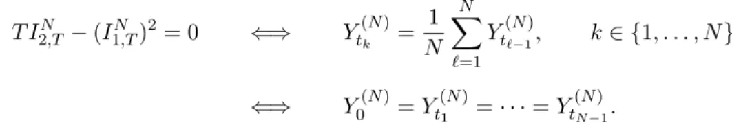
= 0 if and only if Ys(ω) = KT(ω) for almost every s ∈ [0, T] with some K_T(ω) ∈ R+. Hence Y_s(ω) = Y₀(ω) for all s ∈ [0, T] if ω ∈ A_T and TRT

0 Y_s²(ω) ds− RT

0 Ys(ω) ds 2

= 0. Consequently, using that P(AT) = 1, we have

P T Z T

0

Y_s²ds− Z T

0

Ysds 2

= 0

!

=P (

T Z T

0

Y_s²ds− Z T

0

Ysds 2

= 0 )

∩AT

!

6P(Y_s=Y₀, ∀s∈[0, T])6P(Y_T =Y₀) = 0,

where the last equality follows by the fact that YT is absolutely continuous (see, e.g., Alfonsi [2, Proposition 1.2.11]) together with the law of total probability. Hence P

TRT

0 Y_s²ds− RT

0 Y_sds2

= 0

= 0, yielding (3.6).

Further, we have 1

n





bnTc −PbnTc i=1 Yⁱ⁻¹

n

−PbnTc i=1 Yⁱ⁻¹

n

PbnTc i=1 Yi−1²

n





−→a.s.

"

T −RT

0 Y_sds

−R_T

0 Ysds R_T

0 Y_s²ds

#

as n→ ∞,

since (Y_t)t∈R+ is almost surely continuous. By Proposition I.4.44 in Jacod and Shiryaev [21] with the Riemann sequence of deterministic subdivisions _nⁱ ∧T

i∈N, n∈N, and using the almost sure

continuity of (Yt, Xt)t∈R+, we obtain





Y^bnTc

n

−Y0

−PbnTc i=1 (Yi

n

−Yⁱ⁻¹

n

)Yⁱ⁻¹

n





−→P

"

YT −Y0

−RT 0 Y_sdY_s

#

as n→ ∞,





XbnTc n

−X₀

−PbnTc i=1 (Xⁱ

n

−Xⁱ⁻¹

n )Yⁱ⁻¹

n





−→P

"

X_T −X₀

−RT

0 Y_sdX_s

#

as n→ ∞.

By Slutsky’s lemma, using also (3.2), (3.3) and (3.6), we obtain the assertion. 2 Note that Proposition 3.1 is valid for all b∈R, i.e., not only for subcritical Heston models.

We call the attention that (ba^LSE_T ,bb^LSE_T ,αb_T^LSE,βb_T^LSE) can be considered to be based only on (X_t)_t∈[0,T], since the process (Y_t)_t∈[0,T] can be determined using the observations (X_t)_t∈[0,T] and the initial value Y0, see Barczy and Pap [5, Remark 2.5]. We also point out that Overbeck and Ryd´en [27, formulae (22) and (23)] have already come up with the definition of LSE (ba^LSE_T ,bb^LSE_T ) of (a, b) based on continuous time observations (Y_t)_t∈[0,T], T ∈ R++, for the CIR process Y. They investigated only the CIR process Y, so our definitions (3.4) and (3.5) can be considered as generalizations of formulae (22) and (23) in Overbeck and Ryd´en [27] for the Heston model (1.1).

Overbeck and Ryd´en [27, Theorem 3.4] also proved that the LSE of (a, b) based on continuous time observations can be approximated in probability by conditional LSEs of (a, b) based on appropriate discrete time observations.

In the next remark we point out that the LSE of (a, b, α, β) given in (3.4) and (3.5) can be ap- proximated using discrete time observations for X, which can be reassuring for practical applications, where data in continuous record is not available.

3.2 Remark. The stochastic integral RT

0 Y_sdY_s in (3.4) is a measurable function of (X_s)_s∈[0,T]

and Y₀. Indeed, for all t ∈ [0, T], Y_t and Rt

0 Y_sds are measurable functions of (X_s)_s∈[0,T]

and Y0, i.e., they can be determined from a sample (Xs)s∈[0,T] and Y0 following from a slight modification of Remark 2.5 in Barczy and Pap [5] (replacing y₀ by Y₀), and, by Itˆo’s formula, we have d(Y_t²) = 2Y_tdY_t+σ₁²Y_tdt, t ∈ R+, implying that RT

0 Y_sdY_s = ¹₂ Y_T²−Y₀²−σ₁²RT 0 Y_sds

, T ∈R+. For the stochastic integral RT

0 Y_sdX_s in (3.5), we have (3.7)

bnTc

X

i=1

Yⁱ⁻¹

n (Xⁱ

n

−Xⁱ⁻¹

n )−→^P Z T

0

YsdXs as n→ ∞,

following from Proposition I.4.44 in Jacod and Shiryaev [21] with the Riemann sequence of determinis- tic subdivisions _nⁱ ∧T

i∈N, n∈N. Thus, there exists a measurable function Φ :C([0, T],R)×R→R such that RT

0 YsdXs= Φ((Xs)s∈[0,T], Y0), since the convergence in (3.7) holds almost surely along a suitable subsequence, for each n∈N, the members of the sequence in (3.7) are measurable functions of (X_s)_s∈[0,T] and Y₀, and one can use Theorems 4.2.2 and 4.2.8 in Dudley [13]. Hence the right hand sides of (3.4) and (3.5) are measurable functions of (Xs)_s∈[0,T] and Y0, i.e., they are statistics.

2

Using the SDE (1.1) and Corollary 3.2.20 in Karatzas and Shreve [22], one can check that

"

ba^LSE_T −a bb^LSE_T −b

#

=

"

T −RT

0 Y_sds

−RT

0 Ysds RT 0 Y_s²ds

#⁻¹"

σ₁RT

0 Ys^1/2dW_s

−σ₁RT

0 Ys^3/2dWs

# ,

"

αb^LSE_T −α βb_T^LSE−β

#

=

"

T −R_T

0 Ysds

−RT

0 Ysds RT 0 Y_s²ds

#⁻¹"

σ2

R_T

0 Ys^1/2dWfs

−σ₂RT

0 Ys^3/2dWfs

# ,

provided that TRT

0 Y_s²ds >

RT

0 Y_sds2

, where fW_t:=%W_t+p

1−%²B_t, t∈R+, and hence

ba^LSE_T −a= σ₁

RT

0 Ys^1/2dW_s RT

0 Y_s²ds

−σ₁ RT

0 Y_sds RT

0 Ys^3/2dW_s TRT

0 Y_s²ds− RT

0 Y_sds2 ,

bb^LSE_T −b= σ₁

RT

0 Ys^1/2dW_s RT

0 Y_sds

−σ₁TRT

0 Ys^3/2dW_s TRT

0 Y_s²ds− RT

0 Y_sds2 ,

αb^LSE_T −α= σ2

RT

0 Ys^1/2dWfs

RT 0 Y_s²ds

−σ2

RT

0 Ysds RT

0 Ys^3/2dWfs

TRT

0 Y_s²ds− RT

0 Ysds

2 ,

βb_T^LSE−β = σ₂

RT

0 Y_s^1/2dfW_s RT

0 Y_sds

−σ₂TRT

0 Y_s^3/2dfW_s TRT

0 Y_s²ds− RT

0 Y_sds2 ,

(3.8)

provided that TRT

0 Y_s²ds >

RT

0 Y_sds2

.

4 Consistency and asymptotic normality of LSE

Our first result is about the consistency of LSE in case of subcritical Heston models.

4.1 Theorem. If a, b, σ1, σ2 ∈ R++, α, β ∈ R, % ∈ (−1,1), and P((Y0, X0) ∈ R++×R) = 1, then the LSE of (a, b, α, β) is strongly consistent, i.e., ba^LSE_T ,bb^LSE_T ,αb^LSE_T ,βb_T^LSE a.s.

−→ (a, b, α, β) as T → ∞.

Proof. By Proposition 3.1, there exists a unique LSE ba^LSE_T ,bb^LSE_T ,αb^LSE_T ,βb_T^LSE

of (a, b, α, β) for all T ∈R++. By (3.8), we have

ba^LSE_T −a=

σ₁·_T¹ RT

0 Y_sds·_T¹ RT

0 Y_s²ds·

RT

0 Ys^1/2dWs

RT

0 Ysds −σ₁·_T¹ RT

0 Y_sds·_T¹ RT

0 Y_s³ds·

RT

0 Ys^3/2dWs

RT 0 Y_s³ds 1

T

RT

0 Y_s²ds−

1 T

RT 0 Ysds

2

provided that RT

0 Ysds∈R++, which holds almost surely, see the proof of Proposition 3.1. Since, by part (i) of Theorem 2.4, E(Y∞), E(Y_∞²),E(Y_∞³)∈R++, part (iii) of Theorem 2.4 yields

1 T

Z T 0

Ysds−→^a.s. E(Y∞), 1 T

Z T 0

Y_s²ds−→^a.s. E(Y_∞²), 1 T

Z T 0

Y_s³ds−→^a.s. E(Y_∞³)

as T → ∞, and then Z T

0

Y_sds−→ ∞,^a.s.

Z T 0

Y_s²ds−→ ∞,^a.s.

Z T 0

Y_s³ds−→ ∞^a.s.

as T → ∞. Hence, by a strong law of large numbers for continuous local martingales (see, e.g., Theorem 2.5), we obtain

ba^LSE_T −a−→^a.s. σ₁·E(Y∞)·E(Y_∞²)·0−σ₁·E(Y∞)·E(Y_∞³)·0

E(Y_∞²)−(E(Y∞))² = 0 as T → ∞, where for the last step we also used that E(Y_∞²)−(E(Y∞))² = ^aσ_2b2²¹ ∈R++.

Similarly, by (3.8),

bb^LSE_T −b= σ₁·

1 T

RT

0 Y_sds2

·

RT

0 Ys^1/2dWs

RT

0 Ysds −σ₁·_T¹ RT

0 Y_s³ds·

RT

0 Ys^3/2dWs

RT 0 Y_s³ds 1

T

RT

0 Y_s²ds−

1 T

RT

0 Y_sds2

−→a.s. σ1·(E(Y∞))²·0−σ1·E(Y_∞³)·0

E(Y_∞²)−(E(Y∞))² = 0 as T → ∞.

One can prove

αb^LSE_T −α−→^a.s. 0 and βb_T^LSE−β −→^a.s. 0 as T → ∞

in a similar way. 2

Our next result is about the asymptotic normality of LSE in case of subcritical Heston models.

4.2 Theorem. If a, b, σ1, σ2 ∈R++, α, β ∈R, %∈(−1,1) and P((Y0, X0)∈R++×R) = 1, then the LSE of (a, b, α, β) is asymptotically normal, i.e.,

T¹²















ba^LSE_T −a bb^LSE_T −b αb^LSE_T −α βb^LSE_T −β















−→ NL ₄



0,S⊗





(2a+σ²₁)a σ₁²b

2a+σ²₁ σ₁² 2a+σ₁²

σ²₁

2b(a+σ₁²) σ²₁a







 as T → ∞, (4.1)

where ⊗ denotes the tensor product of matrices, and

S :=

"

σ₁² %σ1σ2

%σ1σ2 σ²₂

# .

With a random scaling, we have

E⁻

1 2

1,T I₂⊗





(T E_2,T −E_1,T² ) E_1,TE_3,T −E_2,T² −¹₂

0

−T E_1,T



















ba^LSE_T −a bb^LSE_T −b αb^LSE_T −α βb_T^LSE−β















−→ NL ₄(0,S⊗I₂) (4.2)

→ ∞, where RT i ∈

Proof. By Proposition 3.1, there exists a unique LSE ba^LSE_T ,bb^LSE_T ,αb^LSE_T ,βb_T^LSE

of (a, b, α, β). By (3.8), we have

√

T(ba^LSE_T −a) =

1 T

RT

0 Y_s²ds ·^√σ1

T

RT

0 Ys^1/2dW_s−_T¹ RT

0 Y_sds ·^√σ1

T

RT

0 Ys^3/2dW_s

1 T

RT

0 Y_s²ds−

1 T

RT 0 Ysds

2 ,

√

T(bb^LSE_T −b) =

1 T

RT

0 Y_sds ·^√σ1

T

RT

0 Y_s^1/2dW_s−^√σ1

T

RT

0 Y_s^3/2dW_s

1 T

RT

0 Y_s²ds−

1 T

RT

0 Y_sds2 ,

√

T(αb^LSE_T −α) =

1 T

RT

0 Y_s²ds ·^√σ2

T

RT

0 Ys^1/2dfWs−_T¹ RT

0 Ysds ·^√σ2

T

RT

0 Ys^3/2dWfs 1

T

RT

0 Y_s²ds−

1 T

RT

0 Y_sds2 ,

√

T(βb^LSE_T −β) =

1 T

RT

0 Ysds ·^√σ2

T

RT

0 Ys^1/2dWfs−^√σ2

T

RT

0 Ys^3/2dWfs 1

T

RT

0 Y_s²ds−

1 T

RT 0 Ysds

2 ,

provided that TRT

0 Y_s²ds >

RT

0 Y_sds2

, which holds almost surely. Consequently,

√ T















ba^LSE_T −a bb^LSE_T −b αb^LSE_T −α βb_T^LSE−β















= 1

1 T

RT

0 Y_s²ds−

1 T

RT 0 Ysds

2 I2⊗

"₁

T

RT

0 Y_s²ds _T¹ RT 0 Y_sds

1 T

RT

0 Y_sds 1

#!

√1 TMT

=



I2⊗

"

1 −_T¹ RT 0 Ysds

−_T¹ RT

0 Y_sds _T¹ RT 0 Y_s²ds

#⁻¹



√1 TMT, (4.3)

provided that TRT

0 Y_s²ds >

RT

0 Y_sds2

, which holds almost surely, where

Mt:=















 σ₁Rt

0Ys^1/2dW_s

−σ₁Rt

0Ys^3/2dW_s σ₂Rt

0Y_s^1/2dfW_s

−σ₂Rt

0Y_s^3/2dfW_s

















, t∈R+,

is a 4-dimensional square-integrable continuous local martingale due to Rt

0E(Ys) ds < ∞ and Rt

0 E(Y_s³) ds <∞,t∈R+. Next, we show that

√1

TM_T −→^L ηZ as T → ∞, (4.4)

where Z is a 4-dimensional standard normally distributed random vector and η∈R^4×4 such that ηη^>=S⊗

"

E(Y∞) −E(Y_∞²)

−E(Y_∞²) E(Y_∞³)

# .