E F F I C I E N T M AT R I X - A N A LY T I C S O L U T I O N O F M U L T I -T Y P E Q U E U E I N G S Y S T E M S W I T H C O R R E L AT E D T R A F F I C
gábor horváth
Dissertation submitted to the Hungarian Academy of Sciences for the degree of Doctor of Sciences
2017, Budapest
A B S T R A C T
Erlang defined and solved the first queueing model 100 years ago to characterize the number of active calls in a telephone exchange. Since then, queueing theory has been an essential tool in the research of telecommunication systems.
The application of classical queueing models for the analysis of modern telecommunication networks is increasingly challenging: both the stochastic behavior of the traffic and the sched- ulers forwarding the packets in the network devices are becoming more and more complex.
The so-called matrix-analytic methods allow to solve many of the corresponding complex queueing systems efficiently, with Markovian tools. This dissertation provides an overview on these modern techniques of queueing theory and presents several new results.
In the first part the main tools of the Markovian workload characterization, the phase-type distributions and the Markovian arrival processes are considered. For both traffic models, the role of the representations is discussed, special representations are introduced and new moment matching methods are developed. These results make it possible to create Markovian models for the network traffic, that can be used both in simulation based and in analytical performance analysis.
The second part of the dissertation presents the solution of single-class and multi-class queues with correlated arrival processes and Markovian service times. In the multi-class case both the first-come-first-served and the priority service policy are considered. Many performance measures are derived based on the analysis of the queue length process, the workload process and the age process. The characteristics of the traffic departing from these queues are also investigated.
In the third part a novel queueing network solution approach is described, that integrates the results of the first two parts. In this approach the traffic of the queueing network is characterized by Markovian arrival processes discussed in the first part, and the nodes of the network are the queues discussed in the second part of the dissertation. The Markovian arrival processes representing the internal traffic are obtained by moment matching. An extensive numerical study investigates the behavior of the presented approach and compares it with other existing solutions from the literature.
A C K N O W L E D G M E N T S
There are many people to whom I am grateful for their contribution to the results presented in this dissertation, it is impossible to list everyone. Let me mention only a couple of them. At the first place I would like to thank my family for their patience. I have to thank the Department of Networked Systems and Services for providing the flexibility and the intellectual freedom in my work. Last but not least, to Miklós Telek for the pleasant common work and for the many valuable advice and encouragement in both personal and scientific questions.
C O N T E N T S
1 introduction 1
1.1 Motivation . . . 1
1.1.1 Queueing theory for analyzing computer and communication systems 1 1.1.2 Further application fields of queueing theory . . . 2
1.2 Markovian performance analysis . . . 2
1.2.1 Workload models . . . 3
1.2.2 Queues . . . 5
1.2.3 Queueing networks . . . 6
1.3 The structure of the dissertation . . . 7
I workload modeling 9 2 phase-type distributions 11 2.1 Introduction to Phase-Type distributions . . . 11
2.1.1 Matrix-exponential distributions . . . 11
2.1.2 Representation transformations . . . 12
2.1.3 Phase-type distributions . . . 14
2.1.4 Important representations . . . 14
2.2 Canonical forms . . . 17
2.2.1 Canonical representation of PH(2) distributions . . . 18
2.2.2 Canonical representation of PH(3) distributions . . . 19
2.2.3 Canonical representation of PH(4) distributions . . . 23
2.3 PH fitting with canonical forms . . . 24
2.3.1 Moment matching . . . 25
2.3.2 Fitting the density function . . . 26
2.4 PH fitting with a flexible structure . . . 28
2.4.1 Solution of the moment matching problem with fixedri parameters . . 29
2.4.2 Optimizing theriparameters . . . 29
2.4.3 Numerical examples . . . 31
3 markovian arrival processes 37 3.1 Introduction to Markovian arrival processes . . . 37
3.1.1 Definition and basic properties . . . 37
3.1.2 Marked Markovian arrival processes . . . 39
3.1.3 Representation transformation . . . 41
3.2 Minimal characterization of MMAPs and a moment matching method . . . 42
3.2.1 Minimal characterization of single-type RAPs . . . 42
3.2.2 A moment matching method . . . 43
3.2.3 Extension to the multi-type case . . . 44
3.2.4 Obtaining Markovian representation with successive transformations 46 3.3 Obtaining an approximate Markovian representation . . . 48
3.3.1 The two-step fitting approach . . . 48
3.3.2 Fitting the distribution of the inter-arrival times . . . 48 3.3.3 Approximate Markovian representation by fitting the joint moments . 49 3.3.4 Approximate Markovian representation by fitting the joint distribution 53
viii contents
II qeues 59
4 skip-free processes 61
4.1 Quasi Birth-Death Processes . . . 61
4.1.1 Simple birth-death processes . . . 61
4.1.2 Quasi birth-death processes . . . 62
4.1.3 Stationary solution of QBDs . . . 63
4.1.4 Busy period analysis . . . 64
4.2 Markovian Fluid Models . . . 65
4.2.1 Model definition . . . 65
4.2.2 Stationary solution . . . 65
4.2.3 Busy period analysis of Markovian fluid models . . . 67
5 analysis of the map/map/1 qeue 71 5.1 Analysis of the number of customers in the system . . . 71
5.2 Sojourn time analysis . . . 72
5.2.1 Sojourn time analysis based on the age process . . . 73
5.2.2 Sojourn time analysis based on the workload process . . . 75
5.3 Departure process analysis . . . 76
5.3.1 Level probability based truncation method . . . 77
5.3.2 ETAQA truncation method . . . 78
5.3.3 Joint moment based departure process approximation . . . 78
6 analysis of the mmap[k]/ph[k]/1-fcfs qeue 83 6.1 The distribution of the age process . . . 83
6.2 Deriving the sojourn time from the age process . . . 85
6.3 Analysis of the number of customers . . . 85
6.4 Analysis of the departure process . . . 87
6.4.1 Distribution of the age process at departure instants . . . 87
6.4.2 Phase transitions over the busy period of the age process . . . 87
6.4.3 The lag-njoint transform of the departure process . . . 87
6.4.4 The inter-departure time distribution and lag-1joint moments . . . 92
7 analysis of the mmap[k]/ph[k]/1 priority qeue 97 7.1 Analysis of the preemptive resume priority queue . . . 97
7.1.1 The workload of the system just after low priority arrival instants . . . 98
7.1.2 The sojourn time of low priority customers . . . 100
7.1.3 Number of low priority customers in the system . . . 101
7.1.4 The analysis of the high priority class . . . 104
7.2 Analysis of the non-preemptive priority queue . . . 104
7.2.1 The workload of the system just before low priority arrival instants . . 104
7.2.2 The sojourn time of low priority customers . . . 105
7.2.3 The number of low priority customers . . . 107
7.2.4 The analysis of the high priority class . . . 108
7.3 Numerical behavior . . . 112
7.4 Departure process analysis of priority queues . . . 112
7.4.1 The MMAP[K]/PH[K]/1 preemptive priority queue as a QBD process . 113 7.4.2 Analysis of level zero . . . 116
7.4.3 The joint moments of the departure process . . . 117
7.4.4 An efficient, truncation-free procedure . . . 119
contents ix
III qeueing networks 127
8 qeueing network analysis based on the joint moments 129
8.1 Traffic based decomposition for the analysis of queueing networks . . . 129
8.2 Single-type queueing networks . . . 130
8.2.1 MAP based approximations for the departure process . . . 130
8.2.2 Numerical results with a tandem network . . . 132
8.2.3 A more complex numerical example . . . 136
8.2.4 Summary of the single-type results . . . 136
8.3 Multi-type queueing networks . . . 138
8.3.1 Studying the effect of the service discipline . . . 138
8.3.2 A two-node tandem network . . . 140
8.3.3 The more complex example with two customer types . . . 141
8.3.4 Summary of the multi-type results . . . 142
9 concluding remarks and future work 145 10 summary 147 IV appendix 151 a fundamental relations 153 a.1 Kronecker operations . . . 153
a.2 Properties of the matrix-exponential function . . . 155
b proofs of theorems 157 b.1 Proof of Lemma1 . . . 157
b.2 Proof of Theorem7 . . . 158
A C R O N Y M S
CTMC continuous time Markov chain DTMC discrete time Markov chain PH phase-type
ME matrix-exponential FEB feedback Erlang block MAP Markovian arrival process
MMAP marked Markovian arrival process
SMMAP structured marked Markovian arrival process SMAP structured Markovian arrival process
RAP rational arrival process
MRAP marked rational arrival process QBD quasi birth-death process MFM Markovian fluid model LST Laplace-Stieltjes transform GF generating function
SCV squared coefficient of variation
NARE non-symmetric algebraic Riccati equation FCFS first-come-first-served
pdf probability density function cdf cumulative distribution function iid. independent and identically distributed
N O TAT I O N S
I Identity matrix of appropriate size
1 Column vector of ones of appropriate size
L(t) The level process of QBDs and Markovian fluid models at timet J(t) The phase process at timet
C(t) The type of the customer in the server at timet
N The number of phases
π The (row) vector of stationary probabilities π(x) The (row) vector of stationary densities
X The stationary number of customers in the system at departure instants Y The stationary number of customers in the system at random instants
A(t) The age process
V(t) The workload process
B The busy period
T The stationary sojourn time of customers W The stationary waiting time of customers
D0,D1 The matrices characterizing the MAP of the arrivals
S,(Sk) The random variable representing the (typek) service times σ,S The parameters of the PH distributed service times
S0,S1 The matrices characterizing the MAP of the service times H The random variable representing the inter-departure times H0,H1 The matrices characterizing the MAP of the departures Q The generator matrix of a continuous time Markov chain θ The stationary phase distribution of the background process
1
I N T R O D U C T I O N
1.1 motivation
1.1.1 Queueing theory for analyzing computer and communication systems
The application of queueing theory in the field of telecommunication has a long history.
At the beginning of the last century, the wide spread deployment of plain old telephone systems established the need for efficient dimensioning methods. The goal was to determine the number of trunks required to meat a certain level of service quality. Erlang was the first to model the number of active calls with a queueing system. He proved that the telephone traffic can be modeled by a Poisson process and created the classic formulas for call loss and waiting time. This was the first engineering problem that was solved by queueing theory.
Over time, newer and newer telecommunication technologies have been developed. With the appearance of data traffic the packet switched communication method started to gain pop- ularity, packet based technologies like the ATM (Asynchronous Transfer Mode) and the IP (In- ternet Protocol) have slowly superseded the circuit switched technology. The packet switched networking gave an other boost to the application of queueing models in telecommunica- tion. Since the quality of service (QoS) measures like packet loss and delay are associated with the buffers in the network nodes (where packets are residing temporarily before get- ting forwarded to the next node), open queueing networks appeared to be the ideal modeling tools for performance analysis [32,15].
Compared to the detailed simulation of the system, the analytical solution of queueing mod- els usually need less input data (hence easier to use) and is usually very fast. Consequently, it enables the fast evaluation of different possibilities for providing service, performing param- eter sensitivity analysis, or just to gain insight into the behavior of the system.
Modern telecommunication systems, however, have some unique properties that make the application of queueing models increasingly challenging. Some of the reasons are listed below.
• The characteristic of the traffic has changed considerably in the recent decades. While the Poisson process is still a reasonable model for voice call arrivals, the data traffic be- haves differently. Statistical properties like long-term correlations, self-similar behav- ior and heavy tailed distributions make the direct application of the classical queueing models difficult [38].
• The network traffic is grouped into various classes according to the quality demands.
While there are some basic queueing models available that support such traffic differ- entiation, more general queueing models are substantially more difficult to solve in the multi-class case.
2 introduction
• Communication technologies are becoming very complex: the underlying protocols have multiple interacting layers, and use several (possibly interfering) flow control al- gorithms. It is becoming increasingly difficult to identify the components of the system that have the dominant impact on the overall performance. Analytical models for such complex systems have to introduce many assumptions and simplifications.
Looking for answers for these challenges has been the main driver of queueing theory re- search in the recent years.
1.1.2 Further application fields of queueing theory
Although the modeling of telecommunication systems is still the most popular application area of queueing theory, there are several other fields where queueing models are used fre- quently.
One of these emerging application fields ishealthcare ([31]), where queueing systems are applied to optimize the cost by minimizing the inefficiencies and delays. In a healthcare pro- cess the demands waiting in the queue are the patients, and the servers are the doctors or any other specialized equipment (like an operating room). Compared to telecommunication sys- tems, queues in healthcare have some specialties, including that
• patients are impatient,
• the arrival rate is varying and depends on the state of the system (patients do not join the waiting line when it is too long),
• the service discipline is more complex.
Queueing models can be used for health care system design (to determine the optimal num- ber of beds, ambulance cars, etc.), for health care operation (for the optimal scheduling of resources, patients, appointments, bed and staff management, etc.) and also in health care system analysis (to calculate the utilization, cost, delays, etc.) [55].
Queueing network models are used in the design and analysis of manufacturing systems since the 1950s as well ([34]). In a manufacturing system there are resources (machines), which perform various processing steps on products. From queueing point of view the cus- tomers are the parts, which, after arriving into the queue, have to wait till the suitable ma- chines (that are the servers in queueing terminology) become available. Both the arrival pro- cess and the processing times are stochastic. A manufacturing system typically consists of many processing stations with their own buffers for the parts, and the parts have to go through many processing stations to become a final product. Hence, a queueing network model is a natural choice both for performance evaluation and optimization purposes, thus to analyze or optimize the material flow in the system, the utilization of the machines, the capacity of the buffers, etc.
Apart of these two application fields, queueing models have been successfully applied in many other areas as well, including vehicular traffic analysis [4], inventory systems [35], housing [52], banking [29], or even to optimize crowd sourcing systems [24].
1.2 markovian performance analysis
The solution of many tractable queueing models is based on the analysis of a closely related Markov chain.
1.2 markovian performance analysis 3 The queue length of basic queues having memoryless inter-arrival and service times (in- cluding the M/M/1, M/M/m, M/M/m/m queues [53], etc.) can be represented by a Markov chain directly, that, due to the regular tri-diagonal structure of the generator has a simple and explicit stationary solution, even for infinite systems.
The analysis of more complex queueing systems, were either the arrival or the service times are generally distributed, is based on the solution of an appropriately defined Markov chain as well. In case of G/M/1 (M/G/1) systems the Markov chain characterizing the queue length at specific embedded time instants has an upper Hessenberg (lower Hessenberg) structure, respectively. The regular structure enables the efficient solution of these systems.
Starting from the eighties, Markovian performance modeling has undergone an enormous development. The introduction of phase-type distributions and Markovian arrival processes made it possible to characterize a reasonably general class of arrival and service processes in a Markovian way. The generators of the Markov chains describing the related queues also have a regular structure, at block level. An elegant, numerically efficient solution methodology has been developed to solve such block-structured Markov chains, calledmatrix-analytic method ([65,57]), which became one of the cornerstones of modern queueing theory.
The results derived in this dissertation rely on matrix-analytic methods heavily.
1.2.1 Workload models
To obtain relevant, meaningful results from a queueing model the workload must be char- acterized as accurately as possible. The workload characterization has two ingredients: the characterization of the arrival process of the demands and the characterization of the work brought into the system by a single demand.
Workload modes have to provide an appropriate balance between accuracy and tractability.
A very accurate workload model can easily be useless if it can not be incorporated into an analytical or into a simulation model. The simplest workload models consisting of exponential distributions are easy to apply both in analytical and simulation models, but they might not capture the real behavior accurate enough making the result of the performance evaluation irrelevant [69].
Phase-type distributions and Markovian arrival processes provide a reasonable compromise between accuracy and tractability.
The convolution and the probabilistic (Bernoulli-) mixture of several exponential distribu- tions, namely the Erlang and the hyper-exponential distributions, have been used for a long time to represent non-exponential behavior. The phase-type (PH) distributions ([65]), asso- ciated with the absorption time of transient Markov chains, are the generalizations of this concept.PHdistributions have some very appealing properties, as listed below.
• The expressions providing the properties ofPHdistributions like the density function, moments, etc. are similar to those of the exponential distributions. PHdistributions are the matrix-based counterparts of exponential distributions.
• They are proven to be dense, which means that any distribution can be approximated with a sufficiently largePHdistribution.
• Several specific, widely used distributions including the Erlang-, hyper-exponential- and exponential distributions are the sub-classes ofPHdistributions.
• The sum, minimum, maximum and the mixture ofPHdistributed random variables are PHdistributed as well.
4 introduction
• It is easy to replace exponentially distributed state transitions in a Markov model by PHdistributed ones.
• PH distributed random variates can be generated efficiently in discrete event simula- tions.
Markovian arrival processes (MAPs) can characterize correlated point processes like inter- arrival times or a sequence of correlated service times. Similar toPHdistributions, they are composed by exponential phases; they can be interpreted as Markov chains in which (arrival) events are generated when the Markov chain traverses some marked transitions.
The application ofMAPshas many benefits:
• The differential equations characterizing the number of events generated by aMAPup to a given point of time are similar to those of a Poisson process, but are defined with matrices instead of scalars.
• MAPs are proven to be dense, hence, with the necessary number of statesMAPs can approximate any point processes arbitrary close.
• MAPsinclude the Poisson process as a special case.
• The aggregation (superposition) and probabilistic splitting ofMAPsremain MAPsas well.
• Queueing models involving Poisson processes can usually be extended to the more generalMAPseasily.
• MAPsare easy to incorporate into simulation models.
The applicability ofPHdistributions andMAPsrelies on the availability of effective fitting methods which obtain these models based on the real, empirical behavior.
ManyPHfitting methods have been published in the literature. Some of them perform an optimization on the underlying Markov chain, while others aim to capture some statistical parameters exactly and compute the parameters of thePHdirectly by solving a system of (typically not linear) equations. Methods falling into the first category are the expectation- maximization based methods ([6]) and other optimization based methods like [46]. The second category is often referred to asmatching. Examples for methods belonging to this group are the moment matching methods ([13]), and the Feldmann-Whitt algorithm aiming to match the density function at certain points [30].
There are much fewer results available on fittingMAPssince it is a more complex task. The first ones were the expectation-maximization based methods ([16]), but due to the computa- tional complexity they were applicable only on small measurement traces. A number ofMAP fitting methods were published when the“two-step” approach appeared ([50]), that suggested to split the fitting task to two steps: fitting of the inter-arrival times in the first step by aPH fitting method and fitting the correlations in the second step. However, it is still an open ques- tion what are the statistics that capture the correlation structure of the traffic the best. Recent results on the characterization ofMAPs [81] revealed the importance of joint moments of two consecutive inter-arrival times, and that these joint moments can be better suited to de- scribe the correlations ofMAPsthan the auto-correlation function used traditionally for this purpose.
1.2 markovian performance analysis 5 According to our numerical experience, the moment and joint-moment based fitting meth- ods forPHdistributions and MAPsperform well in the practice. The moment based repre- sentation is compact, a few moments represent the distribution or the process relatively well.
Additionally, there are performance measures of some queueing systems that are insensitive to moments higher than a given order (like the mean waiting time of M/G/1 queue, which depends only on the first two moments of the service time distribution). Hence, in this dis- sertation we are going to focus on moment based fitting methods: new fitting methods will be developed of such kind, and these methods will be used every time aPHdistribution or a MAPneeds to be created for a queueing system.
1.2.2 Queues
The purpose of queueing analysis is to obtain various performance measures like
• properties of the number of customers in the system or the queue length,
• properties of the sojourn time or waiting time of customers,
• the utilization of the system,
• the properties of the departure process,
• etc.,
given the arrival process, the service process and the service discipline.
There are three frequently used approaches to analyze queues:
• based on the queue length process,
• based on the workload process,
• and based on the age process.
The queue length process based approach is perhaps the most well-know method, upon which most classical textbooks are building. According to the queue length based approach a Markov chain is constructed to keep track of the queue length either at arbitrary time or at some embedded time instants. The queue length related performance measures are easy to derive from such a model. The sojourn times are usually calculated based on the law of total probability, by characterizing the time to leave the system conditioning on the queue length at customer arrivals.
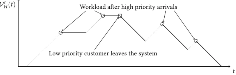
In theworkload processbased approach the first step of the solution is the stationary analysis of the workload of the system. The workload (or backlog) of the system increases at arrival instants by the amount of work brought into the system, and decreases at a slope of one between arrivals expressing that the server is processing the backlog (see Figure27). The sojourn time and waiting time related performance measures are given by the workload at arrival instants. The queue length properties, however, are a bit more challenging to derive by this method.
The age process based approach derives all performance measures from the age process, which represents the age of the oldest customer (the total time spent) in the system (Figure 25). It increases by a slope of one, and decreases at customer departures, when the next (younger) customer becomes the oldest one. The sojourn time of a customer is its age right
6 introduction
before the departure, and the queue length is the number of arrivals during the age of the oldest customer.
The queue length process based analysis of queues like the MAP/PH/1, MAP/G/1, G/MAP/1, etc. queues leads to Markov chains with a regular block structure, that can be solved efficiently by matrix-analytic methods since the late 1980s. The sojourn time properties of these queues are much easier to characterize based on the workload or the age process, that, as opposed to the queue length process, are continuous state processes, for which the solution method- ology appeared only later. Some important results were published in [75] and [78], but the numerically efficient (matrix-analytic) solution became possible only by the combination of [71] and [28], since year 2005. Furthermore, it has been recognized that the workload and age process based approaches are the only reasonable ways to analyze multi-type queues like the MMAP[K]/PH[K]/1 and the MAP/G/1-Priority queues [41,78].
Consequently, the matrix-analytic solution of the workload and age processes, and its ap- plication to the analysis of multi-class queues is a recent, elegant, and very effective analysis technology in modern queueing theory.
In this dissertation all three solution approaches are applied for different purposes.
1.2.3 Queueing networks
Open queueing networks are popular modeling tools for the performance analysis of com- puter and telecommunication systems. Exact solution methods are available only for net- works with Poisson traffic input, specific service time distributions and service disciplines.
These restrictive assumptions make the exact solutions unlikely to use in the practice. The main reason is that in real systems the Poisson process is usually not a good model for the traffic behavior. Instead, the real traffic can be bursty and correlated, and the service times in the service stations can be correlated as well. Since these features have an impact on the performance measures, they have to be taken into consideration.
The attempts to analyze queueing networks with non-Poisson traffic and non-exponential service time distributions dates back to the second half of the last century. The first attempts were to consider the second moments of the inter-arrival and the service time distributions in the computations. A widely applied approximation of this kind was integrated into the QNA tool [87,88]. The intrinsic assumption in these approximations is that the consecutive inter- arrival times and the consecutive service times are independent. The evolution of packet switched communication networks during the eighties and nineties resulted in traffic with significant correlation which lead to the development of new modeling paradigms.
Several modeling approaches were developed to describe the properties of packet traffic better [73]. One of the lines of research is based on Markovian models with the aim of ex- tending the Poisson arrival process in order to capture more statistical properties of the traffic behavior. A long series of efforts resulted in the application ofMAPs. The main advantage of usingMAPsfor traffic description of queues is that they are closed for the basic traffic oper- ations like superposition and splitting, and that the queueing models driven byMAPscan be solved in a numerically efficient way by matrix-analytic methods. UsingMAPsfor the traffic description gave a new impulse to the research on queueing network analysis [74,42].
In this dissertation we present a new method along this line of research which is based on a recent result about the joint moment based representation ofMAPs.
1.3 the structure of the dissertation 7
1.3 the structure of the dissertation
The topic of PartIof the dissertation is workload modeling.
Chapter2introduces thePHdistribution and its main properties. PHdistributions will be used to represent the service times in the queueing models defined throughout the disserta- tion. It is demonstrated that aPHdistribution can have many representations. Various tools and theorems are provided to perform representation transformations. After these preliminar- ies, the canonical representations are introduced, which, apart of their theoretical importance, are shown to be beneficial forPHfitting as well. The chapter ends with a moment match- ing method based on a special, so-called generalized hyper-Erlang representation, that will be used many times in the subsequent chapters.
The MAPs, and their multi-class extensions, the marked Markovian arrival processes (MMAPs) are discussed in details in Chapter 3. After introducing the representation trans- formations and the significance of Markovian representations, the main results are presented, namely the lag-1joint moment based representation ofMAPs, and the corresponding moment matching method. The results in this chapter can be applied to createMAPs based on em- pirical measurement data. Furthermore, the joint moments play a principal role in the novel queueing network analysis approach introduced in the last chapter.
ThePHdistributions andMMAPsobtained by the presented procedures can be applied to represent packet service times and packet inter-arrival times for both analytical and simula- tion based performance evaluation of telecommunication systems.
The performance analysis of various queueing models are covered in PartIIof the disserta- tion.
Chapter4lays down the theoretical background by providing an overview on discrete and continuous state-space skip-free processes.
Chapter5is still an introductory chapter, that demonstrates how to use the queue length based, the workload process based and the age process based analysis techniques to obtain the performance measures of the well known MAP/MAP/1 queue. At the end of the chapter, the lag-1joint moments of the departure process are also derived that will be essential for the queueing network analysis.
The multi-type first-come-first-served (FCFS) MMAP[K]/PH[K]/1 queue is considered in Chapter6. What makes this system interesting is that it can not be solved by the classical queue length based approach. All performance measures, including the ones related to the departure process, are obtained from the age process.
In Chapter 7 an other multi-type system, with preemptive and non-preemptive priority queue is investigated. This system has been analyzed several times in the past, and the solu- tion is proven to be challenging. With some transformations of the workload process of the system, however, it becomes possible to derive all performance measures efficiently.
The results of all the above mentioned chapters are integrated in Part III, where a novel queueing network solution approach is described. In the proposed method the traffic of the internal links of the network are characterized byMAPs, that are created from the lag-1joint moments of the departure processes of the associated queues. The presented numerical exam- ples demonstrate that this approach has several advantages: theMAPsof the internal traffic are compact, there are no scalability problems, and the performance measures approximate the exact results with a reasonable accuracy.
Part I
W O R K L O A D M O D E L I N G
2
P H A S E -T Y P E D I S T R I B U T I O N S
Phase-type distributions are non-negative distributions with a Markovian structure [65,57].
Due to their computational advantages and easy integration in complex stochastic models, they are widely used for modeling the workload in telecommunication systems.
2.1 introduction to phase-type distributions 2.1.1 Matrix-exponential distributions
Before providing the definition of PH distributions we first define the more general matrix-exponential (ME) distributions. Historically,PHdistributions were introduced before MEdistributions, but to show their (non-trivial) relation it is better to discuss them in the re- verse order.
Definition 1. A row vector σ = {σi, i = 1, . . . ,N}, σ1 = 1 and square matrix S = {qij, i,j = 1, . . . ,N}define aMEdistribution if the probability density function (pdf) given by
f(x) =σeSx(−S)1 (1)
is non-negative forx ≥0.
The vector-matrix pair(σ,S)is called therepresentationof theMEdistribution, andNis the size of the representation. From (1) it follows that the cumulative distribution function (cdf) denoted byF(x), the Laplace-Stieltjes transform (LST) of thecdf f∗(s)and thekth moment of a ME(σ,S) distributed random variableF are
F(x) =P(F <x) =1−σeSx1, (2)
f∗(s) =E(e−sF) =σ(sI−S)−1(−S)1, (3) mk =E(Fk) =
Z ∞
0
xkf(x)dx= k!σ(−S)−k1, (4) where1is a column vector of ones andIis the identity matrix of appropriate size.
Definition 2. A(σ,S)representation is called aMarkovian representationif
• the entries of vectorσare valid probabilities (0≤σi ≤1,i=1, . . . ,N),
• matrixSis a valid generator of a transient continuous time Markov chain (CTMC), thus, qii<0andqij ≥0,∀i6= j,
• and for the row sum we have that∑Nj=1qij ≤ 0, i = 1, . . . ,N,with at least one state where the row sum is strictly negative.
12 phase-type distributions
Otherwise the representation is callednon-Markovian.
In the example below,(σ,S)is a Markovian, while(γ,G)is a non-Markovian representa- tion of aMEdistribution:
σ=h0.5 0.4 0.1 i
, γ= h0.3 −0.5 1.2 i
,
S=
−8 1 0
2 −6 4
0 2 −4
, G=
−7 2 1
5 −10 10
3 −2 −1
. (5)
The pdf f(x) can be expressed in a spectral form, too. Suppose the number of distinct eigenvalues of Sis nd. Let us denote the eigenvalues by −λi, and their multiplicity byri (∑ni=d1ri =K≤ N). From (1) we have
f(x) =
nd i
∑
=1ri
j
∑
=1bij(λix)j−1
(j−1)!λie−λix. (6)
Note that if λi ∈ C\Rthen ∃j 6= i : λj = λ¯i (λ¯i denotes the complex conjugate of λi).
To define a valid distribution the integral of the density function must exist, implying that the real part of all eigenvalues must be strictly negative, hence rehλii > 0,i = 1, . . . ,nd must hold. Furthermore, as a consequence of the Perron-Frobenius theorem the dominant eigenvalue (i.e., the eigenvalue with the largest real part) must be real.
WhenK = N, the(σ,S)representation is calledminimal. IfK < Nthen matrixShas at least one eigenvalue that does not play a role in thepdf, because the corresponding coefficient is zero.
2.1.2 Representation transformations
It is easy to see that the representation of aME distribution given by (σ,S)is not unique [26,66]. For instance, applying a permutation on the elements ofσandSleads to a different representation while the distribution remains obviously the same. However, there are many more possibilities to create different representations of the sameMEdistribution. Withany non-singular square matrixBsatisfyingB1=1thecdfgiven by (1) can be transformed as
F(x) =1−σeSx1=1−σBeB−1SBxB−11
=1−γeGx1, (7)
withγ = σBandG= B−1SB. Hence, representations(σ,S)and(γ,G)are different, but define the exactly samecdf, thus the exactly same ME distribution. For example, the two representations(σ,S)and(γ,G), as defined by (5), correspond to the same distribution, and the transformation matrix relating them is
B=
0.5 −1 1.5
0 0 1
0.5 0 0.5
. (8)
The definitions, results and properties regarding the representation transformation are elab- orated in the following theorems.
2.1 introduction to phase-type distributions 13 Theorem 1. [81] Let (σ,S) of sizeNand (γ,G) of sizeNrepresent twoMEdistributions withcdf FF(x)andFG(x), respectively. The two distributions are identical if there exists a non-singular matrixBof sizeN×N, such thatγ= σB,G=B−1SBandB1=1.
Proof. See (7) for the derivation.
Theorem1uses the square matrixBto transform between representations of the same size.
This operation is called asimilarity transformationin the sequel.
Definition 3. The similarity transformof(σ,S)with matrix Bis(σB,B−1SB)ifBis non- singular andB1=1.
The main properties of a similarity transformation are as follows (cf. [11])
• (σ,S)and(σB,B−1SB)have the same size,
• the eigenvalues ofSandB−1SBare identical,
• if(σ,S)is Markovian then(σB,B−1SB)can be both Markovian and non-Markovian.
Representations with different sizes can be transformed into each other in a similar manner, using a non-square transformation matrix. This is stated by the following two theorems, which are symmetric to each other.
Theorem 2. [66,21] Let (σ,S) of sizeNand (γ,G) of sizeM(M> N) be twoMEdistributions with cdfFF(x) and FG(x), respectively. If there exists a matrixV of size M×N, such that σ=γV,V S=GV,V1=1then the distributions given by (σ,S) and (γ,G) are identical.
Proof. Ifσ=γV,V S= GV,V1=1then FF(x) =1−σeSx1=1−σ
∑
∞ i=0Sixi
i!1=1−γV
∑
∞ i=0Sixi i!1
=1−γ
∑
∞ i=0Gixi
i!V1=1−γ
∑
∞ i=0Gixi
i!1=1−γeGx1= FG(x).
(9)
Theorem 3. [21] Let (σ,S) of sizeNand (γ,G) of sizeM(M > N) be twoMEdistributions with cdfFF(x)and FG(x), respectively. If there exists a matrixW of size N×M, such that σW =γ,SW =W G,W1= 1then the distributions given by (σ,S) and (γ,G) are identical.
Proof. IfσW =γ,SW =W G,W1=1then FF(x) =1−σeSx1=1−σ
∑
∞ i=0Sixi
i!1=1−σ
∑
∞ i=0Sixi i!W1
=1−σW
∑
∞ i=0Gixi
i!1=1−γ
∑
∞ i=0Gixi
i!1=1−γeGx1= FG(x).
(10)
For equivalent representations with different sizes we have the following properties.
• The eigenvalues ofSare all eigenvalues ofGwith at least the same multiplicity.
• If(σ,S)is Markovian then(γ,G)can be either Markovian or non-Markovian.
14 phase-type distributions
σ2=0.4
σ1=0.5
σ3=0.1 1 2
4 2
7
2
Figure 1.: The transient Markov chain belonging to (5)
σ1 =1
λ λ λ λ
Figure 2.: An Erlang distribution
2.1.3 Phase-type distributions
PHdistributions of size N are the subclass of MEdistributions of the same size having a Markovian representation.
If(σ,S)is a Markovian representation of a MEdistributed random variable F, then the correspondingPHdistribution has a probabilistic interpretation: F is the time to absorption of a transient Markov chain with sub-generatorSand initial state probability vectorσfor the non-absorbing states. The transient Markov chain and the initial state probabilities belonging to(σ,S)defined in (5) are depicted in Figure1.
There exist order N non-Markovian (σ,S) representations that define a valid (non- negative) density function but can not be transformed to an order N Markovian represen- tation. These distributions do not belong to thePHclass, while they are stillMEdistributions.
Consequently, the set ofMEdistributions is a superset of the one ofPHdistributions, thus we havePH(N)⊂ ME(N).
The significance ofPHdistributions in Markovian performance modeling is a consequence of two properties. First, it is proven in [67] thatPHdistributions form a dense subset of the set of all positive-valued distributions, which means that any distribution having a positive density in(0,∞)can be approximated arbitrarily well by aPHdistribution. The second ben- efit of usingPHdistributions is their closeness on many operations: the sum, the minimum and the maximum of independentPHdistributed random variables arePHdistributed as well.
2.1.4 Important representations
There are some particular, frequently used representations ofPHdistributions.
The most well-knownPHsub-classes are the Erlang (Figure2), the hyper-exponential and the hyper-Erlang (Figure3) distributions. These distributions have especially simplepdfand moment formula, enabling efficient simulation, moment matching, fitting, and analytical stud- ies.
There are two further representations playing an essential role in the theory ofPHdistri- butions: the acyclic and the monocyclic representations.
2.1 introduction to phase-type distributions 15
σ1
σ2
σ3
λ1
λ2
λ3
σ1
σ2
σ3
λ1 λ1
λ1
λ2
λ3 λ3
Figure 3.: Hyper-exponential and hyper-Erlang distributions
σ1 σ2 σ3 σ4
λ1 λ2 λ3 λ4
Figure 4.: One of the canonical forms of acyclic PH distributions
a c y c l i c p h d i s t r i b u t i o n s have either upper or lower triangular generators, thus their state transition graph does not have any loops. Their distinguishing feature is that they haveminimal,unique(so-calledcanonical) representations. In [26] three such canonical forms have been defined, the first one (for four states) is depicted in Figure4. This structure consists of a row of exponential stages with possibly different, but increasing transition rates, and an arbitrary initial distribution. In the following example(σ,S)is an acyclic representation and (γ,G)is its canonical form:
σ=h0.1 0.2 0.7 i
, γ=h0.34 0.3 0.36 i
,
S=
−5 2 1
0 −4 3
0 0 −2
, G=
−2 2 0
0 −4 4
0 0 −5
. (11)
m o n o c y c l i c r e p r e s e n tat i o n s have been defined in [64]. They consists of feedback Erlang blocks (FEBs) arranged in a row. The ithfeedback Erlang block FEBiis char- acterized by a rate parameterνi, a size parameterkiand a feedback probabilityzi(see Figure 5, wherek1=1,k2 =4,k3=1).
Monocyclic representations have a unique feature phrased by the following theorem.
σ1 σ2 σ3 σ4 σ5 σ6
ν1 ν2 ν2 ν2 (1−z)ν2 zν2
ν3
FEB-1 FEB-2 FEB-3
Figure 5.: Monocyclic representation of a PH distribution
16 phase-type distributions
Theorem 4. [64] EveryMEdistribution has a finite-dimensional Markovian monocyclic repre- sentation, if the density function f(x) satisfies f(x)>0, x∈(0,∞).
[64] provides a constructive algorithm to obtain the appropriate Markovian monocyclic representation. The transformation of a non-Markovian representation(σ,S)to a possibly larger Markovian (monocyclic) representation(γ,G)consists of the following steps.
1. In the first step matrixGis constructed. EachFEBimplements one real eigenvalue or a conjugate complex eigenvalue pair ofS. Let us denote thejth eigenvalue ofSby−λj, or, if it is a complex conjugate eigenvalue pair, by−λj =aj+bjiand−λ¯j = aj−bji.
• Ifλj is real, the parameters of thejthFEBareνj =λj,kj =1,zj =0.
• Ifλj is complex, the parameters of the correspondingFEBare determined as kj =the smallest integer for whichaj/bj >tan(π/kj), (12) νj = 1
2
2aj−bjtanπ
kj +bjcotπ kj
, (13)
zj =
1−
aj−bjtanπ kj
kj
. (14)
With these parameters matrixGis Markovian by construction and contains all eigen- values ofSwith the proper multiplicities. However, the size of matrixGcan be larger than the size of matrix S, meaning that new eigenvalues are introduced. These extra eigenvalues can not play a role in thepdf, thus vectorγmust ensure that their coeffi- cients in the spectral form of thepdfare zeros.
2. The second step of the procedure is calculating the initial vectorγ. To this end, we need to obtain the transformation matrixW that transforms matrixSto matrixG.
According to Theorem3matrix W is the solution ofSW = W G,W1 = 1, which is a linear system of equations with regards to the entries ofW. With the presented construction of G, this linear system always has a unique solution. If the size ofSis N, and the size ofGisM, equationSW = W GhasN×M unknowns and defines N×Mequations. However, onlyN×M−Nequations will be independent, sinceN eigenvalues ofSandGare the same. By addingW1=1we getN×Mindependent equations and obtain a unique solution.
The initial vector is then given byγ=σW, which may contain negative entries, hence may not be a valid Markovian probability vector.
3. The third, last step is necessary only if vectorγis not a proper probability vector. In this case, an Erlang tail (a number of extra phases with the same transition rates) needs to be appended to the row ofFEBs. This Erlang tail is added to matrixG, the corresponding transformation matrixW is re-calculated, and we get a new initial vector. It is proven in [64] that an appropriate Erlang tail always makes the representation Markovian, if (σ,S)defines aMEdistribution with positive density. Unfortunately there is no explicit way to obtain the size and the rate parameters of the Erlang tail to be added. One can apply a simple heuristic algorithm that increases the size of the Erlang tail successively and applies the secant method to find the rate parameter that makesγa valid probability vector.
2.2 canonical forms 17
0.013545 0.0072743 0.010133 0.016458 0.075044 0.87755
1 2.8845 2.8845 2.883 3.3047
0.00148
3.3047
FEB-1 FEB-2 Erlang tail
Figure 6.: Monocyclic representation of example (15) As demonstration, the non-Markovian representation
σ=h0.1 0.2 0.7 i
, S=
−1 0 0
0 −3 0.2
0 −0.2 −3
, (15)
is transformed to a monocyclic representation with the procedure outlined above. The result- ing initial vector and transient generator are
γ=h0.013545 0.0072743 0.010133 0.016458 0.075044 0.87755 i
,
G=
−1 1 0 0 0 0
0 −2.8845 2.8845 0 0 0
0 0 −2.8845 2.8845 0 0
0 0.0014803 0 −2.8845 2.883 0
0 0 0 0 −3.3047 3.3047
0 0 0 0 0 −3.3047
,
(16)
and the corresponding state transition graph is depicted in Figure 6. The original (σ,S) representation has a real eigenvalue (λ1 = −1), and a complex conjugate eigenvalue pair (λ2,3 = −3±0.2i). The first, degenerateFEB(lacking a real feedback) realizesλ1. The sec- ondFEBrealizesλ2andλ3, but also introduces an extra eigenvalue. The initial vector ensures that the coefficient of this eigenvalue is zero in the spectral form of thepdf(see (6)). After the secondFEBan Erlang tail follows, with the eigenvalues introduced there having zero co- efficients as well. Without the Erlang tail (or with a shorter one) the initial vector remains non-Markovian, containing negative elements.
Theorem4has a striking consequence: every MEcan be converted to a PHdistribution with more states, blurring the difference between the two distribution classes.
2.2 canonical forms
As seen in the previous sections, the(σ,S)representation ofPHdistributions is known to be non-unique and can be non-minimal, thus there can be many(γ,G)representations defining the same distribution. Furthermore, the number of parameters (non-determined elements) of this representation is N2+N−1when the size of vector σ and square matrix S is N (sinceShasN2elements andσhasN−1), while the spectral form of thepdfof orderNPH distributions (6) has only at most2N−1parameters.
To overcome these drawbacks unique, minimal, hence canonical representations are re- quired. Canonical forms (among other benefits) make thePHfitting procedures more efficient,
18 phase-type distributions
p 1−p
λ1 λ2
Figure 7.: Canonical representation of PH(2) distributions
since the underlying optimization procedure does not have to go back and forth between very different representations of almost the same distribution.
As mentioned earlier, canonical representations are available for a long time for acyclicPH distributions ([26]). For general (non-acyclic)PHs, however, finding canonical forms is more challenging.
2.2.1 Canonical representation of PH(2) distributions
According to [25], any ME(2) distribution can be transformed to an acyclic form, for which a canonical form exists due to [26]. This way the same canonical form is applicable for all (not only acyclic and even for non-Markovian) PH(2) representations.
Theorem 5. The distribution sets ME(2), PH(2) and APH(2) are equivalent, i.e., ME(2) ≡ PH(2)≡ APH(2).
Proof. Based on the definition of these classes, we haveME(2)⊃PH(2)⊃ APH(2). Here, we only prove that any ME(2) distribution has an APH(2) representation.
From [25] we have that theLSTf∗(s)for a second-order representation(σ,S)has the form f∗(s) = 1+s/α
(1+s/λ1)·(1+s/λ2), (17)
where λ1 and λ2 denote the eigenvalues of −S. This LST corresponds to a valid density function if and only ifλ1,λ2andαare all real and
0<min(λ1,λ2)≤α≤ ∞ (18)
is satisfied.
Let us rewrite thisLSTas f∗(s) = 1−λ1/α
(1+s/λ1)·(1+s/λ2)+ λ1/α (1+s/λ2).
This structure reveals an analogy to a Laplace transform of a Bernoulli mixture of a hypo- exponential density and an exponential density, which leads us to the following matrix- exponential representation
γ=hp 1−p i
, G=
"
−λ1 λ1 0 −λ2
#
, (19)
withp=1−λ1
α . Figure7visualizes this acyclic PH(2) representation. It is easily verified that (3) with these settings forγandGyields (17). Due to condition (18), i.e., λ1 ≤ α, it follows 0≤ λ1 ≤1so that (19) is indeed a valid APH(2) representation.
2.2 canonical forms 19
p3 p2 p1
x3 x2 x1−x13
x13
Figure 8.: The structure of the considered PH(3) distribution
In the example below the non-Markovian(σ,S)representation is transformed to the canon- ical form(γ,G):
σ=h−1.4 2.4 i
, γ= h0.8 0.2i, S=
"
−22 24
−15 16
#
, G=
"
−4 4
0 −2
#
. (20)
The steps of the transformation were:
• creating matrixG, where−λ1and−λ2are the eigenvalues ofS,
• obtaining the transformation matrixBby solving the linear systemBG=SB,B1=1,
• obtaining the initial vector of the canonical form fromγ=σB.
2.2.2 Canonical representation of PH(3) distributions
Since the dominant eigenvalue must be real, thepdfof PH(2) distributions can not have com- plex eigenvalues. Order-3 PHdistributions, however, can have complex eigenvalues. This essential difference leads to a more complicated canonical form, which is more involved to derive.
In [40] it is proven that every PH(3) distribution given by aMarkovian representationcan be transformed to aunicyclicform (see Figure8), which is almost the same as a canonical acyclic structure, but has an extra feedback arc.
The theorem below summarizes the results of [40].
Theorem 6. [40] If(σ,S)is a Markovian representation of a PH(3) distribution then it can be similarity transformed to the Markovian unicyclic representation
γ=hγ1 γ2 γ3i, G=
−x1 0 x13 x2 −x2 0
0 x3 −x3
, (21)
wherex1≥ x2 ≥x3 >0, 0≤x13< x1,0≤γ1,γ2,γ3,γ1+γ2+γ3 =1.
The structure of the resulting unicyclicPHdistribution is depicted in Figure8.
Theorem6and the corresponding algorithm assume that the initial representation(σ,S)is Markovian; if this assumption is violated, hence the input is a non-Markovian representation, the algorithm returns invalid results with possibly complex entries. This assumption can be restrictive in many situations including moment matching (discussed later in Section 2.3), since the moment matching procedures typically return non-Markovian representations.
20 phase-type distributions
Hence, in the rest of this section we introduce an alternative algorithm that is able to per- form the canonical transformation ofanynon-Markovian(σ,S)representations as well.
Let λ1,λ2,λ3 denote the eigenvalues of −S which are ordered such that rehλ1i ≥ rehλ2i ≥rehλ3ianda0,a1,a2the coefficients of the characteristic polynomial of−S, i.e.,
a0 =λ1λ2λ3, a1=λ1λ2+λ1λ3+λ2λ3, a2 =λ1+λ2+λ3. (22) The next lemma provides the similarity transformation matrix B connecting (σ,S)and (γ,G), and relates its elements with the coefficients of the characteristic polynomial.
Lemma 1. The similarity transformation matrixB, composed by the column vectors[b1,b2,b3], to transform an arbitrary size3matrixSto a unicyclic representation is given by
b1 = 1
x13−x1 S1,
b2 = 1
(x13−x1)x2 (x1I+S)S1,
b3 = 1
(x13−x1)x2x3 (x2I+S)(x1I+S)S1,
(23)
and
x13 =x1− a0 x21−a2x1+a1, x2 = a2
−x1+ q
(a2−x1)2−4(x21−a2x1+a1)
2 ,
x3 = a2
−x1−q(a2−x1)2−4(x21−a2x1+a1)
2 .
(24)
The proof of the Lemma can be found in AppendixB.1.
The transformation matrixBand the transformed unicyclic representationGdepend on the choice ofx1. [40] showed the following properties of PH(3) distributions and this similarity transform.
P1) WhenSis a Markovian generator then
ϑu= a2 +2
q
a22−3a1
3 , (25)
ϑ0 = a2 +
q
a22−3a1
3 , (26)
ϑ` = (
λ1, ifλ1 ∈R,
ϑ0, ifλ1 ∈C (27)
are real and positive such thatϑ` ≤ϑu.
P2) Whenϑ` ≤ x1≤ ϑuthen the transformed generator matrix,G= B−1SBis Markovian such thatx1 ≥x2 ≥x3>0.
Indeed, property P2 holds also for any non-Markovian matrixSif its eigenvalues satisfy the requirements of PH(3) distributions: