Policies. University of Szeged, Doctoral School in Economics, Szeged, pp. 135–159.
Capital flight and external debt in Heavily Indebted Poor Countries in Sub-Saharan Africa: An
empirical investigation
Isaac Kwesi Ampah – Gábor Dávid Kiss – Balázs Kotosz
Over the past few decades, Sub-Saharan African countries, in their bid to achieve economic growth and development have resorted to external borrowings, propelling them to the status of Heavily Indebted Poor Countries (HIPC), when their debt reached unsustainable levels in the early 2000s. Unfortunately, the economies of these countries reported only steady growth with successive periods of high inflation and undesirable balance of payments deficits, leading scholars to ask whether external debt really can contribute to growth. At the same time, there is now considerable evidence that the build-up in debt was accompanied by increasing capital flight from the region. Employing Pooled Mean Group (PMG) estimation and datasets from 1990 to 2012, this paper investigated the apparent positive relationship between capital flight and external debt in Sub-Saharan Africa, taking Heavily Indebted Poor Countries in the region as a case study. The results revealed that external debt exerted a positive and statistically significant effect on capital flight both in short and long-run, suggesting that if foreign borrowing remains unchecked, it will continue to lead to massive capital outflow in Heavily Indebted Poor Countries in Sub-Saharan Africa.
Keywords: Sub-Saharan Africa; external debt; capital flight; cointegration; Pooled Mean Group, Heavily Indebted Poor Countries (HIPC)
1. Background of the study
External borrowing is a common phenomenon in many developing countries especially in their early stages of economic development as they are confronted with limited domestic resources for investment (Todaro–Smith 2006). So a developing nation with meager savings needs to borrow more to finance the optimal level of economic growth and development it desires for its people. Thus, external debt is often obtained incurred to supplement domestic resources to fund the current account deficits arising from external disturbances, and also to strengthen the external liquidity position of the country, which otherwise would not be possible with the domestic resources available. Safdari and Mehrizi (2011), posit that foreign borrowing is desirable and necessary to accelerate economic growth since the interest rates normally charged by the international financial institutions like the International Monetary Funds (IMF) and the World Bank are about half those charged by the domestic financial institutions.
The subject of external debt, especially that of Sub-Saharan Africa, has been at the forefront of international discussion for the past three decades. Adepoju
et al. (2007) noted that insufficient internal capital formation is often a characteristic of developing countries in Sub-Saharan Africa, mainly due to the vicious circle of low productivity, low income, and low savings, and as a result, they have usually adopted a development policy framework that is highly dependent on foreign borrowing from both official and unofficial sources. According to Ajayi and Khan (2000), this means that for many countries in the continent, the amount of external debt accumulated over recent decades amounts to what is seen as an unsustainable position. From a level of US$176.36 billion in 1990, total external debt stocks of SSA rose to US$235.94 billion in 1995. During the same period, external debt as a percentage of GDP increased from 58.21% to 71.95% respectively. For the years under study (1990–
2012), the highest external debt to GDP ratio of 78.23 percent was attained in 1994.
With the total external debt stock standing at US$213.44 billion in 2000, their value rose by US$55.63 billion by the end of 2010, reaching US$269.08 billion. External debt witnessed a rapid build-up for the three-year period (2010–2013), increasing by US$ 98.43 billion (from US$269.08 billion to US$367.51 billion), representing 77 percent greater increase on than the increment realized during the previous decade (2000–2010).
The massive growth in external debt in Sub-Saharan Africa, according to policymakers, is thwarting the continent’s prospects and efforts in achieving increased saving and investment, which consequently stymies economic growth and poverty reduction, principally known as the "debt overhang" effect. The debt overhang of the region has affected public investment in both physical and social infrastructure due to the massive outflow of resources in debt-service payments. Similarly, it has also inhibited private investment, since private investors are typically wary of policy distortions in environments marred by severe external imbalances and fluctuating exchange rates. By investing less in public health, social infrastructure, and human resource development, the implication is drawn that the external debt burden has compromised some of the essential conditions for sustainable economic growth and poverty reduction.
Furthermore, as the severity of external debt becomes more pronounced, there is considerable evidence that capital flight from the region is also increasing at a higher pace. Recent estimates suggest that capital flight has increased even more rapidly, and could amount to over twice the size of the external debt. Considering this emerging trend, a growing number of researchers have characterized the Sub-Saharan Africa region as “net creditor” to the world (Boyce–Ndikumana 2012). For instance, the latest estimates of capital flight show that Sub-Saharan African lost a total of $814.2 billion between the 1970-2010 periods. This stock of capital flight including compound interest earnings reached $1.06 trillion, which slightly exceeds the combined economic size of the countries as measured by their GDP ($1.05 trillion in 2010). The stock of capital flight also exceeds the $188.6 billion of external debt owed by these countries, making them as a group a ‘net creditor’ to the rest of the world. In
other words, these countries could go debt free if they could recuperate just 18 percent of the capital they have lost in unrecorded outflows. Again, this amount exceeds both the $659.5 billion in official development aid and $306.4 billion in Foreign Direct Investment for the same period (Boyce–Ndikumana 2011). Collier et al. (2001) also found evidence that compared to other developing regions, Sub-Saharan Africa has a greater share of private wealth being held abroad
It is against this background that this study has been conducted to empirically examine the long- and the short-run relationship between capital flight and external debt in HIPC countries in Sub-Saharan African, using time series datasets from 1990 to 2012. By estimating this relationship, the study hopes to shed some light on how to move forward by offering possible solutions for dealing with these issues. This study is organized into five parts. The first part, which is the introductory chapter, presents a background to the study providing a statement of the problem, the objectives of the study, as well as the scope and organization of the study. The second part presents a review of relevant literature, comprising both theoretical and empirical reviews. This section also looks at the trend of external debt and capital flight in HIPC countries in Sub-Saharan African. The third section presents the methodological framework and techniques employed in conducting the study. Section four examines and discusses the results, and major findings concerning the literature and the final part present the findings and policy implications of the study.
2. Literature Review
2.1. Theoretical and empirical literature review
The relationship between external borrowing and capital flight has been well documented in the literature, which recognizes that annual flows of foreign borrowing constitute the most consistent determinant of capital flight. A review of the literature suggests that the simultaneous occurrence of capital flight and foreign debt in a country is theoretically plausible. In the case of Argentina, Dornbusch and de Pablo (1987) noted that commercial banks in New York had lent the government the resources to finance capital flight which returned to the same bank as deposits. In a sample of 30 Sub-Saharan countries over the period 1970-96, Ndikumana and Boyce (2003) found that for every dollar of external debt acquired by a country in SSA in a given year, on average, roughly 80 cents left the country as capital flight. Their results also support the hypothesis by Collier et al. (2001) that a one-dollar increase in debt adds an estimated 3.2 cents to annual capital flight in subsequent years. This result leads to the question of why countries borrow so heavily while at the same time capital is fleeing abroad. From the literature, there are two main points of view:
- the indirect theory by Morgan Guaranty Trust Company (1986);
- Direct Linkages Theories by Boyce (1992).
2.1.1. Indirect theory
According to Morgan Guaranty Trust Company (1986) view, the simultaneous occurrence of external debt accumulation and the outflow of capital from developing countries is not a natural coincidence, but rather the track record of bad policies that have caused capital flight to arise are the very same policies responsible for increases in external debt accumulation. This view of external debt and capital flight linkage maintains that the relationship between the two may be attributed to poor economic management, policy mistakes, corruption, rent-seeking behavior, weak domestic institutions, and the like. For instance, the Morgan Guaranty Trust Company (1986) contends that indirect factors such as low economic growth regimes, overestimated exchange rates, and poor fiscal management by governments of developing countries are not only the cause of capital flight but also generate demand for foreign credit.
Another contention of the indirect theory by Morgan Guaranty Trust Company (1986) is that capital inflows (especially during surges of capital flows) lead to risky or unsound investment decisions and over-borrowing. For instance, when governance structures and mechanisms for administrative controls and prudential regulation are weak, fragile or absent, money borrowed from abroad can end up being pocketed by the domestic elite (and usually transferred into private accounts abroad). These fund are spent on conspicuous consumption or allocated to showcase unproductive development projects that do not generate foreign exchange or to finance external debt servicing. So capital flight and external borrowing are manifestations and responses to unfavorable domestic economic conditions.
2.1.2. Direct Theory
According to Ayayi (1997), the direct linkages theory contends that external borrowing directly causes capital flight by providing the resources necessary to affect flight. Cuddington (1987) and Henry (1986) showed that in Mexico and Uruguay, capital flight occurred contemporaneously with increased debt inflows, thus attesting to a strong liquidity effect in these countries. According to this theory, external resources acquired as loans can create conditions for capture as “loot” that individuals (often the elite) appropriate as their own. In fact, according to Beja (2006), the (captured) funds may not even enter the country at all. Instead, mere accounting entries are entered in the respective accounts of the financial institutions. Boyce (1992) further distinguishes four possible, equivalent links between external debt and capital flight.
The first is the debt-driven capital flight. According to Boyce (1992), in a debt- driven capital flight, residents of a country are motivated to transport their assets to foreign countries due to excessive external borrowing by the domestic government.
The outflow of capital is, therefore, in response to fear of the economic consequences
of heavy external indebtedness. So the desire to avoid such taxes in the future causes individuals within the country to transport their capital abroad.
The second is debt-fueled capital flight. According to Boyce (1992), in a debt- fueled capital flight, the external debt acquired provides both the reason and the resources needed for capital flight. Suma (2007) identifies two processes that debt- fueled capital flight occurs. First, the domestic government acquires the foreign capital, then sells the resources to the domestic residents who later transfer them abroad either by legal or illegal means. Secondly, the government can lend the borrowed funds to private borrowers through a national bank, and the borrowers, in turn, transfer a part or all of the capital abroad. In this case, external borrowing provides the necessary fuel for capital flight (Ajayi 1997).
Meanwhile, Flight-driven External Borrowing is a situation where after the capital flight, which dries up domestic resources, the gap between savings and investment rises, so the government borrows more resources from external sources to fill the resource gap created in the domestic economy. This situation occurs due to resource scarcity in the domestic economy, with both the public and private sectors seeking replacement of the lost resources by acquiring more loans from external creditors. The external creditors’ willingness to meet this demand can be attributed to different risks and returns facing residents and non-resident capital. “The systemic differences in the risk-adjusted financial returns to domestic and external capital could also arise from disparities in taxation, interest rate ceilings and risk-pooling capabilities” (Lessard–
Williamson 1987, p. 215).
Finally, Flight-fueled External Borrowing occurs when the domestic currency siphoned out of the country through capital flight re-enters in the form of foreign currency that finances external loans to the same residents who transferred the capital.
In other words, the domestic capital is converted to foreign exchange and deposited in foreign banks, and the depositor then takes a loan from the same bank in which the deposit may serve as collateral. This phenomenon is also known as round-tripping or back-to-back loans (Boyce 1992).
At the empirical level, Saxena and Shanker (2016) examined the dynamics of external debt and capital flight in the Indian economy; the authors using Two Staged Least Square (2SLS) method, investigate the relationship of the two during the period 1990-2012. The result of the study indicates a positive correlation between external debt and capital flight in India. Usai and Zuze (2016) provided a similar analysis for Zimbabwe using Vector Autoregression. The main objective of their study was to establish the direction of causality between capital flight and external debt for the period 1980-2010 in the essence of the revolving door hypothesis. Their study employed the Granger causality test to investigate this relationship. The pairwise Granger causality test revealed the existence of a unidirectional relationship running from external debt to capital flight. Their result indicates that for Zimbabwe, external debt has influenced capital flight and not the other way round.
Abdullahi et al. (2016), also examine the impact of external debt on the growth and development of capital formation in Nigeria. Time series data were used for a period from 1980 to 2013, employing Autoregressive Distributed Lag (ARDL) modeling. The result of stationarity tests showed that the variables are both I(0) and I(1) necessitating the use of ARDL. ARDL estimation also revealed the presence of a long run relationship amongst the variables. However, the study showed that the variables were related independently in the long-run. The result also indicated a negative and statistically significant association between external debt and capital formation with savings leading to a bidirectional causality relationship amongst the variables. The interest rate was also statistically significant even though it was weak.
The other variables were found to be of unidirectional causal effects.
Boyce and Ndikumana (2012) also examine the impacts of capital flight with linkages to external borrowing in Sub-Saharan Africa. The results of the study established that Sub-Saharan Africa is a net creditor to the rest of the world because the private external assets exported exceed its external public liabilities. This finding suggests the existence of debt-fueled capital flight. The results also show a debt overhang effect, as increases in the debt stock spur additional capital flight in later years and underscore the exploitation of natural resource-rich countries. The studies also emphasize the significant role of government institutions and structures in alleviating the dangers of capital flight, while political uncertainty is found to be a key determinant of capital flight. McCaslin (2013) also explored estimates of capital flight from Portugal, Italy, Greece and Spain (PIGS) during the Eurozone debt crisis and examined the determinants of capital flight from the distressed PIGS zone.
Demachi (2013) in his study, examine the impact of international resource price increases on capital flows from twenty-one (21) resource-rich developing countries (RRDCs) from 1990-2011. The results of his analysis suggested the need to focus more on capital outflow from RRDCs through transnational companies.
In a nutshell, the relationship between capital flight and external debt have been the focus of many types of research and policymakers. Under conventional expectations, the bidirectional relationship between capital flight and external debt, which is also known as the revolving door hypothesis, seems to be the more common research finding.
3. Methodology
3.1. Data sources and scope
The study uses secondary data mainly drawn from the World Bank (World Development Indicators, International Financial Statistics) and the African Bank Development Indicators 2016 online databases. HIPC countries in Sub-Saharan Africa comprise 30 countries, however, due to data unavailability on some relevant variables for some countries, annual data for 26 HIPC countries in Sub-Saharan Africa
countries were used in the study for empirical analysis. Data on capital flight or external debt for the remaining four (4) countries in the Sub-Region is unavailable. It is likely that their participation in external debt or capital flight activities in the region is insignificant, and hence the empirical results based on the 26 countries in the region is expected to reveal the real situation among HIPC countries in SSA. The study covers a period of 23 years (1990-2012) which captures the long-term impacts of the 1982 global debt crisis, the effect of the 2008 financial crisis and the current economic downturn, on external borrowing and capital flight. However, data unavailability for some of the years mentioned represented a constraint in choosing the period of 23 years for the empirical analysis.
3.2. Model Framework
The traditional panel models, such as fixed effects, random effects, and pooled OLS models have certainly had some challenges. For example, pooled OLS is considered to be a highly restrictive model since it imposes a common intercept and slope coefficients for all cross-sections, and thus disregards individual heterogeneity. The fixed effects model, on the other hand, assumes that the estimator has common slopes and variance but country-specific intercepts. Even though the cross-sectional and time effects can be observed through the introduction of dummy variables in the fixed effect model, especially in a two-way fixed effects model, nevertheless, this estimator also suffers severe problems due to the loss of degrees of freedom according to Baltagi (2008). Additionally, the parameter estimates produced by the fixed effects model are biased when some regressors are endogenous and associated with the error terms as demonstrated by Campos and Kinoshita (2008). The random effects model is comparatively less problematic as regards the degrees of freedom, basically because it has an inherent assumption of common intercepts. However, the random effects model considers the model to be time-invariant which means that the error at any period is not associated with the past, present, and future, known as strict homogeneity by Arellano (2003). The main issue is that, in real life, this assumption is very often invalid. Furthermore, as Loayza and Ranciere (2006) argue, static panel estimators do not take into account the panel dimension of the data by distinguishing between short- and long-run relationships. Furthermore, conventional panel data models assume homogeneity of the coefficients of the lagged dependent variable (Holly–Raissi 2009), and this can lead to a serious bias, when in fact the dynamics are heterogeneous across the cross-section components. Therefore, the standard panel methods have been criticized for neglecting the dynamic nature of the data, which happens to be the central theme in the empirical literature. Moreover, they only focus on the structural heterogeneity of the model with regard to random or fixed effects, but enforce strict homogeneity in the model’s slope coefficients across countries, even when there may be significant distinctions among them.
In recent times, a lot more of the empirical studies have focused on the dynamic panel estimation method. However, according to Samargandi et al. (2015) and Roodman (2006), in the dynamic panel estimation, when there are a large number of countries compared to the time period, then the GMM-system estimator proposed by Arellano and Bover (1995) and the GMM-difference estimator by Arellano and Bond (1991) both work well. These two estimators are typically used to analyze micro panel datasets (Eberhardt 2012). However, a wide range of recent literature has applied GMM techniques to macro panel data, including from the area of capital flight and external debt (e.g. Fiagbe (2015) and Domfeh (2015)). However, GMM captures only the short-run dynamics, and the long-run relationships between the variables tend to be overlooked because these models are frequently restricted to short time series.
Pesaran and Smith (1995), Pesaran (1997) and Pesaran et al. (1999) present the autoregressive distributed lag (ARDL) model in error correction framework as a comparatively new cointegration test. However, the emphasis is on the need to have consistent and efficient estimates of the parameters both in the long- and short-run relationship. According to Johansen (1995) and Philipps and Bruce (1990), the long- run relationships exist only in the framework of cointegration between variables with the same order of integration. Pesaran et al. (1999) however, show that panel ARDL can be used even with variables with different orders of integration, and irrespective of whether the variables under study are I(0) or I(1) or a mixture of the two. This is a significant advantage of the ARDL model, as it makes testing for unit roots unnecessary. Also, the short-run and long-run effects can be estimated concurrently from a data set with large cross-section and time dimensions. Finally, the ARDL model provides positive coefficients despite the presence of endogeneity as it includes the lags of both the dependent and independent variables included in the model (Pesaran et al. 1999). This study, therefore, estimates the dynamic relationship between external debt and capital flight using the ARDL method. Specifically, the study will use the recent Pooled Mean Group (PMG) estimator. According to Samargandi et al. (2015), the main characteristic of the Pooled Mean Group estimator is that it permits the short-run estimates, the speed of adjustment to the equilibrium values of long-run, the intercepts and the error variances to be heterogeneous across countries, while the long-run slope coefficients are restricted to be homogeneous across countries.
The dynamic panel model of the study is specified as:
𝐶𝐹𝑖𝑡 = 𝛿𝐶𝐹𝑖𝑡−1+ 𝛽𝑋𝑖𝑡+ 𝑢𝑖+ 𝜀𝑖𝑡 (1) Where 𝐶𝐹 represents external debt, 𝑋 is the matrix of all the explanatory variables, 𝑢 denotes unobserved country-specific time-invariant effect, 𝜀𝑖𝑡 accounts for the stochastic error term, 𝛿, 𝛽 are the parameters to be estimated, 𝑖 stand for a particular country, and 𝑡 is time. Along the lines of the theoretical and empirical relationship
between capital flight and external debt postulated in the literature review, equation 1 has been consolidated with variables and rewritten as
𝐶𝐹𝑖𝑡 = 𝛼1+ 𝛽1𝐶𝐹𝑖𝑡−1+ 𝛽2𝐸𝑋𝑇𝑖𝑡+ 𝛽3𝐺𝐷𝑃𝑖𝑡 + 𝛽4𝐼𝑁𝐹𝑖𝑡+ 𝛽5𝑃𝑂𝐿𝐼𝑇𝑌𝑖𝑡+ 𝛽6𝐹𝐷𝑖𝑡+
𝑢𝑖+ 𝜀𝑖𝑡 (2)
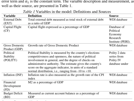
Here 𝐸𝑋𝑇 is total external debt, 𝐶𝐹 is capital flight, 𝐺𝐷𝑃 is the real gross domestic product growth rate, 𝐼𝑁𝐹 is inflation, 𝑃𝑂𝐿𝐼𝑇𝑌 represents political stability, 𝐵𝐷 represents budget deficit, and 𝐹𝐷 is financial development. Further, the coefficients, 𝛽1, 𝛽2 … 𝛽6, are the output elasticities of the factor inputs, while 𝜀𝑖𝑡 is the stochastic error term and 𝛼1 is the constant term. The variable description and measurement, as well as their source, are presented in Table 1.
3.3. Estimation technique
As a general method, cointegration techniques following Johansen (1991), Engle and Granger (1987), Phillips (1991), Phillips and Loretan (1991) and Phillips and Hansen (1990) are used to estimate long-run relationships between variables integrated of order one, so-called I(1) variables. The basic premise of cointegration literature is that long-run relationships exist only between the cointegrated variables. If the variables
Table 1 Variables in the model: Definitions and Sources
Variable Definition Source
External Debt (EXT)
Total external debt measured as total stock of external debt as a ratio of GDP
WDI database Capital Flight
(CF)
Capital flight expressed as a percentage of GDP Database of Political Economy Research Institute (PERI).
Gross Domestic Product (GDP)
Growth rate of Gross Domestic Product WDI database Political
Stability (POLITY)
Political Stability is measured by the country's elections competitiveness and openness, the nature of political involvement in general, and the degree of checks on administrative authority. The estimate gives the country's score on the aggregate indicator, in units of a standard normal distribution, i.e., ranging from -10 to +10.
Polity 2 data series from Polity IV database under
Inflation (INF) Inflation rate is also measured as the growth rate of the CPI index
WDI database Financial
Development (FD)
M2 as a percentage of GDP WDI database
Budget Deficit (BD)
Measured as current account balance as a percentage of GDP
WDI database Source: Constructed by the authors
are not integrated of order one, traditional regression estimations are no longer applicable. Pesaran et al. (1999) re-examined the use of the traditional ARDL approach for the analysis of long-run relations and showed that slight modifications to standard methods render consistent and efficient estimators of the parameters in a long-run relationship between both integrated and stationary variables.
One very prominent feature of the autoregressive distributed lag (ARDL) approach to long-run modeling, as presented by Pesaran et al. is that it is not necessary to pre-test the stationarity or confirm the degree of integration of the variables of interest. The reason is that the estimate of the ARDL is still valid whether or not the variables of interest are interested of I(0) or I(1) or mutually cointegrated. Another advantage of ARDL method is that estimation is possible when explanatory variables are endogenous. Furthermore, a dynamic error correction model (ECM) can be derived from ARDL that integrates the short-run dynamic with the long-run equilibrium without losing long-run information. The study estimates the ARDL using the Pooled Mean Group (PMG) estimator of Pesaran et al. (1999), and a panel consisting of the 26 Heavily Indebted Poor Countries in Sub-Saharan Africa and spanning the years 1990 to 2012. The use of the PMG offers some advantages. It allows the short-run coefficients, with the intercepts, the speed of adjustment to the long-run equilibrium values and error variances to be heterogeneous among countries, while the long-run slope coefficients are limited to be homogeneous across countries.
This is particularly important when there are reasons to suppose that the long-run equilibrium relationship between the variables is parallel across countries or, at least, a subset of them. Meanwhile, the short run adjustment is allowed to be country- specific, due to the widely different impact of capital flight on external debt. This framework is implemented by modeling equation (2) as:
Δ𝐶𝐹𝑖𝑡 = 𝛽0+ 𝛽1𝐶𝐹𝑖𝑡−1+ 𝛽2𝐸𝑋𝑇𝑖𝑡−1+ 𝛽3𝐺𝐷𝑃𝑖𝑡−1+ 𝛽4𝐼𝑁𝐹𝑖𝑡−1+
𝛽5𝑃𝑂𝐿𝐼𝑇𝑌𝑖𝑡−1+ 𝛽6𝐹𝐷𝑖𝑡−1+ 𝛽7𝐵𝐷𝑖𝑡−1+ ∑𝑝𝑗=1𝛼1𝑗Δ𝐶𝐹𝑖𝑡−j+ ∑𝑝𝑗=1𝛼2𝑗Δ𝐸𝑋𝑇𝑖𝑡−𝑗+
∑𝑝𝑗=1𝛼3𝑗Δ𝐺𝐷𝑃𝑖𝑡−𝑗+ ∑𝑝𝑗=1𝛼4𝑗Δ𝐼𝑁𝐹𝑖𝑡−𝑗+ ∑𝑝𝑗=1𝛼5𝑗𝑃𝑂𝐿𝐼𝑇𝑌𝑖𝑡−𝑗+
∑𝑝𝑗=1𝛼6𝑗𝐹𝐷𝑖𝑡−𝑗+ ∑𝑝𝑗=1𝛼7𝑗𝐵𝐷𝑖𝑡−𝑗+ 𝑢𝑖+ 𝜐𝑖𝑡 (3) Here Δ denotes the first difference operator, 𝑃 is the lag order selected by Akaike’s Information Criterion (AIC), 𝛽0 is the drift parameters while 𝜐𝑡 is the white noise error term which is ~𝑁 (0, 𝛿2). The parameters 𝛼𝑖 are the short-run parameters and 𝛽𝑖 are the long-run multipliers. All the variables are defined as previously described.
Given that cointegration has been established from the model, the next step is to estimate the long run and error correction estimates of the ARDL and their asymptotic standard errors. The long run is estimated by:
𝐶𝐹𝑖𝑡 = 𝜇0+ ∑𝑝𝑗=0𝛽1𝑗𝐶𝐹𝑖𝑡−𝑗+ ∑𝑝𝑗=0𝛽2𝑗𝐸𝑋𝑇𝑖𝑡−𝑗+ ∑𝑝𝑗=0𝛽3𝑗𝐺𝐷𝑃𝑖𝑡−𝑗+
∑𝑝𝑗=0𝛽4𝑗𝐼𝑁𝐹𝑖𝑡−𝑗+ ∑𝑝𝑗=0𝛽5𝑃𝑂𝐿𝐼𝑇𝑌𝑖𝑡−𝑗+ ∑𝑝𝑗=0𝛽6𝐹𝐷𝑖𝑡−𝑗+ ∑𝑝𝑗=0𝛽7𝐵𝐷𝑖𝑡−𝑗+ 𝑢𝑖+
𝜐𝑖𝑡 (4)
This is followed by the estimation of the short-run parameters of the variables with the error correction representation of the model. By applying the error correction version of ARDL, the speed of adjustment to equilibrium is determined. When there is a long-run relationship between the variables, then the unrestricted ARDL error correction representation is estimated as:
Δ𝐶𝐹𝑡 = 𝜙0+ ∑𝑝𝑗=0𝛿1𝑗Δ𝐶𝐹𝑖𝑡−𝑗+ ∑𝑝𝑗=0𝛿2𝑗Δ𝐸𝑋𝑇𝑖𝑡−𝑗∑𝑝𝑗=0𝛿3𝑗Δ𝐺𝐷𝑃𝑖𝑡−𝑗+
∑𝑝𝑗=0𝛿4Δ𝐼𝑁𝐹𝑖𝑡−𝑗+ ∑𝑝𝑗=0𝛿5𝑗𝑃𝑂𝐿𝐼𝑇𝑌𝑖𝑡−𝑗+ ∑𝑝𝑗=0𝛿6𝑗𝐹𝐷𝑖𝑡−𝑗+ ∑𝑝𝑗=0𝛿7𝑗𝐵𝐷𝑖𝑡−𝑗+
𝛾𝐸𝐶𝑇𝑖𝑡−𝑗+ Ω𝑖𝑡 (5)
Here 𝛾 is the speed of adjustment of the parameter to long-run equilibrium following a shock to the system and 𝐸𝑋𝑇𝑡−1 is the residuals obtained from equations (4). The coefficient of the lagged error correction term 𝛾 is expected to be negative and statistically significant to further confirm the existence of a cointegrating relationship among the variables in the model. The value of the coefficient, 𝜆, which signifies the speed of convergence to the equilibrium process, usually ranges from -1 to 0. -1 signifies perfect and instantaneous convergence while 0 means no convergence after a shock in the process.
4. Empirical Result
4.1. Pattern of Capital Flight and external debt from HIPC Countries in Sub- Saharan Africa
The pattern analyses focus only on the 26 HIPC countries covered by the study for the period 1990-2012. Both capital flight and external debt are measured in millions of constant US dollars. Estimates presented in Figure 1 show that over the 23-year study period from 1990-2012, capital flight from HIPC countries in Sub-Saharan Africa has shown both upward and downward trends. However, the trend is positive across all the years except 1999. This suggests that HIPC countries in Sub-Saharan Africa are experiencing net capital outflow on a yearly basis. This positive outflow of capital in the region is attributed to the abundant oil and other natural resources the region possesses, poor governance, weak institutions, and the poor macroeconomic environment that has plagued the region.
Though the massive and continuous outflow of capital through illicit channels over the period 1990-2012 is a major issue for discussion, there are significant disparities in the regional pattern of illicit flows. Figure 2 shows that capital flight from West and Central Africa is the dominant driver of illicit flows from the HIPC Countries in Sub-Saharan region. The main reason for the difference probably may be a large number of HIPC countries in these sub-regions.
Figure 3 also depicts average illicit capital outflow among the HIPC countries in SSA during the study period. This analysis and findings provide an insight into where the concentration of capital flight in the sub-region is positioned, and as such the need for the entire region to help draw up policies and procedures to help curtail the phenomenon where it is endemic. The analysis of Figure 3 shows that Congo, Mozambique, and Ghana contribute substantially to capital flight in the region with the average capital flight ranging from 1200 million USD.
Figure 1 Pattern of capital flight in HIPC countries in Sub-Saharan Africa
Source: own construction
Figure 2 Regional pattern of capital flight
Source: own construction
Figure 4 shows that over the 23-year study period from 1990-2012, external debt from HIPC countries in Sub-Saharan Africa also showed both upward and downward trends, as was the case for capital flight. However, the trend increases outweighed the falls. For instance, Figure 1 shows that external borrowing from HIPC countries in the region increased from 1990 and reached a peak in the year 1998 before beginning to fall. However, it regained its rising disposition from 2001 reaching its highest in 2004 and then declined sharply again in 2006 only to turn upward again in 2007. The decline in 1998 through 2000 and 2004 through 2006 is attributed to the fiscal discipline that most of the countries engaged in to qualify for the HIPC relief in 2000 and multilateral debt relief in 2006. Total real capital flight in the combined HIPC in Sub-Saharan African countries has been growing since 2007.
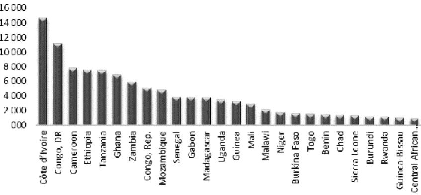
Figure 5 also shows the average capital flight estimates for HIPC countries in Sub- Saharan Africa for 1990-2012. Côte d’Ivoire has the largest amount of external borrowing among the HIPC countries in SSA. Burundi and the Central African Republic also have the lowest external debt among the HIPC countries in SSA.
Figure 3 Average capital flight for Sub-Saharan African countries
Source: own construction
Table 2 provides a summary of statistics relating to the twenty-six (26) HIPC countries in SSA for the period 1990–2012. The table indicates the summary descriptive statistics of central tendency and measure of variability. The mean values indicate the average value of the variables used in the overall model. The standard deviation also captures the distribution of data around the mean value. It also shows the closeness of data to the average value over the period under consideration. Also, the range indicates the spread of the data, and this is also measured by the maximum and minimum values in each different model. The range is an indicator of the level of variations in the variables. The larger the range values, the higher the degree of variations in a variable and vice versa. N, n, and T in the table represent the total observations, a total number of countries sampled and the total number of years for the study respectively. The mean of external debt of the sample is 82.6574 and ranges in value between 10.70016 and 304.851.
Figure 4 External debt for HIPC in SSA
Source: own construction
Figure 5 Average external debt for HIPC countries
Source: own construction
Over the period 1990–2012, the average external borrowing for the twenty-six HIPC countries in SSA under study averaged 87.02381 million constant US dollars, ranging from a maximum score of 10.70016 and 304.851 showing a high level of variation. The range of the capital flight (the main value of interest) indicates that between countries, observations (cross-sectional dimension) in the region attain scores as low as -0.1197744 and as high as 0.7770688 within the period under consideration, whereas, within countries, observation shows a wider variation (𝑙𝑜𝑤 =
−0.607496 and ℎ𝑖𝑔ℎ = 1.446824). The GDP index averaged 1.794359. Empirical studies on external debt in SSA is determined by the value of the political and functionality of the institution perception index. From Table 2 above, the maximum value of this variable observed is 9 with a minimum of -9. The total number of observation as indicated in the table is 460 with 23 years and 26 countries.
4.2. Panel unit root test
Though the Pooled Mean Group Estimation renders (panel) unit-root tests of the variables under study needless as long as they are I(0) and I(1), the study performed these tests nevertheless to ensure that no variable exceeded the I(1) order of integration, which would result in inconsistent estimations (Asteriou and Monastiriotis 2004). To do this, we applied three commonly used panel unit root tests.
The first is by Levin et al. (LLC) (1992), the second Im et al. (IPS) (1997), and finally Table 2 Descriptive statistics of the Data
Variable Mean Std. Dev. Min Max Observations
EXT Overall 82.6574 55.81469 10.70016 304.851 N = 460
Between 28.52664 39.04989 150.0186 n = 26
Within 48.37887 -44.70617 241.8563 T = 23
CF Overall 0.0980781 0.2646581 -0.546687 1.953331 N = 594 Between 0.1708889 -0.119774 0.777068 n = 26 Within 0.2043844 -0.607496 1.446824 T = 23 GDP Overall 6.214113 14.34703 -50.24807 105.2675 N = 598
Between 13.10628 -0.023571 69.88397 n = 26
Within 6.848762 -49.46443 41.59763 T = 23
INF Overall 61.24963 33.43816 4.13E-10 163.56 N = 598
Between 17.51328 19.82287 82.31043 n = 26
Within 28.70715 -0.579933 172.5453 T = 23
Polity Overall 0.4397993 4.845923 -9 9 N = 598
Between 3.411009 -4.73913 6.043478 n = 26
Within 3.503819 -12.73411 9.135452 T = 23
FD Overall 11.06982 6.751876 0.1982856 36.49501 N = 596
Between 5.392417 2.453031 21.7209 n = 26
Within 4.184846 0.2103994 28.89799 T= 23
Source: Authors’ own construction
the Fisher-Type Chi-square. These tests are founded on the assumption that all series are non-stationary under the null hypothesis but accounts for heterogeneity in the autoregressive coefficient, which is assumed to change freely among the states under study. The LLC test is appropriate because it can cover the most general specification for all the pooled variables with the inclusion of a constant, a trend and lags (Mathiyazhagan 2005). The advantage of the Fisher-Type unit root test is that it can be applied in almost every set of data (Durnel 2012). According to the test of Im et al.
(1997) that performed the Monte-Carlo simulations to equate the test that they suggested (IPS), and the Levin-Lin test, with the hypothesis of no cross-sectional correlation in panels, they showed that the IPS test is more powerful than the LL test.
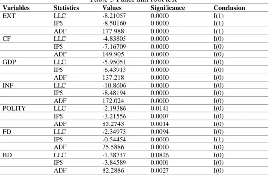
Table 3 presents the result of the unit root test.
The test results indicate that all the variables in the study are stationary at level except external debt and capital flight which is also significant at first difference. Due to the existence of mixed levels of integration among series, we proceeded to apply the Pooled Mean Group estimator rather than traditional static or panel cointegration test (Asteriou and Monastiriotis 2004). The Pooled Mean Estimator is characterized by multiplicities of advantages, of which it emphasizes and allows for the possibilities of estimating different variables with a different order of stationarity, as is the case in the study indicated in Table 3. We also noticed that our data suffers from either I(0) and I(1). On top of that these estimators allow us to estimate both short-run and long- run relationship along with the error correction coefficient.
4.3. Panel Cointegration Test
To determine whether a meaningful long-run relationship exists between the variables in our model, the study adopts the commonly applied Pedroni (2004) test, which accounts for heterogeneity by using specific parameters. This test offers eleven (11) panel statistics for which cointegration analysis can be made. The results of the test are given in Table 4. The results indicate a similar trend for both models with intercept only and the model with intercept and trend specifications. For the first model with intercept only, the null hypothesis of no cointegration is rejected at 1% level of significance for six out of the eleven test statistics. This means that six of the tests reject the null hypothesis of no cointegration indicating that cointegration exists.
Again, the second model also showed the same result for the cointegration analysis.
Given that six of the eleven test statistics concluded that there was cointegration between the variables under study, the study concluded that cointegration was present in the data and proceeded to the estimation using the mean group and pooled mean group estimator.
Table 3 Panel unit root test
Variables Statistics Values Significance Conclusion
EXT LLC -8.21057 0.0000 I(1)
IPS -8.50160 0.0000 I(1)
ADF 177.988 0.0000 I(1)
CF LLC -4.83805 0.0000 I(0)
IPS -7.16709 0.0000 I(0)
ADF 149.905 0.0000 I(0)
GDP LLC -5.95051 0.0000 I(0)
IPS -6.43913 0.0000 I(0)
ADF 137.218 0.0000 I(0)
INF LLC -10.8606 0.0000 I(0)
IPS -8.48194 0.0000 I(0)
ADF 172.024 0.0000 I(0)
POLITY LLC -2.19386 0.0141 I(0)
IPS -3.21556 0.0007 I(0)
ADF 85.2743 0.0014 I(0)
FD LLC -2.34973 0.0094 I(0)
IPS -0.54454 0.0000 I(1)
ADF 75.5886 0.0000 I(0)
BD LLC -1.38747 0.0826 I(0)
IPS -3.84589 0.0001 I(0)
ADF 82.2886 0.0027 I(0)
Note: LLC, IPS, and ADF are Levin et al. (2002); Pesaran Shin and Smith (1997) and Fisher Type ADF, respectively.
Source: own construction
Table 4 Panel Models
Panel Model A: Intercept Only Within Dimension
Statistic Probability Weighted Statistics Probability
Panel v-Statistic -1.329927 0.9080 3.415912 0.928
Panel rho-Statistic 3.352467 0.9942 2.141952 0.9816 Panel PP-Statistic -4.570207 0.0000 -8.691525 0.0000 Panel ADF-Statistic -7.353888 0.0000 -8.133307 0.0000 Between Dimension
Group rho-Statistic 4.643302 0.932
Group PP-Statistic -9.901646 0.0000
Group ADF-Statistic 8.222222 0.0000
Panel Model B: Intercept and Trend Within Dimension
Statistic Probability Weighted Statistics Probability
Panel v-Statistic -3.587684 0.9997 -5.46802 1.0000
Panel rho-Statistic 4.724599 0.9996 3.374462 0.99960 Panel PP-Statistic -5.286987 0.0000 -10.92029 0.0000 Panel ADF-Statistic 5.474111 0.0000 -7.56946 0.0000 Between Dimension
Group rho-Statistic 5.721004 1.0000
Group PP-Statistic -17.45533 0.0000
Group ADF-Statistic -8.299459 0.0000
Source: Computed by the authors using Eviews 9
4.4. Long-run and short-run results using the Pooled Mean Group Estimator (PMG) Given that cointegration had been established from the model, the study proceeded to estimate the long-run relationship and the short-run dynamics between the variables.
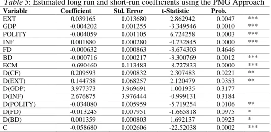
The result of the long-run and short-run relationship between capital flight and the independent variables are presented in Table 5 below. As revealed in Table 5, the results indicate theoretically correct and prior expected signs for almost all the explanatory variables. External debt expressed as a ratio of GDP, Real GDP growth, political stability, inflation and budget deficit all have the expected sign and exert a statistically significant effect on capital flight in the long-run. Financial development, however, is statistically insignificant; it has the expected sign. The constant is also negative and statistically significant too. The positive and statistically significant coefficient of the capital flight means that increases in capital flight have the potential to stimulate external debt in Sub-Saharan African countries at the aggregate level over the study period. This result concurs with the findings of Saxena and Shanker (2016) for the Indian economy. Ndikumana and Boyce (2011) also found a similar result for Sub-Saharan Africa.
Furthermore, the coefficient of the lagged error correction term ECM lagged one period (ECM-1) is negative and highly significant at 1 percent significance level. This confirms the existence of the cointegration relationship among the variables in the model yet again. The ECM stands for the rate of adjustment to restore equilibrium in the dynamic model following a disturbance. The coefficient of the error correction term is -0.690460. This means that the deviation from the long-term growth rate in GDP is corrected by approximately 70 percent each year due to variations from the
Table 5: Estimated long run and short-run coefficients using the PMG Approach
Variable Coefficient Std. Error t-Statistic Prob.
EXT 0.039165 0.013680 2.862942 0.0047 ***
GDP -0.004202 0.001255 -3.349546 0.0010 ***
POLITY -0.004059 0.001105 6.724258 0.0003 ***
INF 0.001880 0.000280 -0.732845 0.0000 ***
FD -0.000632 0.000863 -3.674303 0.4646
BD -0.000716 0.000217 -3.300769 0.0012 ***
ECM -0.690460 0.113483 -8.727833 0.0000 ***
D(CF) 0.209593 0.090832 2.307483 0.0221 **
D(EXT) 0.144738 0.068257 2.120479 0.0353 **
D(GDP) 3.977373 3.969691 1.001935 0.3177
D(INF) 2.676875 3.976444 -0.999131 0.3184
D(POLITY) -0.034080 0.005959 -5.719254 0.0106 **
D(FD) -0.013245 0.007951 -1.665818 0.0975 *
D(BD) 0.001359 0.000803 1.692137 0.0923 *
C -0.058680 0.002606 -22.52038 0.0002 ***
Note: ***, **, and * denote significance at 1%, 5% and 10% respectively.
Source: own construction
short-run towards the long-run. In other words, the significant error correction term suggests that more than 70 percent of disequilibrium in the previous year is corrected in the current year.
From the result in Table 5, it is again evident that the results of the short-run dynamic coefficients of external debt, Polity, financial development, and budget deficit have the expected positive and negative signs respectively as in the long-run, and exert statistically significant coefficients on capital flight. Additionally, the value of the capital flight lagged one period on current values of capital flight in the short- run is positive and statistically significant at 5 percent significance. The implication is that current values of external debt are positively affected by their previous year’s values.
4.4.1. Country Specific Short run estimates
The PMG estimator also produces country-specific short-run coefficients. It allows for the dynamics in the short run estimates depending on country-specific characteristics. Table 6 shows specific country short-run dynamics of the relationship between external debt and capital flight. The results indicate a short run positive and statistically significant relationship between external debt and capital flight (revolving door hypothesis) in Burundi, Cameroon, Central Africa Republic, Chad, Congo, Côte d’Ivoire, Democratic Republic of Congo, Ethiopia, Ghana, Malawi, Mozambique, Madagascar, Rwanda, Sierra Leone, Zambia, Guinea-Bissau, Benin, Niger, Mali and Senegal. Capital flight in Guinea, Tanzania, Togo, and Uganda, though are positive and have a large coefficient, meaning they are not significant. Additionally, Real GDP growth, political stability, inflation and budget deficit all exerted a statistically significant effect on capital flight across the countries, even though there are few differences in their expected signs. Also, the coefficients of the ECM are significant across all countries and have the expected negative sign, ranging between 0 and minus 2 as specified by the PMG estimator.
Table 6 Country Specific Short run estimates
Country EXT GDP FD INF POLITY BD ECM
Burkina Faso 0.102403 0.000738 -0.008430 -0.008430 -0.017984 0.005701 -0.582283 (0.1533) (0.0006) (0.0000) (0.0000) (0.0001) (0.0000) (0.0058) Burundi 0.262013 -0.007210 -0.008430 0.002423 -0.018582 0.002399 -0.253400
(0.0040) (0.0000) (0.0000) (0.0000) (0.0000) (0.0000) (0.0046) Cameroon 0.963259 0.013229 -0.03502 0.13293 -0.125968 0.012833 -1.270925
(0.01020) (0.0054) (0.0041) (0.0001) (0.1150) 0.012833 (0.0001) CAR 0.373586 0.008939 -0.045232 0.009172 -0.005034 0.007473 -1.469924
(0.0000) (0.0000) (0.0000) (0.0000) (0.0000) (0.0000) (0.0000) CHAD 0.212801 0.001071 -0.008035 0.001717 -0.020684 -0.004226 -0.412250
(0.0001) (0.0000) (0.0000) (0.0000) (0.0000) (0.0000) (0.0000) Congo 0.312223 0.668455 -0.076063 0.66894 0.155716 0.003053 -1.016362
(0.0194) (0.7527) (0.0000) (0.7527) (0.0005) (0.0000) (0.0002) Congo DR 0.273293 -0.005580 -0.003831 0.023720 -0.058954 0.002544 -1.415318
(0.0009) (0.0000) (0.0003) (0.0000) (0.0071) (0.0000) (0.0000) Côte d’Ivoire 0.244698 0.016818 -0.030052 0.01950 0.025357 0.002844 -0.383619
(0.0279) (0.0000) (0.0000) (0.0000) (0.0000) (0.0000) (0.0027) Ethiopia 0.149112 0.003113 -0.003570 -0.004873 -0.023720 -0.000757 -0.450232
(0.0005) (0.0000) (0.0000) (0.0000) (0.0000) (0.0000) (0.0000) Ghana 0.202100 0.020212 -0.029769 -0.007362 0.023720 -0.002128 -0.029723
(0.0000) (0.0002) (0.0000) (0.0000) (0.4018) (0.0000) (0.6889) Guinea -0.322192 -0.001702 0.046863 0.008462 -0.007413 -0.00669 -0.894899
(0.2579) (0.0173) (0.0001) (0.0000) (0.0000) (0.0000) (0.0027) Madagascar -0.322192 -0.001702 0.046863 -0.008468 -0.016034 -0.000669 -0.894899
(0.2220) (0.0173) (0.0001) (0.0000) (0.0000) (0.0000) (0.0027) Malawi 0.135143 0.014285 0.008952 -0.029555 -0.001077 -0.001114 -0.639702
(0.0023) (0.0000) (0.0000) (0.0000) (0.0055) (0.0000) (0.0000) Mozambique 0.625958 -0.002874 -0.070872 -0.013963 0.149784 -0.006511 -0.528012
(0.0011) (0.0000) (0.0000) (0.0000) (0.0003) (0.0000) (0.0000) Rwanda 0.078931 -0.006020 -0.018319 -0.003692 -0.048589 -0.002469 -1.699000
(0.0066) (0.0000) (0.0000) (0.0000) (0.0000) (0.0000) (0.0023) Sierra Leone 0.687616 -0.012902 -0.177893 0.076214 0.005722 -0.002469 -1.699000
(0.0000) (0.0000) (0.0038) (0.0000) (0.0001) (0.0000) (0.0023) Tanzania 0.046071 0.019845 -0.018745 0.013030 -0.011953 0.000624 -0.910069
(0.1701) (0.0000) (0.0000) (0.0000) (0.0000) (0.0000) 0.0246 Togo 0.205827 -0.019026 0.021323 0.054844 -0.017639 -0.001917 -0.461349
(0.2201) (0.0000) (0.0009) (0.0000) (0.4110) (0.0000) (0.0072) Zambia 0.404723 -0.018516 -0.001647 0.019089 -0.023451 0.000787 -0.474482
(0.0009) (0.0000) (0.0023) (0.0002) (0.0000) (0.0000) (0.0007) Guinea-Bissau 0.451317 0.033187 0.043329 0.002966 -0.048458 0.003617 -2.076112
(0.0000) (0.0000) (0.0000) (0.0000) (0.0000) (0.0000) (0.0000) Benin 0.419427 -0.003559 -0.015949 -0.000312 0.040246 0.000665 -0.731836
(0.0000) (0.0000) (0.0000) (0.0000) (0.0000) (0.0000) (0.0000) Mali 0.152117 0.016996 -0.004791 0.013206 0.015886 0.004760 -1.835586
(0.0445) (0.0000) (0.0000) (0.0000) (0.0000) (0.0000) (0.0000) Senegal -0.350462 0.012689 -0.004106 0.001751 -0.004318 -0.000486 -1.720520
(0.0021) (0.0000) (0.0000) (0.0000) (0.0000) (0.0000) (0.0021) Niger 0.216078 0.035281 -0.077096 -0.024471 -0.002487 0.000774 -1.094705
(0.0025) (0.0000) (0.0000) (0.0000) (0.0000) (0.0000) (0.0003) Uganda 0.826455 0.050698 -0.124208 0.006900 -0.034080 -0.004582 -0.772302
(0.2084) (0.0000) (0.0000) (0.0000) (0.0106) (0.0000) (0.0000) Source: own construction
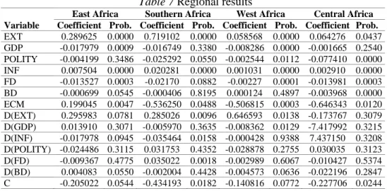
4.4.2. Regional Estimates
Although the PMG allows short-run estimates to differ across countries, the study split the sample into their distinct sub-region in the continent to assess whether the Pooled Mean Group estimates in both long- and the short run differ from the region. The results are reported in Table 7. External debt remains significant in all regions in the long run as well as in the short run except Central Africa, which has an insignificant relationship between external debt and capital flight in the short run even though it was significant in the long run. These results suggest a revolving door hypothesis in all sub-regions in Sub-Saharan Africa. In additions, political stability, financial development, budget deficit and inflation are all significant and have the aprori expected signs across the sub-region, in the long run, indicating that capital flight is very sensitive to financial development, political stability, inflation and budget deficit across all regions. This means that any instance of financial instability, political crisis, high levels of inflation and fiscal deficit in the HIPC countries will continue to produce high levels of capital flight.
5. Conclusion and policy implications of the study
This paper examined the relationship between capital flight and external debt in HIPC countries in Sub-Saharan Africa employing the Pooled Mean Group (PMG) estimator of Autoregressive Distributed Lag (ARDL) model for the period 1970 to 2012. The empirical evidence presented in this paper suggests that there is both short-run and long-run relationship between external debt and capital flight in Sub-Saharan Africa signifying that increases in external debt accumulation lead to increase in capital flight
Table 7 Regional results
Variable
East Africa Southern Africa West Africa Central Africa Coefficient Prob. Coefficient Prob. Coefficient Prob. Coefficient Prob.
EXT 0.289625 0.0000 0.719102 0.0000 0.058568 0.0000 0.064276 0.0437 GDP -0.017979 0.0009 -0.016749 0.3380 -0.008286 0.0000 -0.001665 0.2540 POLITY -0.004199 0.3486 -0.025292 0.0550 -0.002544 0.0112 -0.077410 0.0000 INF 0.007504 0.0000 0.020281 0.0000 0.001031 0.0000 0.002910 0.0000 FD -0.013527 0.0003 -0.02170 0.0882 -0.00227 0.0001 -0.013981 0.0003 BD -0.000699 0.0545 -0.000406 0.8195 0.000124 0.4897 -0.003968 0.0000 ECM 0.199045 0.0047 -0.536250 0.0488 -0.506815 0.0003 -0.646343 0.0120 D(EXT) 0.295983 0.0781 0.285026 0.0096 0.646593 0.0138 -0.173767 0.3079 D(GDP) 0.013910 0.3071 -0.005970 0.3635 -0.008362 0.0129 -7.417992 0.3215 D(INF) -0.017978 0.0945 -0.035464 0.0158 -0.000428 0.9388 7.437150 0.3208 D(POLITY) -0.024486 0.3115 0.031753 0.4352 -0.028878 0.2755 0.030035 0.3123 D(FD) -0.009367 0.4775 0.035022 0.0018 -0.002989 0.6067 -0.010427 0.5374 D(BD) 0.004083 0.0550 -0.002004 0.4428 -0.004573 0.0636 -0.022196 0.2847 C -0.205022 0.0544 -0.434193 0.0182 -0.140816 0.0772 -0.227706 0.0244 Source: Computed by the authors using Eviews 9