E Economic Exposure and Crisis Resilience in Exogenous Shock

(1)

E

Vivien Czeczeli – Pál Péter Kolozsi – Gábor Kutasi – Ádám Marton

Economic Exposure and Crisis Resilience in Exogenous Shock

The Short-Term Economic Impact of the Covid-19 Pandemic in the EU

Summary: The coronavirus epidemic arrived in Europe in the spring of 2020, causing a significant slowdown in economic activity.

The study examines the preparedness, vulnerability, exposure and performance of 25 European countries during the economic crisis caused by the Covid-19 epidemic. Countries can be divided into seven groups with the cluster analysis executed during the research, based on fiscal, social, and external vulnerability indicators. Specific patterns of country groups are explored in the value and evolution of crisis period indicators of production, labor market, mobility and risk premium. The aim of the analysis is to find a correlation between pre-crisis preparedness and the extent of the economic shock caused by the crisis. The research divided the countries into seven groups based on their fiscal and social stance and external vulnerability. Then, specific patterns of country groups are explored in the value and evolution of production, labour market, mobility and risk premium indicators during the crisis. The analysis concludes that a clear link can be established merely between the state of public finances and the indicator of financial risk in the examination of the behaviour of clusters. For all clusters, it was confirmed that the decline in mobility was mostly accompanied by a slowdown in industrial production, but not by unemployment, which may indicate the impact of economic policy measures aimed at maintaining jobs. The results support the initial theoretical assumption that in an economic crisis caused by a exogenous shock originated in non-economic factor, the explanatory power in terms of short-term effects is much lower than in crises caused by economic risks.

KeywordS: Covid-19, fiscal policy, crisis, cluster-analysis, EU JeL-codeS: C38, E60, H12, H60, J60

doI: https://doi.org/10.35551/PFQ_2020_3_1

Economic developments in 2020 have been fundamentally determined by the pandemic caused by the covid-19 virus and the public health and economic policy measures taken in

response. A decline in economic activity has been common in all affected countries, but its extent, process and structure has shown certain variations. The 2008 global economic crisis gives rise to the assumption that the condition and economic preparedness of individual countries are decisive factors for the process of a crisis. This study seeks to answer the following question: can the economic E-mail address: czeczeli.vivien@uni-nke.hu

kolozsi.pal.peter@uni-nke.hu kutasi.gabor@uni-nke.hu marton.adam@uni-nke.hu

(2)

differences associated with the coronavirus be related to the socio-economic situation of a country at the outbreak of the crisis, and can deviations be detected in the short-term output variables of the economic crisis based on such vulnerabilities?

In Europe, the economic crisis has been managed with a mix of basically similar economic policies (czeczeli et al., 2020), so we aim to explore phenomena that can be related to the grouping of countries. our study focuses on 25 European countries and is based on multidimensional clustering, in which the basis of group formation is the state of public finances (public debt and deficit), income distribution within society (social expenditures in the state budget and GINI indicator), external economic processes (export share), as well as exposure to tourism as a sector requiring mobility.

The behaviour of the clusters thus created is analysed using four short-term trend indicators: labour mobility, unemployment, industrial production and risk spread data.

In the last step of the analysis, it is examined to what extent the clusters moved in parallel in the short-term period before the crisis, and then to what extent they moved apart from one another, or possibly experienced similar trends, during the crisis. The position in terms of each variable is evaluated in the months before and during the crisis by means of standard deviation and correlation calculation. subsequently, the co-movement of crisis indicators and the resulting trends during the crisis period are analysed. our initial assumption is that there is a correlation between economic behaviour during the crisis and the state of public finances, income distribution and external vulnerabilities prior to the outbreak of the crisis.

The current study is to be the initial element of a complex analysis project that aims to understand the dynamics, correlations

and interactions of the coronavirus pandemic.

It is essentially relevant for our analysis that, in many cases, the data and time series necessary for drawing durable conclusions in-depth are not yet available, thus, our results can be considered as a first estimate. In the context of the certain impacts, further research is needed, but the correlations explored in this study may also help to define the direction of future research activities.

THEorETiCal baCkgroUnd

over the past decade, there has been a lively theoretical debate about the role of economic policy in connection with the 2008 global financial crisis, from which the Austrian school (Hayek, 1995) and the Keynesian theory (Keynes, 1936) emerged victorious with their intervention and stimulation approaches (szepesi, 2013; Lentner and Kolozsi, 2019;

Móczár, 2010; csaba, 2009). This became a cornerstone for crisis management and the rethinking of models, while the non-Keynesian fiscal policy based on friedman’s monetarist approach (friedman, 1977), stimulating consumption through austerity (feldstein, 1982; Alesina and Perotti, 1995; Perotti et al., 1998; schucknecht and Tanzi, 2005; Benczes, 2008), has been pushed out of the forefront of economic policy.

one of the characteristic features of the treatment of the 2020 coronavirus pandemic has been that, in contrast to 2008, as a result of the above, the theoretical search for appropriate methods did not delay interventions this time, the activist perception of the state has clearly remained dominant in the economic approaches. still, fiscal policy and economic theory have faced new challenges. The restrictions introduced due to the coronavirus are clearly to be interpreted as a drop in demand and thus as a negative

(3)

demand shock. How is a demand shock classically manifested in economic thinking?

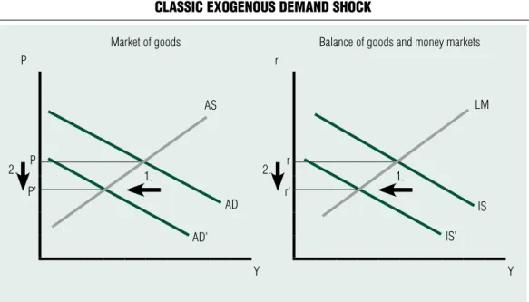
As a typical interpretation, consumption is lower at the same price level (meaning that the aggregate demand curve shifts to the left), and aggregate demand is lower at the same interest rate level (meaning that the Is curve shifts to the left) (see Figure 1). In such cases, the usual fiscal step is to replace lost private demand (household consumption, private investment) with higher government consumption, from reserves or from credit.

Various budgetary multiplicator calculations also provide a hint regarding the appropriate level of expenditure increase and tax reduction in such situations.

However, in the case of the coronavirus, the process of the exogenous demand shock is different: Households would be very happy to consume and companies would be ready to invest, but restrictions by the state and/

or caution (fear) impose a physical barrier to accessing services and products. consequently

in this case, processes can be appropriately modelled by breaking the demand or the Is curve, rather than by means of shifts in these curves (Figure 2). Thus, price and interest rate sensitivity do not change, only the consumed quantity is maximised, like in the case of the classic quantitative quota, only that demand is limited, rather than supply. fiscal policy is also not supposed to simply make up for lost demand, as it is in fact suppressed demand in this case. on the one hand, in the short term, the problem of time inconsistency must be managed, meaning that capacities or, from another perspective, sources of income must be, actually kept alive in order that demand can prevail again after cancellation of lockdown . on the other hand, in the long term, the state also has to contribute to the restructuring of the economy in order to avoid, to some extent, a repeated break in demand. If we accept that in the event of an epidemic, the demand shock works in the special way already described, then the Lucas critique of the ineffectiveness

Figure 1 ClassiC exogenous demand shoCk

market of goods balance of goods and money markets

P r

2. 2.

P’ r’

Y Y

Source: own edited

ad’

ad aS

1.

iS’

iS lm

1.

(4)

of economic policy (Lucas, 1976; sargent and Wallace, 1975; 1976) can also be ignored as the economy is not in a natural, long-term constant (stationary) equilibrium state of supply, but in a lower production level. In this situation, it would not be able to return to this level on its own on a market basis until the pandemic comes to an end. As the bankruptcy of companies, the loss of jobs and, ultimately, capacity drops and recoveries are not regulated by movements in supply and demand but by an exogenous factor, therefore, if the government leaves capacity owners alone, the economy may not be able to return to the original level of long-term equilibrium supply. That is why fiscal activism cannot be considered ineffective, even at a theoretical level.

At the same time, the covid-19 crisis cannot be interpreted narrowly, merely from the aspect of demand shock. The crisis describes an unusual combination of supply and demand shocks. In the modern monetary

system, this has been the first economic shock simultaneously reducing both supply and demand (Baqaee-farhi, 2020; shastri, 2020;

Bekaert et al. 2020). Therefore, negative demand-side impacts may be amplified by supply-side weaknesses. A sudden stop in manufacturing activities, along with the specificities of global value chains, deserve special attention in the current situation.

failing that, the absence of inputs may lead to a series of factory closures, which could also have spill-over effects in areas less affected by the virus. Production processes may collapse in countries that are more exposed to infected regions. Apart from production, the supply side is also affected by the reduction in labour supply (uNIDo, 2020). According to Bekaert et al. (2020), the distinction between supply and demand shocks is also important because the crisis management of negative demand and supply shocks requires very different forms on the fiscal and monetary sides. Aggregate demand shocks are defined Figure 2 suppressed demand shoCk due to the Coronavirus pandemiC

market of goods balance of goods and money markets

P r

Y Y

iS lm

ad aS

(5)

as ones that guide inflation and real activity in opposite directions. In contrast, demand shocks guide inflation and real activity in the same direction. The extent and nature of the shocks will be determined by developments in the coronavirus pandemic. In the event of a rapid decay, the supply shock will disappear quickly and production will recover soon.

The creation of the clusters presented in this study is justified by the fact that market economies and fiscal policies do not operate in exactly the same form, with identical institutions and processes (Hall and soskice, 2001; farkas, 2017). The approach separating European social models has already started to recognise this, which can also be regarded as a kind of classification of fiscal models as it classifies the quality of public taxes and expenditures and the level of the balance of the budget as distinguishing features (Boeri, 2002; Boeri and Baldi, 2005; sapir, 2005;

schubert and Martens, 2005; Bakács and Borkó, 2006). The following cluster analysis is based on a similar approach, aiming to make a distinction between economic models relevant to the crisis in the context of European market economies.

aPPliEd mETHodologY and daTa SoUrCES

studies based on the cluster analysis procedure aim to establish an initial framework. This group formation maps out the economic and social conditions at the end of 2019 in certain Member states of the European union.¹ It presents the economic situation that was characteristic of each country when the sARs- coV-2 (covid-19) virus, and the resulting economic impacts, reached a given country, as well as the resulting economic effects.

cluster analysis forms the basis of the analyses performed.

Cluster analysis

from among the grouping procedures, one of the most popular econometric methods is cluster analysis, which results in homogeneous groups based on various variables. The 27 European union Member states² under review can be considered a small sample, which led us to use hierarchical clustering on the database created. Grouping was based on 6 variables. Two of the variables represent fiscal policy conditions, two represent the exposure of each economy to tourism and exports, and two represent the social situation.

Each variable involved in the analysis can be measured on a metric measurement scale.

Accordingly, the Ward procedure was used for clustering. similarities between individual elements can be mapped out based on distance in the Ward procedure (simon, 2006). Within the framework of this analysis, distance was calculated using a square Euclidean distance as follows:

n

d(x,y)²=

∑

^(x^k^–y^k⁾²

k=1

The Ward procedure can be classified as a merging hierarchical clustering method.

During the merging process, based on the pre- calculated and aggregated distance values, the clusters with the lowest increase in variance within the cluster are merged. (sajtos and Mitev, 2007). The Ward method (and also the method of hierarchical clustering) is sensitive to outliers, which need to be filtered out before defining the clusters. This can be done using the shortest distance method (simon, 2006; sajtos and Mitev, 2007).

According to the survey conducted, Malta and Lithuania can be regarded as countries with outliers, so, for methodological reasons, these Member states may not be included in the database providing a basis for the cluster

(6)

analysis.³ A weak correlation can be detected between the variables involved in the analysis based on Pearson’s correlation coefficient, and, because these are macroeconomic variables, from a methodological perspective, cluster analysis can be performed on those variables.

Accordingly, in addition to the parameters described, the distance matrix of countries can be established, and individual clusters can be delimited.

After the clusters have been created, the economic indicators measured during the pandemic will be analysed in order to reveal differences and similarities between the groups of countries. During the analysis process, using data from the period between March-June 2020 for each cluster, a standard deviation and, for the co-movement of individual indicators, a correlation are calculated, and R² is also determined as an indicator for the strength of correlation. When revealing short-term impacts, the analysis approaches from four aspects. The pandemic and the restrictions were channelled into economic activity by changes in mobility, so this is the starting point. The result is a change in industrial production, as a measure of the degree of contraction in economic activity. This will be followed by developments in unemployment and changes in risk spread, reflecting financial risks.

Data

The cluster analysis was aimed to map out, as clearly as possible, the situation at the end of 2019 (in order to be able to study the short- term effects of the covid-19 pandemic in a complex manner, both between and within clusters). Nevertheless, the data and analysis projected for that period would not reflect the relevant macroeconomic relations and situation. Accordingly, trends in the processes of recent years were mapped out using various

simple statistical methods for each variable.

During the analyses, 2016 was used as a baseline year, while in the case of data for the year under review, a bottleneck was created by the availability of data in international databases. (In the case of indicators reflecting the social and societal situation, the latest data set available for the whole sample is represented by the values at the end of 2018.) The exact description of the variables may be as follows:

• average change in the balance of general government deficit (–) and surplus (+) over the period 2016-2019 - percentage;

• in the case of general government gross debt, the difference between 2016 and 2019 - percentage points;

• the difference of exports of goods and services, % of GDP between 2016 and 2019 - percentage points;

• travel and tourism total contribution to GDP, average of year-end data between 2016 and 2018 - percentage;

• share of cofoG - Gf10 - social protection expenditures, three-year average of year-end data between 2016 and 2018 - percentage;

• GINI indicator, three-year average of year-end data between 2016 and 2018 - percentage.

The analysis of clusters formed on the basis of historical data was continued using four indicators suitable for the identification of short-term impacts:

• industrial production,⁴ volume index of production, index 2015=100, change was included in the calculations - percentage,

• worker mobility, average of daily data, (based on Google covid-19 community mobility reports), as a percentage of the baseline value,

• unemployment rate - seasonally adjusted data, not calendar adjusted data, relative to the working age population - percentage,

(7)

• government bond spreads - percentage point.

Industrial production data on a monthly basis were identified using the relevant Eurostat indicator, which includes the fields of mining, quarrying, processing industry, electricity, gas, steam supply and air conditioning. The data series of industrial production is also a proxy indicator of developments in GDP, which allows monthly comparison with other data, as opposed to GDP change estimated by statistical offices over quarterly periods.

The change in mobility was quantified with the help of the Google community Mobility database. The data available here show to what extent people’s ‘movement’ deviates from the typical baseline value. The unemployment rate shows the ratio of the unemployed to the working age population as a percentage, based on the Eurostat database. Government bond spreads come from the Bloomberg database and show the values of the premiums of five- year bonds relative to German benchmark data.

In the second part of the empirical analysis, these indicators are used to identify the effects representing the developments of the months most severely affected since the beginning of the pandemic. our aim is to examine, based on the country groups created, whether any pattern can be identified in the outcome variables of the crisis caused by the pandemic based on the clusters arranged according to the economic, fiscal and social state before the crisis. In addition to providing a detailed picture of immediate economic responses that have been given in each country, the research identifies whether there is a correlation between the initial economic situation and the economic developments resulting from the shock caused by the pandemic. Detailed descriptive statistical data for each variable are included in Table 1.

Due to differences in scale size, the variables included in the cluster were standardised at z

value (z = ^x–μ_δ ) . The variables developed in the above manner provide a picture of economic and social relations in recent years in each country, and, furthermore, they reflect the state before the economic downturn caused by the lockdown due to the crisis.

rESUlTS

The result of clustering

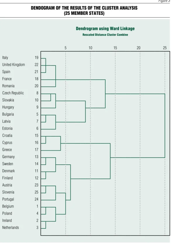
The number of clusters can be established in different ways: based on the relative size of clusters, the elbow criterion and the distances (sajtos and Mitev, 2007). The individual clusters were delimited taking all these considerations into account, and in an endeavour to form as homogeneous country groups as possible. The results of the studies are illustrated in the dendogram in Figure 3.

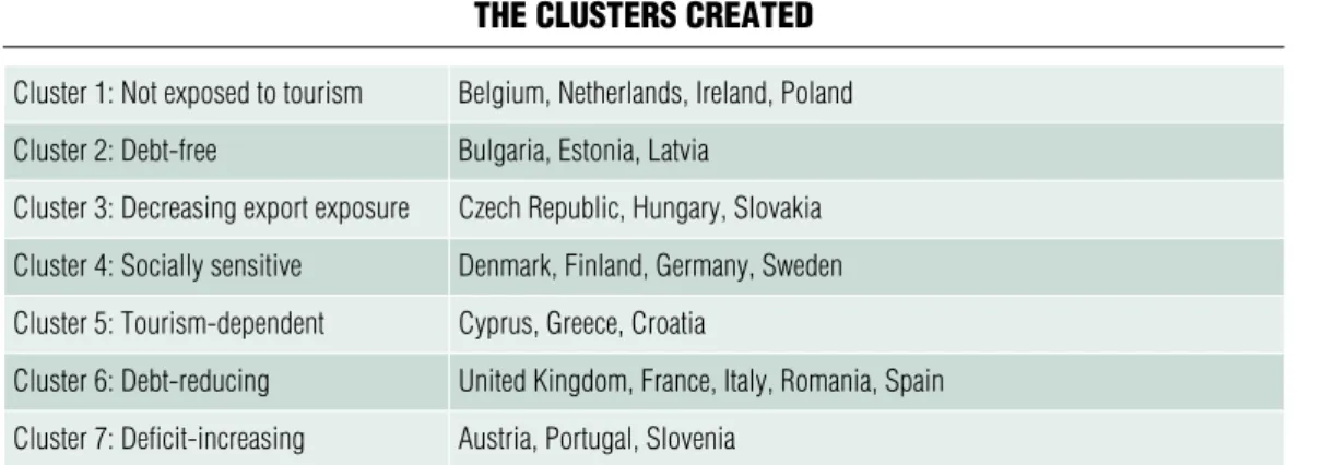
Based on the dendogram, it is possible to form several clusters with different numbers and numbers of items. In order to form the appropriate groups, it is necessary to examine the standard deviation of each group of countries to be formed in relation to the total standard deviation, i.e. the homogeneous nature of each cluster created. Based on the analyses, the version including seven clusters can be considered the most homogeneous, based on which we created seven groups. The assignment of the countries to the clusters is shown in Table 2.

As far as item numbers are concerned, groups of almost identical size, including 3, 4 and in one case 5 countries, were created. The clusters created are clearly separated from one another and reflect the macroeconomic and social situation in recent years.

Examining the differences between the individual clusters, it can be concluded that a surplus regarding the average balance of the budget was accumulated only by socially

(8)

Table 2 the Clusters Created

Cluster 1: not exposed to tourism belgium, netherlands, ireland, Poland Cluster 2: debt-free bulgaria, Estonia, latvia

Cluster 3: decreasing export exposure Czech republic, Hungary, Slovakia Cluster 4: Socially sensitive denmark, Finland, germany, Sweden Cluster 5: Tourism-dependent Cyprus, greece, Croatia

Cluster 6: debt-reducing United kingdom, France, italy, romania, Spain Cluster 7: deficit-increasing austria, Portugal, Slovenia

Note: the designations are to be understood as relative to other groups in each case Source: own calculation

Table 1 summary table of variables inCluded in the analysis extended

with desCriptive statistiCs

variable average standard

deviation minimum maximum data source Fiscal variables

average change of balance of the budget (as a percentage of gdP)

–0.71 1.4 –3.16 1.44 Eurostat

Change in gross consolidated public debt ratio –6.58 4.48 –15 0.1 Eurostat Variables representing economic exposure

Change in export share 1.79 3.15 –4.88 7.12 World bank

Travel and tourism average, total contribution to gdP

11.19 5.52 4.52 25 World bank

Indicators of societal and social situation average change in the rate of social expenditures (CoFog - gF10, as a percentage of gdP)

17.4 3.67 12.1 24.7 Eurostat

average of the gini indicator 29.79 3.92 22.8 39.17 Eurostat

Variables describing short-term effects

industrial production 100.66 14.5 59.4 132.7 Eurostat

mobility of people to work –35.97 13.65 –68.6 –13.67 google Community

mobility

Unemployment rate 6.24 3.07 2 16.2 Eurostat

government bond spread 1.75 2.53 0.01 13.17 bloomberg

Source: the authors’ own calculations based on Eurostat and World bank data

(9)

Figure 3 dendogram of the results of the Cluster analysis

(25 member states)

dendrogram using ward linkage

rescaled distance Cluster Combine

5 10 15 20 25

italy 19

United kingdom 22

Spain 21

France 18

romania 20

Czech republic 8

Slovakia 10

Hungary 9

bulgaria 5

latvia 7

Estonia 6

Croatia 15

Cyprus 16

greece 17

germany 13

Sweden 14

denmark 11

Finland 12

austria 23

Slovenia 25

Portugal 24

belgium 1

Poland 4

ireland 2

netherlands 3

Source: own figure using the SPSS program

(10)

sensitive countries and ones with a decreasing export exposure. The largest deficit was achieved by the countries of the debt-reducing and the relatively significant deficit-increasing cluster.

This trend can also be observed in the development of public debt, because debt- reducing countries have the lowest debt reduction in the period under review. fiscal discipline and the existence of structural imbalances may also play a significant role in this respect in the given group of countries.

In contrast, compared to debt-reducing countries, average debt reduction in the group not exposed to tourism increased nearly tenfold, while in the initial deficit-increasing cluster it increased nearly elevenfold between 2016 and 2019.

In the case of the indicator reflecting the change in export share, no significant differences can be identified; nevertheless, debt-free countries and ones with a decreasing export exposure, which also produced the highest per capita GDP growth, recorded a drop in export growth. However, this requires a detailed examination in order to be able to identify possible temporary changes and long- term trends. (This is done when identifying, characterising trends within each cluster).

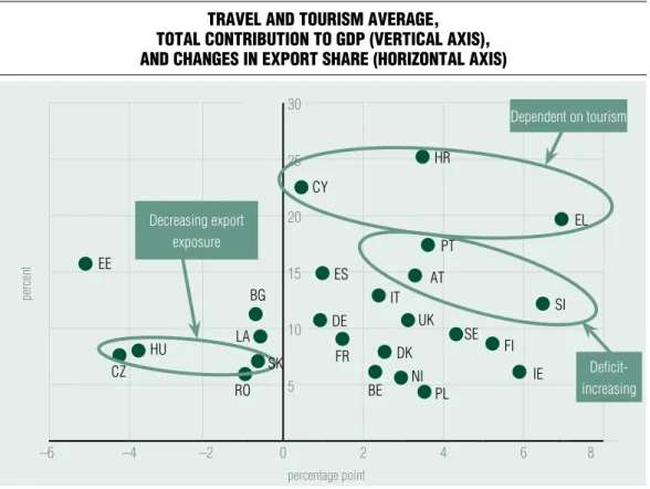
A review of the indicator reflecting the contribution of the travel and tourism sector to GDP also clearly reveals that the highest exposure is characteristic of countries depending on tourism. The weight of the tourism industry is not negligible either in the case of Italy, spain, the united Kingdom and france from cluster 6 and countries of cluster 7, i.e. Austria, Portugal and slovenia.

In terms of social expenditure, there is no significant difference between the groups of countries. The countries of the debt-free group deviate significantly from the overall sample, in a negative direction.

similarly, there is no significant difference in the GINI indicators. Two additional

variables were also included in the analysis, which will also be examined during the short- term cluster analysis. Based on year-end 2019 data, it can be concluded that unemployment rates are moderate (around 5 percent or lower) for most clusters, but the tourism-dependent and debt-reducing clusters are significantly different. for both clusters, cluster averages are considerably increased by indicators from southern European countries with structural problems and high youth unemployment like Greece (17.3 percent), Italy (10 percent) or spain (14.1 percent).

An analysis of per capita GDP growth shows that newly acceded Member states have higher growth rates (debt-free and with a decreasing export exposure) than the socially sensitive group with countries that are long- established members of the Eu. If individual clusters are examined by groups of variables, then the differences within each cluster can also be identified.

When forming the groups, fiscal variables can be considered key indicators in three clusters (Figure 4). These three clusters are the following: tourism-dependent, debt-reducing and deficit-increasing. The examination of all Member states makes it clear that the public debt ratio decreased everywhere between 2016 and 2019, except for two countries. In france, it increased by 0.1 percentage point, while in Italy it remained unchanged. However, taking the average development of budget balances into consideration, a more heterogeneous pattern emerges. In the period under review, partly as a positive consequence of economic trends, the average balance of the budget exceeded the Maastricht threshold of 3% only in Italy and spain. furthermore, 8 Member states experienced a surplus. This category includes the socially sensitive group, with the exception of finland, which is characterised by the effects of fiscal discipline and regulations.

When forming the groups, the indicators

(11)

describing external exposure became key group-forming criteria for 3 groups of countries: debt-free, tourism-dependent, and deficit-increasing (see Figure 5). from among the indicators describing external exposure, compared to the baseline year of 2016, a slight reduction in the change in export share is shown by the group of debt-free countries and those with a decreasing export exposure, as well as Romania. In the case of Estonia, the czech Republic and Hungary, which show the largest reduction, this change describes a typical trend for the last few years. In these countries, an ever lower share of the national income is generated by export activities. In many cases (e.g. Hungary), the share of export activities is still significant, but there is a gradual fall in the previously significant trade balance surplus. In other affected countries,

including Romania, the development of export share shows a relatively stable picture, with minor fluctuations. Looking at the countries of the debt-reducing group, the increase in export share is also moderate. In these countries, the contribution of exports to the GDP is approximately 30 percent, which is quite low, meaning that dependence on foreign markets (foreign demand) is more moderate. In contrast, the group not exposed to tourism typically has a high export share, so their sales revenues show a higher dependence on the economic situation of other countries.

The tourism sector represents a major source of employment, government revenues and foreign currency revenues for a number of developed and developing countries. since the virus virtually stopped all tourism-related activities, many countries have experienced a Figure 4 average Change in publiC debt (horizontal axis)

and in balanCe of the budget (vertiCal axis)

percent

2

–4 –3 –2 –1 0

1 2

–2 –4 –6 –8 –10 –12 –14 –16

percentage point Source: own figure based on Eurostat data

ES

debt-reducing

deficit-increasing

dependent on tourism ro

Fr iT

Uk

HU

bE

Pl

PT aT Si

Hr

CY bg

SE CZ

dk El

nl EE

la

iE Sk

Fi

(12)

significant decline in GDP as well as a large increase in the unemployment rate (uN, 2020). The group of countries most sensitive to revenues from tourism are tourism- dependent, debt-free and deficit-increasing countries. However, the countries not exposed to tourism and those with a decreasing export exposure are much less exposed to revenues from travel and tourism.

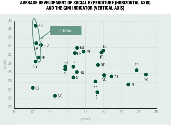
The GINI indicator, expressing income inequality, is the largest in the debt-free countries, meaning that inequality is the highest here (see Figure 6). The least favourable value was recorded in Bulgaria. As another characteristic of the country group, the share of social expenditures is the lowest here. As a result, the group of debt-free countries includes those with the highest inequality, as opposed to the lowest share of social expenditures.

Inequality is the lowest in countries with a decreasing export exposure. An important contribution to this fact is that slovakia and the czech Republic have the most favourable values among the countries reviewed. socially sensitive countries, the majority of which follow the model of the welfare state, as well as Germany, which can be described as a social market economy, and france, spend the largest amounts on social expenditures.

The former has a ratio of 12 percent, while in the case of latter, the value of the indicator is more than 20 percent. This means that the public care system and the social safety net are characterised by very different sizes in the individual countries.

Based on the average, minimum and maximum values of the cluster-forming variables illustrated in the group of Figures

Figure 5 travel and tourism average,

total Contribution to gdp (vertiCal axis), and Changes in export share (horizontal axis)

percent

30

25

20

15

10

5

–6 –4 –2 0 2 4 6 8

percentage point Source: own figure based on World bank data

ES decreasing export

exposure

deficit- increasing ro

Fr iT

Uk HU

bE Pl

aT PT Hr CY

bg

SE CZ

dk

El EE

la

Sk Fi

iE dE Si

ni

dependent on tourism

(13)

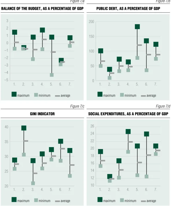
7 (balance of the budget, public debt, GINI indicator, social expenditures, share of tourism, export share), the following conclusions can be drawn.

As far as the balance of the budget is concerned, it is cluster 6 (debt-reducing countries) that differs the most with its higher deficit. from the point of view of budget balance averages, it is difficult to distinguish between the other six clusters. In terms of homogeneity, it is debt-reducing, debt-free (cluster 2) and deficit-increasing (cluster 7) countries that have a very strong internal coherence, and the three groups also take positions that can be easily distinguished from one another.

Regarding public debt, countries with a decreasing export exposure (group 3) and socially sensitive ones (group 4) take almost

identical positions with respect to both cluster average and low standard deviation (i.e. homogeneous composition). A similar observation can be made when comparing the averages of the debt-reducing and deficit- increasing groups, while the extreme values show a heterogeneous composition. cluster 2, made up of homogeneous debt-free countries, is markedly different from the others with its low debt ratio.

In the case of the GINI indicator, describing social exposure, the non-tourism- dependent cluster 1, the socially sensitive and the deficit-increasing countries produce similar averages, a distinction can only be made between them based on the group extremes. The other clusters are different from each other in terms of average, but it is only the non-tourism-dependent cluster and the

Figure 6 average development of soCial expenditure (horizontal axis)

and the gini indiCator (vertiCal axis) 40

percent

38 36 34 32 30 28 26 24 22 20

10 12 14 16 18 20 22 24 26

percent Source: own figure based on Eurostat data

ES debt-free ro

Fr iT

dE Uk

HU

bE Pl

PT

Si

aT CY Hr

bg

SE CZ

dk El

nl EE

la

iE

Sk

Fi

(14)

Figure 7 group behaviour of Cluster-forming variables, rate of variable (vertiCal axis),

Cluster number (horizontal axis)

Note: Horizontal axis: 1. - not exposed to tourism, 2. - debt-free, 3. - decreasing export exposure, 4. - socially sensitive, 5. - tourism- dependent, 6. - debt-reducing, 7. - deficit-increasing

Figure 7/a balanCe of the budget, as a perCentage of gdp

3 2 1 0 –1 –2 –3 –4

–5 1. 2. 3. 4. 5. 6. 7.

maximum minimum average

Figure 7/b publiC debt, as a perCentage of gdp 200

150

100

50

0 1. 2. 3. 4. 5. 6. 7.

Figure 7/c gini indiCator

40

35

30

25

20 1. 2. 3. 4. 5. 6. 7.

Figure 7/d soCial expenditures, as a perCentage of gdp

26 24 22 20 18 16 14 12

10 1. 2. 3. 4. 5. 6. 7.

(15)

tourism-dependent cluster (cluster 5) that can be considered relatively homogeneous.

There are marked differences in terms of average social expenditure. only the non- tourism-dependent cluster and the tourism- dependent countries have similar averages.

However, the clusters are characterised by very strong internal heterogeneity. only the debt- free countries are homogeneous, and only the deficit-increasing ones have a relatively small difference between their extreme values.

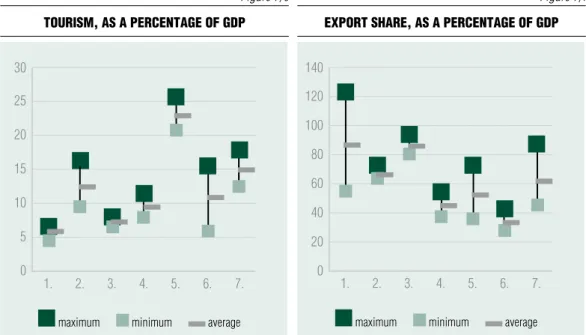
As far as exposure to tourism is concerned, most clusters are homogeneous or show a relatively small difference between extreme values (except debt-reducers), and their averages can be distinguished from one another. There is little overlap between the

clusters in terms of average export share as well; it is only countries not exposed to tourism and those with a decreasing export exposure that have nearly identical averages.

As regards homogeneity, the average is a good indicator of debt-free, tourism-dependent and socially sensitive countries, as well as debt- reducing ones.

Behaviour of clusters during the first wave of the virus

Based on the variation data detailed in Table 3, the clusters cannot be described as nearly homogeneous in terms of the time series characterising the four crisis periods. In some

Figure 7 group behaviour of Cluster-forming variables, rate of variable (vertiCal axis),

Cluster number (horizontal axis)

Figure 7/e tourism, as a perCentage of gdp

30 25 20 15 10 5

0 1. 2. 3. 4. 5. 6. 7.

Figure 7/f export share, as a perCentage of gdp

140 120 100 80 60 40 20

0 1. 2. 3. 4. 5. 6. 7.

(16)

months and for some indicators, however, certain clusters are well characterised by the cluster average. Examples include the change in industrial production for cluster 1 in April, clusters 3 and 6 in May, or, in addition to these two, cluster 5 in June. In the case of unemployment, there are clusters in March and April, whose countries hold together within the group, with the exception of clusters 5

and 6. In terms of mobility, however, only the April data of clusters 2 and 5 can be regarded as nearly homogeneous, while in the case of the government bond spread, clusters 2 and 4 behave like clusters.

Based on the analysis of the changes illustrated by the group of Figures 8, from the point of view of examining industrial production in the period before the crisis, Table 3 standard deviation of indiCators CharaCterising the Crisis period by Cluster

Cluster 1: not exposed to tourism Cluster 2: debt-free Cluster 3: decreasing export exposure Cluster 4: socially sensitive Cluster 5: tourism- dependent Cluster 6: debt- reducing Cluster 7: deficit- increasing

Change in industrial production

march 7.05 6.90 6.77 10.81 5.52 10.39 9.75

april 4.02 7.18 5.26 16.81 9.32 6.69 10.38

may 8.80 11.16 3.48 12.85 12.07 1.97 14.03

June 8.71 8.71 0.67 9.11 1.34 3.27 16.55

Unemployment

march 1.33 1.74 1.86 1.53 4.47 4.23 1.00

april 1.29 2.16 2.10 1.85 4.18 4.58 0.85

may 1.33 2.60 2.06 1.93 4.35 4.48 0.64

June 1.14 4.03 2.83 2.13 0.71 4.45 1.11

mobility

march 5.35 4.48 1.71 5.87 4.86 10.76 1.24

april 11.02 2.89 4.48 6.39 1.25 7.52 5.49

may 11.88 1.39 6.68 3.26 1.71 9.74 6.98

June 10.54 4.65 6.79 7.13 4.67 9.68 5.65

Change in government bond spread

2 January - 5 may 2020

0.38 0.11 0.69 0.07 0.55 0.44 0.29

Note: relatively low standard deviation is coloured by dark green Source: own calculation

(17)

Figure 8 group behaviour of variables indiCating a Crisis, rate of variable (vertiCal

axis), Cluster number (horizontal axis)

Source: own edited based on data from Eurostat, google Community mobility, bloomberg Figure 8/a

development of industrial produCtion in the four months before the Crisis (november 2019 - february 2020) and during the Crisis (marCh-June 2020)

145 135 125 115 105 95 85 75 65 55

1. (before) 1. (during) 2. (before) 2. (during) 3. (before) 3. (during) 4. (before) 4. (during) 5. (before) 5. (during) 6. (before) 6. (during) 7. (before) 7. (during) maximum (%) minimum (%) average (%)

Figure 8/b development of unemployment rate in the four months before the Crisis (november 2019 - february 2020) and during the Crisis (marCh-June 2020)

18 16 14 12 10 8 6 4 2 0

1. (before) 1. (during) 2. (before) 2. (during) 3. (before) 3. (during) 4. (before) 4. (during) 5. (before) 5. (during) 6. (before) 6. (during) 7. (before) 7. (during) maximum (%) minimum (%) average (%) Figure 8/c

workforCe mobility in the period before the Crisis (15-29 february 2020) and during the Crisis (marCh-June 2020)

60 40 20 0 –20 –40 –60 –80 –100

Figure 8/d government bond yields in the period before the Crisis (2 January

2020) and during the Crisis (7 may 2020)

4,5 4,0 3,5 3,0 2,5 2,0 1,5 1,0 0,5 0

(18)

individual cluster averages varied from 105 to 115 percent, which assumes a relatively homogeneous state. Within the clusters, the debt-free and debt-reducing countries, as well as those with a decreasing export exposure can be considered homogeneous, while the non- tourism-dependent and tourism-dependent groups are characterised by greater fluctuations.

During the period of the crisis, however, countries show larger variations within a group.

In all clusters, industrial production decreased to a different extent. As for the averages, the reduction of the indicator was smaller in the group of non-tourism-dependent, debt-free, socially sensitive and tourism-dependent countries, and it is especially the debt-free and socially sensitive groups where the change in the minimum value lowered the average. In the case of the other clusters created, the degree of decline was higher.

As far as the unemployment indicator is concerned, a more heterogeneous pattern emerged between the individual clusters even in the pre-crisis period. The tourism- dependent and debt-reducing countries had considerably higher average unemployment rates than the other country groups, but this can be attributed to the exceptionally high

outlier values. The crisis did not result in higher-than-average unemployment in most of the countries; however, the maximum values shifted, especially in the group of debt- free countries. furthermore, in the tourism- dependent countries, the maximum value even shows a drop. In addition, the difference in extreme values did not change significantly.

Workforce mobility shows the most heterogeneous picture before and after the crisis. cluster averages show similar reductions from similar levels. As another common phenomenon, the difference between the extreme values of the clusters has increased sharply.

Regarding the risk spread on government bond yields, there has been a general increase, but the degree thereof showed significant differences. While the risk premium remained stable in the countries not exposed to tourism, average interest rate premiums in debt-free, tourism-dependent and deficit-increasing countries rose relatively sharply. for the latter two clusters, homogeneity also fell significantly, as shown by the difference in extreme values.

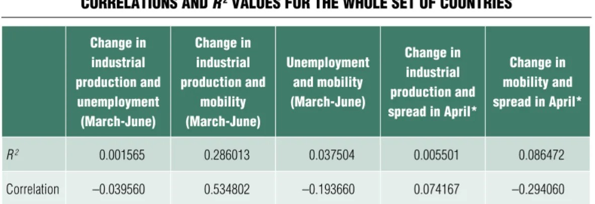
correlation data (see Table 4) suggest that there is no relevant statistical correlation

Table 4 Correlations and R ² values for the whole set of Countries

Change in industrial production and unemployment (march-June)

Change in industrial production and

mobility (march-June)

unemployment and mobility (march-June)

Change in industrial production and spread in april*

Change in mobility and spread in april*

R ² 0.001565 0.286013 0.037504 0.005501 0.086472

Correlation –0.039560 0.534802 –0.193660 0.074167 –0.294060

Note:* change in government bond spread (2 January - 5 may 2020) Source: own calculation

(19)

between unemployment and change in industrial production (compared to the same period of the previous year). Based on correlation data and the minimum value of R² describing the closeness of the relationship, unemployment is not closely related to the decline in mobility, either. Therefore, it is not relevant to examine the co-movement of these indicators. However, it is justified to examine the relationship between industrial production and mobility, as the correlation indicator between the two is 0.545, and R², describing the strength of fit of the linear trend function, explains the relationship between the two with a two-digit figure (28.6 percent). Therefore, the relationship between these two values will be analysed below by cluster.

In the case of the risk spread of government bonds, the difference between 2 January and 5 May 2020 was taken into account, so correlation with the April data, before 5 May, was calculated for the other data.

No co-movement can be detected with unemployment. There is minimum correlation with industrial production, while R² has almost zero explanatory power. It is only the reverse co-movement compared to the drop in mobility that deserves special attention (correlation: –0.294; R ²: 0.0865).

The group of Figures 9 shows a set of graphs describing industrial production and mobility:

in all clusters, the drop in mobility occurred in parallel with the slowdown in industrial production. Assuming that mobility is a kind of proxy for public health measures, co- movement is intuitive, as more substantial public health constraints result in a drop in industrial production (of course, due to the international nature of industry, it may be justified to examine industrial trends in the light of the data of trading partners, but the integration of these aspects is beyond the scope of this study). It is visible that mobility fell dramatically in April, with a considerable

correction in most countries by May, and the debt-free group, as well as the czech Republic and Hungary from the cluster with a decreasing export exposure, and the majority of countries belonging to the group not exposed to tourism returned to the March level by June (mobility data is missing from slovakia). cluster-level peculiarities can again be detected. cluster 2 can be described as one experiencing a minimum loss of mobility and a return to the positive domain. cluster 3 shows fully co- movement for both variables, but industrial production did not even reach the previous year’s level by June. (The Polish economy

‘stands out’ from the group with a decreasing export exposure as - although the Polish curve has a similar shape - the change in industrial production returned to an exceptionally high level of growth in June.)

In several countries, depending on the date of announcement of the pandemic, March data still show increasing industrial production and production is increasing again in June, i.e.

it does not merely indicate a decreasing level of reduction (compared to the same month of 2019). In finland and Denmark, production did not even fall into the negative domain.

However, the other half of cluster 4 shows a less homogeneous movement. sweden failed to converge to the starting point in March in terms of mobility and production. Germany was successful in this respect, but its industrial production was still significantly lower than a year before. (In the case of Greece and slovenia, industrial production decreased only to a minimum extent in April, and from May its change returned to the positive domain again on an annual basis. At the same time, the Dutch, Portuguese and swedish economies failed to return to the positive domain by June.) As a peculiarity of the tourism- dependent countries of cluster 5, mobility compared to the starting point was in the positive domain throughout the period, and

(20)

Figure 9 Co-movements in the time series of Clusters

in terms of mobility (horizontal axis)

and Changes in industrial produCtion (vertiCal axis) (marCh-June 2020)

Note: The captions for the dots include two letters as a country code, while the second two numbers represent the month of the year 2020.

For example, iT04 represents the april 2020 data of italy.

Figure 9/b debt-free (Cluster 2)

20 15 10 5 0 –5 –10 –15 –50 –40 –30 –20 –10 –0

la05

la04 EE03

EE04 EE05

bg03

bg06 bg04 bg05

la03 la06 Figure 9/a

not exposed to tourism (Cluster 1)

20 15 10 5 0 –5 –10 –15 bE04

–80 –60 –40 –20 –0 iE04

nl05

iE05

Pl03 Pl06

Pl04 bE05

Pl05 nl03

nl06 bE03bE06

nl04

iE03

iE06

Figure 9/c deCreasing export exposure (Cluster 3)

10 5 0 –5 –10 –15 –20 –25 –30 –50 –40 –30 –20 –10 –0

HU03

HU04

HU05

HU06 CZ06

CZ05

CZ04

CZ03

Figure 9/d soCially sensitive (Cluster 4)

20 15 10 5 0 –5 –10 –15 –20 –25 –30 –50 –40 –30 –20 –10 –0

Fi03

dk03

dk04 dk05 dk06

SE03

SE04 dE03

dE04

dE05 dE06 SE05 SE06

Fi04 Fi05

Fi06

(21)

Figure 9 Co-movements in the time series of Clusters

in terms of mobility (horizontal axis)

and Changes in industrial produCtion (vertiCal axis) (marCh-June 2020)

Note: The captions for the dots include two letters as a country code, while the second two numbers represent the month of the year 2020.

For example, iT04 represents the april 2020 data of italy.

Figure 9/e tourism-dependent (Cluster 5)

20 15 10 5 0 –5 –10 –15 –20 –25

CY05

CY04 CY03

0 5 10 15 El03

Hr03

Hr04 Hr05 Hr06 El04

El05 El06

Figure 9/f defiCit-inCreasing (Cluster 7)

20 15 10 5 0 –5 –10 –15 –20 –25 –30 Si03

aT03

PT03

PT04

PT05 aT04 PT06

aT05 aT06 Si04

Si05

Si06

–80 –60 –40 –20 –0

Figure 9/g debt-reduCing (Cluster 6)

5 0 –5 –10 –15 –20 –25 –30 –35 –40 –45 –80 –70 –60 –50 –40 –30 –20 –10 0

ro03

ro04 Fr04

Fr06

ES04

ES06 Uk03

Uk04

Uk05

Uk06

iT03

iT04

iT05 ro05

ro06

Fr05 Fr03

iT06 ES03

ES05

(22)

industrial production fell sharply only in April on an annual basis, and all three countries were able to return to growing production.

As a peculiarity of cluster 6, all countries belonging to the debt-reducing group show very wide variations, compared to the others, both in terms of job travel fluctuation (mobility) and declining industrial production. The former is in the range of (–20; –70), while the latter is in the range of 25-30 percentage points over the four months reviewed. cluster 5 shows a mixed picture with respect to industrial production, but there are a lot of similarities in the development of mobility, not only within the group, but also with debt-free countries and ones with a decreasing export exposure. cluster 1 is really heterogeneous, and it would be difficult to

make a general statement here in the context of production and mobility.

The correlation illustrated in Figure 10 suggests that no far-reaching conclusions can be drawn from the relationship between changes in the risk spread of government bonds and the fall in mobility, but in some cases it is possible to recognise the clusters identified from pre-crisis data. The socially sensitive cluster is clearly described by the characteristics of low risk spread and a 30- 45% drop in mobility. The Netherlands is also close to this group based on these two criteria.

The members of the debt-free group are also close to one another (Bulgaria and Latvia - no data for Estonia, as it has very little debt, and no 5-year debt at all). The croatian and Greek members of the tourism-dependent group

Figure 10 ConneCtions between Changes in government bond spreads

(2 January - 5 may 2020, horizontal axis) and mobility (vertiCal axis)

–20 –25 –30 –35 –40 –45 –50 –55 –60 –65 –70

Source: own edited data based on data from bloomberg, google

debt-reducing Socially sensitive

ES ro

Fr iT

Uk

HU

bE Pl

PT

Si

aT Hr

bg SE

CZ

dk

El nl

dE la

iE Fi

–1,0 –0,5 0 0,5 1,0 1,5 2,0

debt-free

dependent on tourism

(23)

suffered a similar degree of mobility drop (–52 per cent and –54 percent, respectively), but they show a significant difference in interest spread, presumably due to their crisis- independent public finance situation (see figure 4). countries in the debt-reducing cluster also show the same mobility drop with minimum standard deviation, with the exception of Romania, but similarly to Ireland, which is, however, in another cluster. However, their interest spreads appear to be basically determined by the debt trajectory, rather than the 2020 crisis. for the other clusters, it is not possible to identify such a markedly different position compared to the others in the context of risk spread and mobility.

Based on the monthly change in unemployment, there is a significant standard variation within the clusters in terms of both the degree of change and its development over time, so the clusters based on preparedness data before the crisis cannot be distinguished with respect to labour market impact. This is not surprising since many of the countries reviewed distorted market processes through job retention measures (see czeczeli et al., 2020) and, furthermore, unemployment statistics are necessarily based on administrative rules. However, it can be generally concluded that the closure already increased unemployment in April at the latest.

lESSonS and ConClUSionS

During the analysis, our starting point was a modified theory, which adapted the New Keynesian theory of economic policy to the peculiarities of the global economic crisis caused by the pandemic. This gave rise to the conclusion that, due to the inevitable drop in mobility, it is not enough to merely replace household consumption with public expenditure, but it is also necessary to focus on maintaining capacity.

The methodology of the study was based on Ward clustering and a coherent analysis of short-term variables. using the method of clustering, seven groups, each containing 3 to 5 countries, were defined based on six economic indicators that measure the vulnerability and exposure of the countries with respect to public finances, external economy and income distribution (i.e. social aspects) before the economic crisis. The groups of countries thus formed showed some similarities, as expected, but surprises were also found compared to the traditional versions of capitalism and the classic literature of European social models.

When examining cluster-forming variables, it was concluded that the clusters are clearly separable in the pair of social indicators. As for the other four indicators describing the initial situation before the crisis, the separation of the seven clusters is not so marked. As far as the budget deficit is concerned, cluster 6 stood out and deviated significantly in the direction of a deficit, while cluster 5 was unique due to a significant deviation of extreme values. With respect to public debt, the clusters can be divided into two types: clusters 2-4 typically entered the pandemic with lower levels of debt, clusters 5-7 with a higher level, while cluster 1 swayed between the two. The examination of export share also resulted in a similar division:

it was high in groups 1-3 and considerably lower in groups 4-7. In terms of exposure to tourism, only cluster 5 and cluster 1 are different from the other five, more or less homogenous groups of countries with a higher and lower share of GDP, respectively.

The defined clusters were analysed for the first four months of the pandemic, March- June 2020, based on four indicators that characterise a short period and that can be quickly realised statistically:



monthly change in industrial production compared to the same period of the previous year,