PUBLIC DEBT AND ECONOMIC GROWTH: FURTHER EVIDENCE FOR THE EURO AREA*

(1)

PUBLIC DEBT AND ECONOMIC GROWTH:

FURTHER EVIDENCE FOR THE EURO AREA

^*

Marta GÓMEZ-PUIG – Simón SOSVILLA-RIVERO

(Received: 29 September 2016; revision received: 24 April 2017;

accepted: 8 September 2017)

This paper empirically investigates the short and the long run impact of public debt on economic growth. We use annual data from both the central and the peripheral countries of the euro area (EA) for the 1961–2013 period and estimate a production function augmented with a debt stock term by applying the Autoregressive Distributed Lag (ARDL) bounds testing approach. Our results suggest different patterns across the EA countries and tend to support the view that public debt always has a negative impact on the long-run performance of EA member states, whilst its short-run effect may be positive depending on the country.

Keywords: public debt, economic growth, bounds testing, euro area, peripheral euro area countries, central euro area countries.

JEL classifi cation indices: C22, F33, H63, O40, O52

* This paper is based upon our work supported by the Instituto de Estudios Fiscales (Grant no. IEF 101/2014 and IEF 015/2017), the Banco de España (Grant no. PR71/15-20229), the Spanish Ministry of Education, Culture and Sport (Grant no. PRX16/00261) and the Span- ish Ministry of Economy and Competitiveness (Grant no. ECO2016-76203-C2-2-P). Simón Sosvilla-Rivero thanks the members of the Department of Economics at the University of Bath for their hospitality during his research visit. Responsibility for any remaining errors rests with the authors.

Simón Sosvilla-Rivero, corresponding author. Professor at the Department of Economic Analysis, Universidad Complutense de Madrid, Spain. E-mail: sosvilla@ccee.ucm.es

Marta Gómez-Puig, Associate Professor at the Department of Economics and Riskcenter, Universitat de Barcelona, Spain. E-mail: marta.gomezpuig@ub.edu

(2)

1. INTRODUCTION

The origin of the sovereign debt crisis in the euro area (EA) goes deeper than the fiscal imbalances in the member states. Some authors have pointed out that the EA faced three interlocking crises – banking, sovereign debt, and economic growth – which together challenged the viability of the currency union. Despite its relevance, an analysis of the interrelationship between sovereign and banking risk is beyond the scope of this paper. Rather, since the crisis led to an unprecedented increase in sovereign debt in the EA countries¹ we will focus on the interconnection between sovereign debt and growth in 11 of them, both the central (Austria, Belgium, Finland, France, Germany and the Netherlands) and the peripheral member states (Greece, Ireland, Italy, Portugal, and Spain). There is a widespread consensus on the potentially adverse consequences of high levels of public debt for these countries’ economic growth, but few macroeconomic policy debates have caused as much disagreement as the current austerity argument.

Overall, the theoretical literature favours the study of the effects of very high debt on the capital stock, growth, and risk, since it tends to point to a negative link between the public debt to Gross Domestic Product (GDP) ratio and the steady-state growth rate of GDP (Aizenman et al. 2007). The literature also high- lights that the impact of debt on output may differ depending on the time horizon − while debt may crowd out capital and reduce output in the long run, in the short run it can stimulate aggregate demand and output (Barro 1990; Elmendorf – Mankiw 1999; Salotti – Trecroci 2016). Further, it stresses that the presence of a tipping point, above which an increase in public debt has a detrimental effect on economic performance, does not mean that it has to be common across countries (Ghosh et al. 2013 or Eberhardt – Presbitero 2015). The latter authors indicate that there may be at least three reasons for the differences in the relationships between public debt and growth across countries: (1) production technology may differ; (2) the capacity to tolerate high levels of debt may depend on a number of country-specific characteristics related to the macro and the institutional framework; and (3) the vulnerability to public debt may depend not only on the debt levels, but also on the debt composition.

Nevertheless, although the relevance of heterogeneity of the debt-growth nexus (both across countries and time periods) has been stressed by literature, and although certain authors have presented empirical analyses of this issue, hardly any empirical studies have examined the topic in the EA countries. While there is a substantial body of research exploring the interconnection between debt and

1 By the end of 2013, on average, public debt reached about 100% of GDP in the EA countries – its highest level in 50 years.

(3)

growth in both the developed and the emerging countries, few papers to date have looked at this link in the context of the EA. These exceptions make use of the panel data techniques to obtain average results for the EA countries, and do not distinguish between the countries or between the short and the long run effects.

In this context, this paper presents a new approach to add to the as yet small body of literature on the relationship between public debt accumulation and economic performance in the EA countries, by examining the potential heterogeneity in the debt-growth nexus both across different countries and time horizons.

Therefore, our contribution to the empirical literature is twofold. First, unlike previous studies, we do not make use of the panel estimation techniques to com- bine the power of cross section on average with all the subtleties of temporal dependence; rather, we explore the time series dimension of the issue to obtain further evidence based on the historical experiences of each country in the sample in order to detect potential heterogeneities in the relationship across these countries. Second, our econometric methodology is data-driven, and it allows us to select the statistical model that best approximates the relationship between the variables under this study for any particular country and to assess both the short and the long-run effects of public debt on output performance.

The rest of the paper is organised as follows. Section 2 justifies our empirical approach on the basis of a review of the existing literature. Section 3 presents the analytical framework of the analysis and outlines the econometric methodology.

Section 4 describes our data. Empirical results are presented in Section 5. Finally, Section 6 summarises the findings and offers some concluding remarks.

2. LITERATURE REVIEW

Under what conditions is debt growth-enhancing? This challenging question has been studied by economists for a long time, but has recently undergone a notable revival fuelled by the substantial deterioration of public finances in many economies as a result of the financial and the economic crisis of 2008–2009.

From the theoretical perspective, there is no consensus regarding the sign of the impact of public debt on output either in the short or the long run. The “conventional” view (Elmendorf – Mankiw 1999) states that in the short run, since output is demand-determined, government debt (manifesting deficit financing) can have a positive effect on disposable income, aggregate demand, and overall output. Moderate levels of debt are found to have a positive short-run impact on economic growth through a range of channels: improved monetary policy, strengthened institutions, enhanced private savings, deepened financial interme- diation (Abbas – Christensen 2010) or smoothed distortionary taxation over time

(4)

(Barro 1979). This positive short-run effect of budget deficits (and higher debt) is likely to be large when the output is far from full capacity. However, things are different in the long run if the decrease in public savings caused by a higher budget deficit and is not fully compensated by an increase in private savings. In this situation, both national savings and total investment will fall; this will have a negative effect on GDP as it will reduce capital stock, increase interest rates, and reduce labour productivity and wages. The negative effect of an increase in public debt on future GDP can be amplified if high public debt increases uncertainty or leads to expectations of future confiscation, possibly through inflation and financial repression (Cochrane 2011).

The above “conventional” split between the short and the long-run effects of debt disregards the fact that protracted recessions may reduce future potential output (as they increase the number of discouraged workers, with the associated loss of skills, and have a negative effect on organisational capital and investment in new activities). There is, in fact, evidence that recessions have a permanent effect on the level of future GDP (e.g. Cerra – Saxena 2008), which implies that running fiscal deficits (and increasing debt) may have a positive effect on output in both the short and the long run. DeLong –Summers (2012) argue that, in a low interest rate environment, an expansionary fiscal policy is likely to be self- financing.

Finally, another strand of literature also departs from the “conventional” view and establishes a link between the long-term effect of debt and the kind of public expenditure it funds. The papers by Aschauer (1989) and Devarajan et al. (1996), for instance, state that in the long run, the impact of debt on the economy’s performance depends on whether the public expenditure funded by government debt is productive or unproductive. Whilst the former (which includes physical infra- structure such as roads and railways, communication, information systems such as phone, internet, and education) may have a positive impact on the economy’s growth, the latter does not affect its long-run performance, although it may have positive short-run implications.

From the empirical perspective, the results from the literature on the relationship between public debt and economic growth are far from conclusive (either Panizza – Presbitero (2013) or the technical Appendix in Eberhardt – Presbitero (2015) for two excellent summaries of this literature). Some authors (Reinhart – Rogoff 2010 or Pattillo et al. 2011) present empirical evidence indicating that the relationship is described by an inverted U-shaped pattern (low levels of public debt positively affect economic growth, but high levels have a negative impact).

However, other empirical studies reach very different conclusions. While some of them find no evidence for a robust effect of debt on growth (Lof – Malinen 2014),

(5)

others detect an inverse relationship between the two variables (Woo – Koomar 2015) or contend that the relationship between them is mitigated crucially by the quality of a country’s institutions (Kourtellos et al. 2013).

In the EA context, when leverage was already very high, the recent economic recession and the sovereign debt crisis have stimulated an intense debate both on the effectiveness of fiscal policies and on the possible adverse consequences of the accumulation of public debt in the EA countries. Few macroeconomic policy debates have generated as much controversy as the current austerity argument, not only because pundits draw widely different conclusions for macroeconomic policy, but also because economists have not reached a consensus (Alesina et al.

2015). Some suggest that now is precisely the time to apply the lessons learnt during the Great Depression and that policymakers should implement expansionary fiscal policies (Krugman 2011 or DeLong – Summers 2012) since fiscal austerity may have been the main culprit for the recessions experienced by the European countries. Others argue that, since the high level of public sector leverage has a negative effect on economic growth, fiscal consolidation is fun- damental to restoring the confidence and improving the expectations about the future evolution of the economy and therefore its rate of growth (Cochrane 2011 or Teles – Mussolini 2014).

Few papers have examined the relationship between debt and growth for the EA countries despite the effects of the severe sovereign debt crisis in several member states. Checherita-Westphal – Rother (2012) and Baum et al. (2013) ana- lyse the non-linearities of the debt-growth nexus estimating a standard growth model and employing a panel approach. In contrast, Dreger – Reimers (2013) base their analysis on the distinction between sustainable and non-sustainable debt periods. Overall, this empirical literature lends support to the presence of a common debt threshold across the (similar) countries like those in the EA, and does not distinguish between the short and the long-run effects.

Therefore, to our knowledge, no strong case has yet been made for analysing the effect of debt accumulation on economic growth taking into account the particular characteristics of each EA economy and examining whether the effects differ depending on the time horizon, in spite of the fact that this potential heterogeneity has been stressed by the literature. For instance, Eberhardt – Presbitero (2015) and Égert (2015) support the existence of nonlinearity in the debt-growth nexus, but state that there is no evidence at all for a common threshold level to all countries over time. Gómez-Puig – Sosvilla-Rivero (2015) and Donayre –Taivan (2017) also suggest that the causal link is intrinsic to each country.

(6)

3. ANALYTICAL FRAMEWORK AND ECONOMETRIC METHODOLOGY An important line of research, based on the empirical growth literature (e.g. Barro – Sala-i-Martin 2004), has considered growth regressions augmented by public debt to assess whether the latter has an impact on growth over and above other determinants, such as population growth, human capital, financial development, innovation intensity, openness to trade, fiscal indicators, saving or investment rate and macroeconomic uncertainty (e.g. Cecchetti et al. 2011; Pattillo et al.

2011; Checherita-Westphal – Rother 2012).

Our empirical strategy departs from this approach and explores the debt–

growth nexus using an aggregate production function augmented by debt. This allows us to test the impact of debt after controlling for the basic drivers of growth:

the stock of physical capital, the labour input and a measure of human capital.

The stock of physical capital and the labour input have been the two key determinants of economic growth since Solow’s neoclassical model (1956) and many empirical studies have examined their relationship with economic growth (e.g.

Frankel 1962). Regarding human capital, Becker (1962) stated that the investment in human capital contributed to economic growth by investing in people through education and health, and Mankiw et al. (1992) augmented the Solow model by including accumulation of human as well as physical capital (Savvide – Stengos 2009).

Therefore, we extend Eberhardt – Presbitero’s (2015) approach and consider the following aggregate production function, in which public debt is included as a separate factor of production²:

( , , , )

t t t t t

Y  AF K L H D (1)

where Y is the level of output, A is an index of technological progress, K is the stock of physical capital, L is the labour input, H is the human capital, and D is the stock of public debt.

For simplicity, the technology is assumed to be of the Cobb-Douglas form:

3

1 2 4

t t t t t

Y  AK L H D^α ^α ^α ^α (2) so that, after taking logs and denominating the log terms by small letters of its corresponding capital letters, we obtain

1 2 3 4 .

t t t t t

y  α αk α l α h α d ₍₃₎

2 Eberhardt – Presbitero (2015) do not consider H in the basic equation of interest for their analysis of the debt–growth nexus.

(7)

As can be seen, equation (3) postulates a long-run relationship between (the log of) the level of production (y_t), (the log of) the stock of physical capital (k_t), (the log of) the labour employed (l_t), (the log of) the human capital (h_t) and (the log of) the stock of public debt (d_t). In contrast to Eberhardt – Presbitero (2015), we do not impose any constraint in the production function regarding the returns to scale of production factors.

Equation (3) can be estimated from sufficiently long-time series using cointegration techniques. In this paper, we make use of the Autoregressive Distributed Lag (ARDL) bounds testing approach to the cointegration proposed by Pesaran – Shin (1999) and Pesaran et al. (2001). This approach presents at least three significant advantages over the two common alternatives used in the empirical literature: the single-equation procedure developed by Engle – Granger (1987) and the maximum likelihood method based on a system of equations postulated by Johansen (1991, 1995). First, both these approaches require the variables under study to be integrated of order 1; this inevitably requires a previous process of tests on the order of integration of the series, which may lead to some uncertainty in the analysis of long-run relations. In contrast, the ARDL bounds testing approach allows the analysis of long-term relationships between variables, regardless of whether they are integrated of order 0 [I(0)], of order 1 [I(1)] or mutually cointe- grated. This avoids some of the common pitfalls faced in the time series analysis, such as the lack of power of unit root tests and doubts about the order of integration of the variables examined (Pesaran et al. 2001). Second, the ARDL bounds testing approach allows a distinction to be made between the dependent variable and the explanatory variables, an obvious advantage over the method proposed by Engle – Granger. At the same time, like the Johansen approach, it allows si- multaneous estimation of the short-run and long-run components, eliminating the problems associated with omitted variables and the presence of autocorrelation.

Finally, while the estimation results obtained by the methods proposed by Engle – Granger and Johansen are not robust to small samples, Pesaran – Shin (1999) show that the short-run parameters estimated using their approach are √T consistent and that the long-run parameters are super-consistent in small samples.

In our particular case, the application of the ARDL approach to cointegration involves estimating the following unrestricted error correction model (UECM):

3

1 2 4

1 1 1 1 1

1 1 2 1 3 1 4 1 5 1

q q q q

p

t i t i i t i i t i i t i i t i

i i i i i

t t t t t t

y y k l h d

y k l h d

β γ ω φ υ

λ λ λ λ λ ε

    

    

    

            

     

    

^ ₍₄₎

where Δ denotes the first difference operator, β is the drift component, and ε_t is assumed to be a white noise process. Note that p is the number of lags of the

(8)

dependent variable and q_i is the number of lags of the i-th explanatory variable.

The optimal lag structure of the first differenced regression (4) is selected by the Akaike Information Criterion (AIC) and the Schwarz Bayesian Criterion (SBC) to simultaneously correct for the residual serial correlation and the problem of endogenous regressors (Pesaran – Shin 1999: 386). In order to determine the existence of a long-run relationship between the variables under study, Pesaran et al. (2001) propose two alternative tests. First, an F-statistic is used to test the joint significance of the first lag of the variables in levels (i.e. λ₁ λ₂ λ₃ λ₄ λ₅ 0), and then a t-statistic is used to test the individual significance of the lagged dependent variable in levels (i.e. λ₁ = 0).

Based on two sets of critical values: I(0) and I(1) (Pesaran et al. 2001), if the calculated F- and/or t-statistics exceed the upper bound I(1), we conclude in favour of a long-run relationship, regardless of the order of integration. However, if these statistics are below the lower bound I(0), the null hypothesis of no cointegration cannot be rejected. Finally, if the calculated F- and/or t-statistics fall between the lower and the upper bound, the results are inconclusive.

If the cointegration exists, the conditional long-run model is derived from the reduced form equation (4) when the series in first differences are jointly equal to zero (i.e., Δy = Δk = Δl = Δd = 0). The calculation of these estimated long-run coefficients is given by:

1 2 3 4 5 .

t t t t t t

y  δ δ k δ l δ h δ d ξ (5) Finally, if a long-run relation is found, an error correction representation exists and it is estimated from the following reduced form equation:

3

1 2 4

1 1 1 1 1 1

1 1 1 1 1

q

q q q

p

t i t i t i t i t i t t

i i i i i

y θ y_ k_ π l_ τ h_ ψ d_ ηECM_

    

 



 



^  



 



 



 

(6)

4. DATA

We estimate equation (4) with the annual data for eleven EA countries: both the central (Austria, Belgium, Finland, France, Germany and the Netherlands) and the peripheral countries (Greece, Ireland, Italy, Portugal and Spain). Even though the ARDL-based estimation procedure used in the paper can be reliably used in small samples, we use long spans of data covering the period 1961–2013 (i.e. a total of 52 annual observations) to explore the dimension of historical specificity and to capture the long-run relationship associated with the concept of cointegration (e. g. Hakkio – Rush 1991).

(9)

To maintain as much homogeneity as possible for a sample of 11 countries over the course of five decades, our primary source is the European Commission´s AMECO database³. We then strengthen our data with the use of supplementary data sourced from IMF (International Financial Statistics) and the World Bank (World Development Indicators). We use GDP, net capital stock and public debt (all expressed at 2010 market prices) for Y, K and D, respectively, as well as civil- ian employment and life expectancy at birth for L and H⁴ respectively.

5. EMPIRICAL RESULTS⁵

5.1. Time series properties

Before carrying out the ARDL cointegration exercise, we test for the order of integration of the variables using the Augmented Dickey-Fuller (ADF) tests. This is necessary just to ensure that none of our variables are stationary at second differences, since the ARDL bounds test fails to provide robust results in the presence of I(2) variables. The results decisively reject the null hypothesis of non-stationarity, suggesting that all variables can be treated as first-difference stationary⁶.

3 http://ec.europa.eu/economy_finance/db_indicators/ameco/index_en.htm

4 Following Sachs – Warner (1997), we use life expectancy at birth as a proxy for human capital. Other commonly used proxies for human capital, such as years of secondary education, enrolment at secondary school and measures of human capital using a Mincerian equation (e.

g. Morrisson – Murtin 2007) were available at homogeneous form for all EA countries under study starting from 1980. Additionally, years of secondary education did not change during the sample period. As shown in Jayachandran – Lleras-Muney (2009), longer life expectancy encourages human capital accumulation, since a longer time horizon increases the value of investments that pay out over time. Moreover, better health and greater education are comple- mentary with longer life expectancy (Becker 2007). We also considered the index of human capital per person provided by the Penn World Table (version 8.0, Feenstra et al. 2013), based on years of schooling (Barro – Lee 2013) and returns to education (Psacharopoulos 1994).

This index is only available until 2011 and, for the countries under study, is a I(2) variable that cannot be included in our analysis. Nevertheless, life expectancy at birth correlates strongly with the index of human capital per person during the 1961–2011 period.

5 We summarise the results by pointing out the main regularities and focusing on public debt.

The reader is asked to browse through Tables 1 and 2 to find evidence for a particular country of her/his special interest.

6 These results (not shown here in order to save space, but available from the authors upon request) were confirmed using Phillips-Perron (1998) unit root tests controlling for serial correlation and the Elliott et al. (1996) Point Optimal and Ng – Perron (2001) unit root tests for testing non-stationarity against the alternative of high persistence. These additional results are also available from the authors upon request.

(10)

Then, following Cheung – Chinn’s (1997) suggestion, we confirm these results using the Kwiatkowski et al. (1992) (KPSS) tests, where the null is a stationary process against the alternative of a unit root⁷.

The single order of integration of the variables encourages the application of the ARDL bounds testing approach to examine the long-run relationship between the variables.

5.2. Empirical results from the ARDL bounds test

The estimation proceeds in stages. In the first stage, we specify the optimal lag length for the model (in this stage, we impose the same number of lags on all variables as in Pesaran et al. 2001). The ARDL representation does not require sym- metry of lag lengths; each variable may have a different number of lag terms. As mentioned above, we use AIC and SBC to make our choice of the lag length, se- lecting 4 as the maximum number of lags both for the dependent variable and the regressors. For the test of serial correlation in the residual, we use the maximum likelihood statistics for the first and fourth autocorrelation, denoted as χ²_SC(1) and χ²_SC(4), respectively. Due to constraints of space, these results are not shown here but they are available from the authors upon request.

Next, we test for the existence of a long-run relation between the output and its components, as suggested by equation (3).

Panel A in Table 1 gives the values of the F- and t-statistics for the case of unrestricted intercepts and no trends (case III in Pesaran et al. 2001)⁸. These statistics are compared with the critical value bounds provided in Tables CI and CII of Pesaran et al. (2001) and depend on whether an intercept and/or trend is included in the estimations. This suggests the existence of a single long-term relationship in which the production level would be the dependent variable and the stock of physical capital, the labour employed, the human capital and the stock of public

7 The results are not shown here due to space limit but are available from the authors upon request.

8 Since the hypothesis of the expected values of the first differences of the series to be zero cannot be rejected, there is no evidence of linear deterministic trends in the data. Therefore, we conclude that the cointegrating relationship should be formulated with the constant term unrestricted and without deterministic trend terms (case III). Nevertheless, we also consider two additional scenarios for the deterministics: unrestricted intercepts, restricted trends; and unrestricted intercepts, unrestricted trends (cases IV and V in Pesaran et al. 2001). These additional results are not shown here due to space constraints, but they are available from the authors upon request. Our estimation results indicate that the intercepts are always statistically significant, whereas the trends are not.

(11)

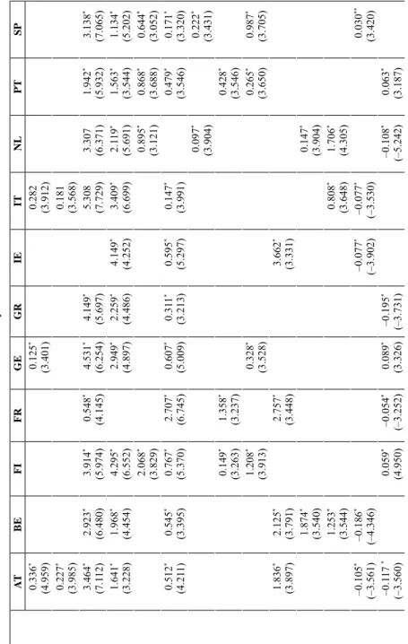
Table 1. Long-run analysis Panel A: Bound testing to cointegration ATBEFIFRGEGRIEITNLPTSP ARDL(p,q1,q2,q3,q4,q5)(4, 3, 3, 4, 4)(1, 2, 4, 4, 0)(1, 4, 3, 1, 2)(1, 0, 2, 4, 3)(2, 2, 1, 0, 2)(1, 3, 0, 0, 0)(1, 2, 1, 0, 0)(3, 2, 0, 4, 1)(1, 4, 3, 4, 4)(1, 3, 3, 0, 2)(1, 3, 2, 0, 3) F-statistic6.815*5.045**5.035**4.163**6.007*4.509**4.612**5.396*6.773*4.323**4.350** t-statistic–5.291*–3.709**–3.822**–3.868**–4.702*–3.695**–3.744**–3.628**–4.286*–3.860**–4.064** Panel B: Long-run coefficients ATBEFIFRGEGRIEITNLPTSP Intercept 0.412* (3.033)0.398* (3.214)0.363* (3.561)0.450* (3.621)0.463* (3.021)0.155* (3.021)0.274* (2.997)0.232* (3.143)0.322* (3.055)0.174* (3.034)0.162* (3.051) kt0.296* (6.628)0.396* (6.071)0.426* (5.665)0.429* (5.826)0.497* (5.488)0.245* (5.488)0.232* (6.172)0.312* (5.843)0.444* (6.287)0.330* (4.204)0.489* (7.400) lt 0.328* (6.176)0.452* (7.788)0.411* (7.292)0.428* (3.835)0.520* (3.483)0.312* (3.483)0.395* (3.531)0.472* (6.375)0.358* (6.320)0.373* (2.942)0.324* (4.040) ht0.085* (2.892)0.421* (2.978)0.538* (4.138)0.507* (3.998)0.584* (2.932)0.346* (2.932)0.131* (3.124)0.142* (3.723)0.357* (4.198)0.205* (2.947)0.353* (3.395) dt–0.129* (–4.335)–0.062* (–5.512)–0.049* (–5.137)–0.544* (–5.867)–0.040* (–3.135)–0.079* (–3.135)–0.049* (–7.783)–0.083* (–6.723)–0.097* (–7.318)–0.354* (–6.336)–0.336* (–4.871) Notes: AT, BE, FI, FR, GE, GR, IE, IT, NL, PT and SP stand for Austria, Belgium, Finland, France, Germany, Greece, Ireland, Italy, the Netherlands, Portugal and Spain, respectively. In Panel A, p, q1, q2, q3, q4 andq5denote, respectively, the optimal lag length for ∆yt-i, ∆kt-i, ∆lt-i, ∆ht-i and ∆dt-i in the UECM model (4) without deterministic trend; * and ** indicate that the calculated F- and t-statistics are above the upper critical bound at 1% and 5%, respectively. In Panel B, in the ordinary brackets below the parameter estimates, the corresponding t-statistics are shown; * denotes statistical significance at the 1% level.

(12)

debt would be the independent variables. Then, the estimated long-run relationships between the variables are reported in Panel B in Table 1.

Some very interesting results can be drawn from the empirical evidence presented in Table 1. First, as it registers a negative value in all EA countries, the long-term effect of debt on economic performance is in line with the findings of previous empirical literature based on panel data techniques. However, the magnitude of the negative impact differs significantly across the countries, implying that our conclusions need to be qualified. While comparatively high impacts are estimated in the case of France (–0.544), Portugal (–0.354), Spain (–0.336), and Austria (–0.129), in the rest of the countries, although negative, the magnitude is very small with values close to zero. Ireland (–0.049), Finland (–0.049) and Germany (–0.040) are the countries with the lowest negative impact.

Therefore, our results suggest that, even though debt has a long run negative impact on output in all EA countries, with the exception of France, Portugal, Spain and Austria its magnitude is negligible.

In order to examine the short-term dynamics of the model, we estimate an ECM associated with the above long-run relationship. As can be seen in Table 2, the short-run impact of debt on economic performance differs clearly across the countries, both in terms of the estimated coefficients for Δd_t and in terms of the significance of lagged terms of Δd_t. In order to compare results, we fol- low Hendry ’s (1995) suggestion and calculate the short-term effects of debt on growth as follows for the significant coefficients:

short-term effects ⁴

1 1

/ (1 )

q p

i i

ψ θ

 







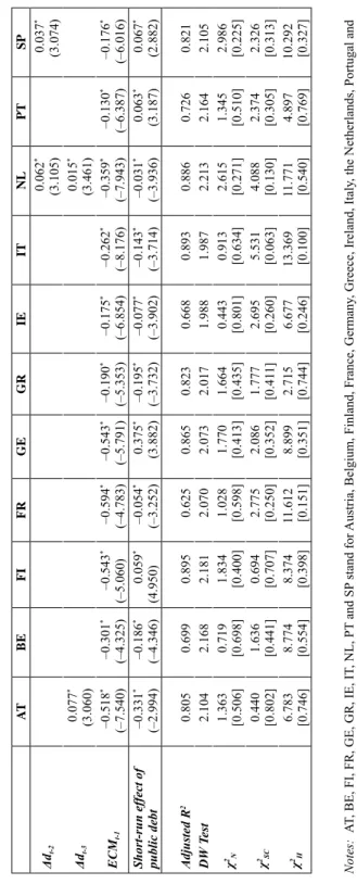
⁽⁷⁾

Table 2 shows that with respect to the peripheral EA countries, in spite of the important long-run negative impact in Portugal and Spain, the short-term effect is positive (0.063 and 0.067), although quite small. However, in Greece, Ireland and Italy an increase in public debt has a negative effect on GDP, not only in the long run but in the short run as well. Among the central EA countries, it is noticeable that in Germany and Finland the effect of public debt on GDP is positive in the short run (0.375 and 0.059) despite the negative (though very small) effect in the long run. Finally, in the cases of Austria, Belgium, France and the Netherlands our results suggest that public debt has a negative impact on economic activity in both the short and the long run.

All in all, it should be noted that we do not find a positive long-run relationship between public debt and output in any country, although the short-run link is positive in four EA countries. Interestingly, in two peripheral countries, Spain and Portugal, while debt exerts an important negative effect on the long run, its impact, although small, is positive in the short run. These results are in

(13)

Table 2. Short-run analysis ATBEFIFRGEGRIEITNLPTSP Δyt-10.336* (4.959) 0.125* (3.401) 0.282 (3.912) Δyt-20.227* (3.985) 0.181 (3.568) Δkt3.464* (7.112)2.923* (6.480)3.914* (5.974)0.548* (4.145)4.531* (6.254)4.149* (5.697)5.308 (7.729)3.307 (6.371)1.942* (5.932)3.138* (7.065) Δkt-11.641* (3.228) 1.968* (4.454)4.295* (6.552)2.949* (4.897)2.259* (4.486)4.149* (4.252)3.409* (6.699)2.119* (5.691)1.563* (3.544)1.134* (5.202) Δkt-2 2.068* (3.829) 0.895* (3.121) 0.868* (3.688) 0.644* (3.052) Δlt 0.512* (4.211)0.545* (3.395)0.767* (5.370)2.707* (6.745)0.607* (5.009) 0.311* (3.213)0.595* (5.297)0.147* (3.991)0.479* (3.546) 0.171* (3.320) Δlt-1 0.097* (3.904)0.222* (3.431) Δlt-20.149* (3.263)1.358* (3.237) 0.428* (3.546) Δht1.208* (3.913)0.328* (3.528) 0.265* (3.650)0.987* (3.705) Δht-11.836* (3.897)2.125* (3.791)2.757* (3.448) 3.662* (3.331) Δht-21.874* (3.540) 0.147* (3.904) Δht-31.253* (3.544) 0.808* (3.648)1.706* (4.305) Δdt–0.105* (–3.561)–0.186* (–4.346) –0.077* (–3.902)–0.077* (–3.530) 0.030** (3.420) Δdt-1–0.117 * (–3.560)0.059* (4.950)–0.054* (–3.252)0.089* (3.326) –0.195* (–3.731) –0.108* (–5.242)0.063* (3.187)

(14)

ATBEFIFRGEGRIEITNLPTSP Δdt-2 0.062* (3.105)0.037* (3.074) Δdt-30.077* (3.060) 0.015* (3.461) ECMt-1–0.518* (–7.540)–0.301* (–4.325)–0.543* (–5.060)–0.594* (–4.783)–0.543* (–5.791) –0.190* (–5.353)–0.175* (–6.854)–0.262* (–8.176)–0.359* (–7.943)–0.130* (–6.387)–0.176* (–6.016) Short-run effect of public debt–0.331* (–2.994)–0.186* (–4.346)0.059* (4.950)–0.054* (–3.252)0.375* (3.882)–0.195* (–3.732)–0.077* (–3.902)–0.143* (–3.714)–0.031* (–3.936)0.063* (3.187)0.067* (2.882) Adjusted R20.8050.6990.8950.6250.8650.8230.6680.8930.8860.7260.821 DW Test2.1042.1682.1812.0702.0732.0171.9881.9872.2132.1642.105 χ^{2 N}1.363 [0.506]0.719 [0.698]1.834 [0.400]1.028 [0.598]1.770 [0.413]1.664 [0.435]0.443 [0.801]0.913 [0.634]2.615 [0.271]1.345 [0.510]2.986 [0.225] χ^{2 SC}0.440 [0.802]1.636 [0.441]0.694 [0.707]2.775 [0.250]2.086 [0.352]1.777 [0.411]2.695 [0.260]5.531 [0.063]4.088 [0.130]2.374 [0.305]2.326 [0.313] χ^{2 H}6.783 [0.746]8.774 [0.554]8.374 [0.398]11.612 [0.151]8.899 [0.351]2.715 [0.744]6.677 [0.246]13.369 [0.100]11.771 [0.540]4.897 [0.769]10.292 [0.327] Notes:AT, BE, FI, FR, GE, GR, IE, IT, NL, PT and SP stand for Austria, Belgium, Finland, France, Germany, Greece, Ireland, Italy, the Netherlands, Portugal and Spain, respectively; In the ordinary brackets below the parameter estimates, the corresponding t-statistics are shown. The short-run effects of public debt are calculated using equation (7); * and ** denote statistical significance at the 1% and 5% level, respectively. χ^{2 N,}χ^{2 SC}and χ^{2 H}are the Jarque-Bera test for normality, the Breusch-Godfrey LM test for second-order serial correlation and the Breusch-Pagan-Godfrey test for het- eroskedasticity. In the square brackets, the associated probability values are given.

Table 2. cont.

(15)

line with some recent literature which has investigated how different country characteristics (e.g. the state of the public finances, the health of the financial sector or the degree of openness to trade) might influence the size of fiscal multipliers. In particular, Corsetti et al. (2012) and Ilzetzki et al. (2013) find that negative multipliers can be observed in the high-debt countries (i.e., with debt-to-GDP ratios above 60%), but they could be much larger in the countries under sound public finances. Furthermore, Eberhart – Presbitero (2015) stress that one of the reasons that explains the differences in the relationships between public debt and growth across countries is the dependence of vulnerability to public debt on current debt levels. Among the peripheral EA countries, only Portugal and Spain registered an average debt ratio below the 60% threshold during the 1961–2013 period (37% and 35%, respectively), while the debt ratio was also moderate in Finland and Germany (28% and 40%, respectively, on average). Therefore, our results confirm that in the countries with low or moderate indebtedness levels (i.e., in a sustainable public debt context, see Dreger – Reiners 2013), an additional increase in public debt might exert a short-run positive effect on GDP.

These findings are highly relevant since these two peripheral countries have been hit especially hard by both the economic and sovereign debt crises. And, amid the crisis, they received rescue packages (in the Spanish case, to save its banking sector) which were conditional on the implementation of structural reforms to improve competitiveness and highly controversial fiscal austerity measures (whose positive effects are nevertheless typically related to the long-run).

Although our results must be regarded with caution since they present the average effects over the 50-year estimated period, they do not seem to favour the same austerity argument in all EA countries. In particular, they indicate that, in the short term, the expansionary fiscal policies may not have a negative effect on output – but a marginal positive one − in some countries such as Spain and Por- tugal, regardless of its large negative impact in the long run. Then, although our findings support the view that the unprecedented sovereign debt levels in the EA countries might have adverse consequences for their economies in the long run, they also suggest that the pace of adjustment may differ across these countries. In particular, within the peripheral EA countries, policymakers should bear in mind that while the short-run impact of debt on economic performance is negative in Greece, Ireland and Italy, it is slightly positive in Spain and Portugal.

Regarding the estimated coefficients for the ECM_t-1 representing the speed of adjustment needed to restore equilibrium in the dynamic model following a dis- turbance, Table 2 shows that they range from –0.301 to –0.594 in the central countries (suggesting that, with the exception of Belgium and the Netherlands, more than half of the disequilibrium is corrected within one year), while ranging from –0.129 to –0.262 in the peripheral EA countries (suggesting relatively slow

(16)

reactions to deviations from equilibrium and implying that short-term effects may dominate at longer horizons). Besides, the highly significant estimated ECM_t-1 provide further support for the existence of stable long-run relationships such as those reported in Table 1 (Banerjee et al. 1998).

As Table 2 indicates, the short-run analysis seems to pass diagnostic tests such as normality of error term, second-order residual autocorrelation and heteroske- dasticity (χ²_N,χ²_SCand χ²_H, respectively). The regressions fit reasonably well, with R² values ranging from 0.625 for France to 0.895 for Finland.

The estimated parameters presented in Table 2 are average values for the entire sample period (1961–2013) and do not take into account the possibility that they could change over time if a structural break occurred⁹. Therefore, we also explore the possibility of multiple structural changes in the parameter relating the public debt variable to the real growth rate (ψ_t) in equation (6) by using the Bai – Perron (1998) test. The results (not shown here to save space, but available from the authors upon request) seem to strongly suggest that there are two structural breaks in each of the estimated models. Re-estimating the regression model including a dummy variable that incorporates the detected breakpoints and gauge whether structural breaks have disturbed the effect of public debt on the real growth rate, we find very different results across the countries. Regarding the central EA countries, with the exception of France, where debt had a negative short-run effect on growth (Austria, Belgium, and the Netherlands), these inverse relationships between debt and growth seem to strengthen throughout the detected regimes.

However, in Germany and Finland (where debt had a positive short-run effect on growth), we only detect a positive relationship between these two variables during the first regime (i.e., before the first break point). Subsequently, debt also exerts a negative effect on growth in Germany and Finland, respectively¹⁰. All in all, our results seem to suggest that the debt-to-GDP ratio at which public debt exerts the strongest negative impact on economic growth changes over time and across the EA countries.

6. CONCLUDING REMARKS

Despite the severe sovereign debt crisis in the EA, few papers have examined the relationship between debt and growth for the EA countries. The literature available lends support to the presence of a common debt threshold across the EA

9 We are grateful to an anonymous referee for suggesting this analysis.

10 These additional results are not shown here because of space limit, but they are available from the authors upon request.

(17)

countries but does not distinguish between the short and the long-run effects. To our knowledge, no strong case has yet been made for analysing the incidence of debt accumulation on economic growth taking into account the particular characteristics of each EA economy and examining whether the effects differ depending on the time horizon, even though this potential heterogeneity has been stressed by the literature.

This paper aims to fill this gap. Unlike previous studies in the EA, we do not make use of panel techniques but study cross-country differences in the debt- growth nexus across the EA countries over time horizons using time series analyses. To this end, our empirical examination of 11 countries (both the central and the peripheral) during the 1961–2013 period is based on the estimation of a log- linearised Cobb-Douglas production function augmented with a debt stock term for each country, by means of the ARDL testing approach to cointegration.

As in every empirical analysis, the results must be regarded with caution since they are based on a set of countries over a certain period and a given econometric methodology. This is particularly true for the comparison of the results with those of previous papers, since we adopt a time series analysis instead of a panel data approach; and since we use an analytical framework based on a production function augmented with public debt instead of growth regressions augmented by public debt. Nonetheless, our findings are in concordance with the predomi- nant view that the positive effect of debt on output is more likely to be felt in the short rather than in the long run. In particular, our empirical evidence suggests a negative effect of public debt on output in the long run. Thus, our results support the previous reports indicating that high public debt tends to hamper growth by increasing uncertainty over future taxation, crowding out private investment, and weakening a country’s resilience to shocks (e.g. Krugman 1988). However, they detect the possibility that an increase in public debt may have a positive effect in the short run by raising the economy’s productive capacity and improving ef- ficiency depending on the characteristics of the country and the final allocation of public debt. Specifically, this short-run positive effect is found in Finland, Ger- many, Portugal and Spain, suggesting that in a context of low rates of economic growth, the path of fiscal consolidation may differ across the EA countries.

This issue is particularly relevant to policymakers because of its implications for the effectiveness of a common fiscal policy, in view of the pronounced differences in the responsiveness of output in the long and the short run and across the countries. These findings seem to corroborate the idea that there is no “one size fits all” definition for fiscal space but that, debt limits and fiscal space may be country-specific and depend on each country’s track record of adjustment (e. g.

Ostry et al. 2010).

(18)

Extensions from the present research might take a number of directions. First, it would be interesting to examine possible non-linear effects (smooth or sud- den structural changes) using the time-series approach to detect further potential heterogeneities among the EA countries, complementing the evidence from existing literature using the panel data techniques. A second natural extension to the analysis presented in this paper would be to further explore the main determinants of the detected differences in the relationships between public debt and economic growth across the countries, with special emphasis on the economic and institutional factors. Both items are on our future research agenda.

REFERENCES

Abbas, S. M. A. – Christesen, J. E. (2010): The Role of Domestic Debt Markets in Economic Growth: An Empirical Investigation for Low-Income Countries and Emerging Markets. IMF Staff Papers, 57(1): 209–255.

Alesina, A. – Barbiero, O. – Favero, C. – Giavazzi, F. – Paradisi, M. (2015): Austerity in 2009- 2013. Economic Policy, 30(83): 383–437.

Aizenman, J. – Kletzer, K. – Pinto, B. (2007): Economic Growth with Constraints on Tax Revenues and Public Debt: Implications for Fiscal Policy and Cross-Country Differences. Working Paper, No. 12750, Cambridge, MA: National Bureau of Economic Research.

Aschauer, D. A. (1989): Is Public Expenditure Productive? Journal of Monetary Economics, 23(2):

177–200.

Bai, J. – Perron, P. (1998): Estimating and Testing Linear Models with Multiple Structural Changes.

Econometrica, 66(1): 47–78.

Baier, S. L. – Glomm, G (2001): Long-Run Growth and Welfare Effects of Public Policies with Distortionary Taxation. Journal of Economic Dynamics and Control, 25(12): 2007–2042.

Banerjee, A. – Dolado, J. – Mestre, R. (1998): Error-Correction Mechanism Tests for Cointegration in a Single-Equation Framework. Journal of Time Series Analysis, 19(3): 267–283.

Barro, R. J. (1979): On the Determination of the Public Debt. Journal of Political Economy, 87(5):

940–971.

Barro, R. J. (1990): Government Spending in a Simple Model of Endogenous Growth. Journal of Political Economy, 98(5): S103–S125.

Barro, R. – Lee, J. W. (2013): A New Data Set of Educational Attainment in the World, 1950-2010.

Journal of Development Economics, 104(C): 184–198.

Baum, A. – Checherita-Westphal, C. – Rother, P. (2013): Debt and Growth: New Evidence for the Euro Area. Journal of International Money and Finance, 32: 809–821.

Becker, G. S. (1962): Investment in Human Capital: A Theoretical Analysis. Journal of Political Economy, 70(2): 9–49.

Becker, G. S. (2007): Health as Human Capital: Synthesis and Extensions. Oxford Economic Papers, 59(3): 379–410.

Cecchetti, S. – Mohanty, M. S. – Zampolli, F. (2011): Achieving Growth Amid Fiscal Imbalances:

The Real Effects of Debt. In: Achieving Maximum Long-Run Growth, pp. 145–196. Symposium at Jackson Hole: Federal Reserve Bank of Kansas City.

Cerra, V. – Saxena, S. C. (2008): Growth Dynamics: The Myth of Economic Recovery. American Economic Review, 98(1): 439–57.

(19)

Checherita-Westphal, C. – Rother, P. (2012): The Impact of High Government Debt on Economic Growth and its Channels: An Empirical Investigation for the Euro Area. European Economic Review, 56(7): 1392–1405.

Cheung, Y.-W. – Chinn, M. D. (1997): Further Investigation of the Uncertain Unit Root in GNP.

Journal of Business and Economic Statistics, 15(1): 68–73.

Cochrane, J. H. (2011): Understanding Policy in the Great Recession: Some Unpleasant Fiscal Arithmetic. European Economic Review, 55(1): 2–30.

Corsetti, G. – Roubini, N. (1991): Fiscal Defi cits, Public Debt and Government Solvency: Evidence from OECD Countries. Journal of the Japanese and International Economies, 5(4): 354-380.

Cottarelli, C. – Jaramillo, L. (2013): Walking Hand in Hand: Fiscal Policy and Growth in Advanced Economies. Review of Economics and Institutions, 4(2):1–25.

De Hek, P. A. (2006): On Taxation in a Two-Sector Endogenous Growth Model with Endogenous Labor Supply. Journal of Economic Dynamics and Control, 30(4): 655–685.

Delong, J. B. – Summers, L. H. (2012): Fiscal Policy in a Depressed Economy. Brookings Papers on Economic Activity (Spring), 233–274.

Devarajan, S. – Swaroop, V. – Zou, H. G. (1996): The Composition of Public Expenditure and Economic Growth. Journal of Monetary Economics, 37(2): 313–344.

Donayre, L. – Taivan, A. (2017): Causality between Public Debt and Real Growth in the OECD:

A Country-by-Country Analysis. Economic Papers, 36(6): 156–170.

Dreger, C. – Reimers, H. E. (2013): Does Euro Area Membership Affect the Relation between GDP Growth and Public Debt? Journal of Macroeconomics, 38(B): 481–486.

Eberhardt, M. – Presbitero, A. F. (2015): Public Debt and Growth: Heterogeneity and Non-Linearity.

Journal of International Economics, 97(1): 45–58.

Égert, B. (2015): The 90% Public Debt Threshold: The Rise and Fall of a Stylised Fact. Applied Economics, 47(34-35): 3756–3770.

Elmendorf, D. W. – Mankiw, N. G. (1999): Government Debt. In: Taylor, J. B. – Woodford, M.

(eds): Handbook of Macroeconomics, Vol. 1C, pp. 1615–1669. Amsterdam: North-Holland.

Elliott, G. – Rothenberg, T. J. – Stock, J. H. (1996): Effi cient Tests for an Autoregressive Unit Root.

Econometrica, 64(4): 813–836.

Engle, R. F. – Granger, C. W. J. (1987): Co-Integration and Error Correction: Representation, Estimation and Testing. Econometrica, 55(2): 251–276.

Feenstra, R. C. – Inklaar, R. – Timmer, M. P. (2013): The Next Generation of the Penn World Table.

www.Ggdc.Net/Pwt.

Frankel, M. (1962): The Production Function in Allocation and Growth: A Synthesis. American Economic Review, 52(5): 996–1022.

Gómez-Puig, M. – Sosvilla-Rivero, S. (2015): The Causal Relationship between Public Debt and Economic Growth in EMU Countries. Journal of Policy Modelling, 37(6): 974–989.

Ghosh, A. R. – Kim, J. I. – Mendoza, E. G. – Ostry, J. D. – Qureshi, M. S. (2013): Fiscal Fatigue, Fiscal Space and Debt Sustainability in Advanced Economies. The Economic Journal, 123(566):

F4–F30.

Hakkio, C. S. – Rush, M. (1991): Cointegration: How Short is the Long Run? Journal of Inter- national Money and Finance, 10(4): 571–581.

Ilzetzki, E. – Mendoza, E.G. – Vegh, C. (2013): How Big (Small?) Are Fiscal Multipliers? Journal of Monetary Economics, 60(2): 239–254.

Jayachandran, S. – Lleras-Muney, A. (2009): Life Expectancy and Human Capital Investments:

Evidence from Maternal Mortality Declines. Quarterly Journal of Economics, 124(1): 349–

397.