Assessing household credit risk: evidence from a household survey

DÁNIEL HOLLÓ–MÓNIKA PAPP

Assessing household credit risk:

evidence from a household survey

MNB

Occasional Papers

70.

2007

Assessing household credit risk:

evidence from a household survey

December 2007

Occasional Papers 70.

Assessing household credit risk: evidence from a household survey*

(A háztartási hitelkockázat becslése: egy kérdõíves felmérés tanulságai)

Written by: Dániel Holló**–Mónika Papp***

Budapest, December 2007

Published by the Magyar Nemzeti Bank Publisher in charge: Judit Iglódi-Csató Szabadság tér 8–9., H–1850 Budapest

www.mnb.hu

ISSN 1585-5678 (on-line)

* We wish to thank Balázs Zsámboki, Gábor P. Kiss, Judit Antal, Júlia Király, Marianna Valentinyiné Endrész, Petr Jakubík, Márton Nagy and Zoltán Vásáry for their helpful comments and Béla Öcsi and Csaba Soczó for their excellent discussions.

The authors assume sole responsibility for any remaining errors.

** Corresponding author; Economist, Financial Stability Department, Magyar Nemzeti Bank; email: hollod@mnb.hu.

*** Research fellow; Economist, Magyar Nemzeti Bank, at the time of writing this study.

Contents

Abstract

1. Introduction

2. Methodological background

2.1. Data description 9

2.2. Non-parametric credit risk measurement 9

2.3. Parametric credit risk measurement 10

2.4. Model validation and selection 16

3. Results

3.1. Marginal effects 19

3.2. Distribution of estimated probabilities and debt at risk 21

3.3. The stress testing exercise 22

4. Summary and conclusion

References

Appendix 1: charts

Appendix 2: tables

This paper investigates the main individual driving forces of Hungarian household credit risk and measures the shock- absorbing capacity of the banking system in relation to adverse macroeconomic events. The analysis relies on survey evidence gathered by the Magyar Nemzeti Bank (MNB) in January 2007. Our study presents three alternative ways of modelling household credit risk, namely the financial margin, the logit and the neural network approaches, and uses these methods for stress testing. Our results suggest that the main individual factors affecting household credit risk are disposable income, the income share of monthly debt servicing costs, the number of dependants and the employment status of the head of the household. The findings also indicate that the current state of indebtedness is unfavourable from a financial stability point of view, as a relatively high proportion of debt is concentrated in the group of risky households. However, risks are somewhat mitigated by the fact that a substantial part of risky debt is comprised of mortgage loans, which are able to provide considerable security for banks in the case of default. Finally, our findings reveal that the shock-absorbing capacity of the banking sector, as well as individual banks, is sufficient under the given loss rate (LGD) assumptions (i.e. the capital adequacy ratio would not fall below the current regulatory minimum of 8 per cent) even if the most extreme stress scenarios were to occur.

JEL:C45, D14, E47, G21.

Keywords:financing stability, financial margin, logit model, neural network, stress test.

Abstract

A tanulmány a háztartási hitelkockázatra ható fõbb egyedi tényezõk hatásait vizsgálja, illetve a különféle kedvezõtlen makro- gazdasági eseményeknek a bankrendszeri sokktûrõ képességre gyakorolt azon hatását elemzi mely a háztartási hitelkockázat változásán keresztül jelentkezik. A tanulmány a Magyar Nemzeti Bank által 2007 januárjában az eladósodott háztartások kö- rében végzett kérdõíves felmérés eredményeire épül. A hitelkockázat mérését három módszerrel végezzük el (jövedelemtarta- lék-számítás, logit és neurális háló modellek), melyeket stressztesztelésre is felhasználunk. Eredményeink szerint a fõ egyéni kockázati tényezõk a háztartás rendelkezésre álló jövedelme, a jövedelemarányos törlesztési teher az eltartottak száma és a csa- ládfõ munkaerõ-piaci helyzete. Elmondható továbbá, hogy az eladósodottság jelenlegi szerkezete kedvezõtlen pénzügyi stabi- litási szempontból, mivel a hitelállomány relatíve jelentõs hányada van kifeszített pénzügyi és jövedelmi helyzetû háztartások birtokában. A kockázatokat azonban némileg csökkenti, hogy a kockázatos hitelállomány számottevõ része jelzálogalapú hi- tel, mely azonban megfelelõ fedezetet nyújthat a bankok számára az ügyfél nem teljesítése esetén is. Végül stresszteszt-ered- ményeink szerint, mind az egyes bankok, mind a bankrendszer sokktûrõ képessége megfelelõ, vagyis a veszteségrátákra tett feltevések mellett a legszélsõségesebb forgatókönyvek bekövetkezése esetén sem csökkenne a tõkemegfelelési mutató a jelen- legi szabályozói minimumnak tekintett 8 százalékos szint alá.

Összefoglaló

The indebtedness of Hungarian households has grown substantially in recent years. The total debt outstanding rose from HUF 516 billion at the end of 1999 to HUF 6,074 billion by the end of 2006. In line with this, the debt to yearly disposable income ratio rose from 8 per cent to 39 per cent over the same period. Both the demand and the supply side, as well as regulatory factors contributed to this phenomenon. On the demand side favourable macroeconomic circumstances (decreasing inflationary environment, strong economic growth) and improving income prospects (EU convergence) were the main driving forces. On the other hand, regulatory and supply-side factors also supported growth. In 2000 the government introduced an interest subsidy scheme in connection with forint mortgage loans for housing construction, which was a substantial driving force of growing indebtedness. This effect was further accelerated by the banks’ aggressive expansion strategies, which aimed at extracting the untapped possibilities in the retail lending market and which forced them to focus on product innovation (FX lending) and ease the credit standards.

However, the prevailing trends in the retail lending market raised concerns about the sustainability of credit expansion and the ability of individuals to meet their debt obligations comfortably. The recent slowdown in economic activity has intensified these concerns.¹

Although in the household sector the level of indebtedness is far below that of developed economies,²the debt service burden (principal and interest payment) as a share of yearly disposable income is 10 per cent, which is approaching the level of western EU countries, due to the unfavourable (i.e. short) maturity structure of loans. This is exaggerated by the degree of leverage (debt to financial assets), which rose from 6 per cent to 26 per cent between 1999 and 2006, and the growing share of foreign currency debt. The latter induces additional risk components: the change of debt servicing costs as a result of exchange rate movements.

Calculating these indicators for the indebted households which are most relevant to the financial sector, a far more unfavourable picture emerges. Within the group of indebted households the debt to yearly disposable income ratio is 94 per cent, indebted households spend on average 18 per cent of their income on debt servicing and the stock of debt within this category is 7.5 times higher than the stock of financial savings.³This phenomenon is unfavourable from a financial stability point of view, as it indicates that a substantial part of debt is granted to households with limited resources.

In these circumstances, adverse developments in the macro economy may lead to a large number of households defaulting.

This may result in a decrease in consumption and investment expenditures, and also worsens the profitability of the financial sector by generating higher loan losses. As a consequence, it is of great importance to continuously monitor and measure household credit risk.

In the empirical literature two research directions can be distinguished in the measurement of households’ credit risk, the

‘macro’ and ‘micro’ approaches. They differ along two principal dimensions, namely whether individual information about households is utilised or not, and the econometric techniques used for measuring the effects of macroeconomic developments on bank losses. While the ‘macro’ approach employs only aggregate information and interrelates bank losses and macroeconomic developments directly by usually applying time series econometric techniques, the ‘micro’ approach uses individual data as well, and measures the effects of the macro environment on bank losses indirectly by commonly using discrete choice models.

In the ‘macro’ approach the short-term evolution of losses (usually proxied by loan loss provisions, nonperforming loan ratios, write off to loan ratios, etc.) and their interactions with aggregate sector specific and macro variables are analysed. Froyland

1As it is noted by the Report on Financial Stability 2007, the fiscal package announced in the summer of 2006 imposes substantial burdens on economic agents. Due to higher taxes and inflation, households’ real income is projected to drop by more than 3 per cent in 2007, and may only rise modestly in 2008. In the corporate sector, higher taxes will push up the cost of capital and the wage costs, which may resulted in a decline of the profitability level.

2The level of indebtedness (debt to yearly disposable income) in some selected western EU countries is as follows: France 83 per cent, Italy 60 per cent, Spain 105 per cent, United Kingdom 160 per cent (Source: OECD).

3The results are based on survey evidence gathered by the MNB in January 2007.

and Larsen (2002) applied linear regression techniques for analysing the effects of the macro environment on banking sector losses. The main drawback of their approach is that the possible feedback effects from the banking sector to the economy cannot be detected and the problem of endogeneity arises. In their model estimation those macro and household sector related variables which significantly influence banks’ household loan portfolio quality were the debt to income ratio, real housing wealth, banks’ nominal lending rate and the unemployment rate.

On the other hand, Hoggart and Zicchino (2004), and Marcucci and Quagliariello (2005) used vector autoregressions (VAR).

The main advantage of VARs is that they allow capturing the interactions among variables and the feedback effects from the banking sector to the real economy. In this sense VARs provide an ideal framework for financial stability purposes, although it has to be mentioned that simple VARs are not capable of handling the problem of asymmetries, whose role is strengthened under stress conditions – Drehmann et al. (2006). Therefore, the effects of adverse macroeconomic developments on bank losses might be underestimated. Marcucci and Quagliariello (2005) found that the main macro drivers of banks’ household portfolio quality are the output gap, the level of indebtedness and the inflation rate. In the study of Hoggart and Zicchino (2004) the authors found little evidence that changes in macroeconomic activity have a substantial impact on aggregate and unsecured write-offs. In contrast, they found a clear statistical impact of income gearing, interest rates and the output gap on secured write-offs.

The ‘micro’ approach provides an alternative way of modelling risks. It handles the problem of ‘aggregation’ by utilising individual information and is able to link both idiosyncratic and systemic factors of credit risk to bank losses. Therefore, it provides a more accurate way of loss measurement by using default probability (PD), exposure and loss given default (LGD) data. The ‘micro’ approach was employed by May and Tudela (2005), who estimated a random effect probit model for studying the effects of household micro attributes and some selected macro variables on the probability of secured debt payment problems. Their results suggest that the main macro driving force of payment problems is the mortgage interest rate.

At the household level, interest gearing of 20 per cent and above and high LTVs significantly influence the probability of payment problems.

Herrala and Kauko (2007) within a simple logit framework analyse how the probability of being financially distressed depends on household disposable income and debt servicing costs. They found that the two macro factors which substantially influence households’ payment ability were unemployment and interest rates.

The adaptation of the macro approach for Hungary would not provide accurate information about the potential risks and vulnerabilities for the household sector for at least three reasons. The lack of an adequate loss indicator is one of the main drawbacks. Neither the stock (non performing loan), nor the flow (loan loss provision) measures of losses can proxy accurately the risks on the aggregate, as they suffer from the substantial role of portfolio cleaning. In addition, the former cannot reflect promptly the evolution of the business cycle. The second ‘drawback’ is that the period in which retail lending became dominant (the past 7-8 years) was not characterised by substantial macro turbulences, therefore the portfolio quality was rather stable (i.e. aggregate loss indicators do not show much variability through time). As a result, we are unable to correctly judge the effects of adverse macro movements on banks’ portfolio quality by using these measures in a macro econometric framework. Finally, these indicators for different household loan products before 2004 are not available.

As a result we decided to analyse household sector credit risk by applying the ‘micro’ approach, building on survey evidence gathered by the MNB in January 2007.

The aim of the present paper is twofold. First, by using micro level household data we determine the main idiosyncratic driving forces of credit risk and analyse whether the current state of indebtedness threatens financial stability. Second, we examine the shock-absorbing capacity of the banking system in relation to adverse shocks.

Our study extends the existing literature on household credit risk modelling in two ways. This is the first study which uses micro level data for analysing household credit risk, the potential sources of vulnerabilities and the shock-absorbing capacity of the banking system in Hungary. Second, we compare three different methods (logit, artificial neural network and financial margin approaches) of household credit risk measurement and use these for stress testing.

Our findings suggest that the main individual factors affecting household credit risk are disposable income, the income share of monthly debt servicing costs, the number of dependants and the employment status of the head of the household. The

INTRODUCTION

results also show that the current state of indebtedness is unfavourable from a financial stability point of view, as a relatively high share of debt is concentrated in the group of risky households. Risks are somewhat mitigated by the fact that a substantial part of risky debt is comprised of mortgage loans, which are able to provide considerable security for banks in the case of default. In the stress testing exercise, by analysing the effects of declining employment and rising debt servicing costs, the results indicate that the household loan portfolio quality is more sensitive to exchange rate depreciation and a CHF interest rate rise than to an HUF interest rate increase, which is due to the denomination and repricing structure of the portfolio. In the case of declining employment, the banking sector would face the highest losses if the total number of new unemployed is concentrated within services, followed by industry, commerce and agriculture. Finally, our findings suggest that the shock- absorbing capacity of the banking sector, as well as individual banks, is sufficient under the given loss rate (LGD) assumptions, that is the capital adequacy ratio would not fall below the current regulatory minimum of 8 per cent even if the most extreme stress scenarios were to occur.

The remainder of the paper is organised as follows. In Section 2 we describe the data set used and provide the theoretical set- up of the models. Section 3 presents the empirical analysis and finally section 4 offers a concluding summary.

In this section, first we briefly describe the data set employed and then give a short technical overview about the methods used for calculating the probability of default and risky debt (we refer to this as debt at risk). Finally, the model validation approach is presented.

2.1. DATA DESCRIPTION

The employed data set derives from a survey conducted by the MNB among indebted households in January 2007.⁵

For the survey a questionnaire was compiled containing four different sections: financial standing of households, credit block, financial savings and personal characteristics. The two main parts of the questionnaire were the financial standing and credit blocks. The former included information about the household’s disposable income, real wealth, consumption and overhead expenditures. The credit block was divided further into three sub parts: secured, unsecured blocks and the third part included general questions about debt (i.e. relation to debt, future plans about credit market participation, etc.) and payment problems.

In the credit block the respondents were asked about the parameters of their loan(s) (amount, maturity, monthly debt servicing costs, denomination, year of borrowing, number of loan contracts, etc.). The final sample included 1,046 households having some type of credit.

The information received concerning wealth and income was treated with caution for two reasons. On the one hand, it is difficult to involve high-income groups in a questionnaire-based survey, which might bias the sample’s income distribution.

On the other hand, obtaining reliable information on households’ financial situation is difficult in general, given the high degree of distrust in Hungary. There is not a generally accepted technique handling the uncertainty apparent in income information, but as the results might be sensitive to this we tried to look at this issue as deeply as possible.⁶

Since we received information about each household member (age, qualification, employment status), it allowed us to determine the minimal income a certain household with specific parameters should have.⁷In cases when the income calculated in this way was higher than disclosed, we made an adjustment (allowing only one category shift, that is a HUF 20,000 increase). As the high degree of uncertainty in connection with black income remained still relevant after the first correction, we decided to increase income data by an additional 10 per cent.⁸

2.2. NON-PARAMETRIC CREDIT RISK MEASUREMENT

A simple way of measuring household credit risk involves the calculation of the households’ financial margin (or income reserve). The idea behind this approach is that the margin can be an appropriate proxy of default risk, as its size promptly reflects the evolution of households’ payment ability. The financial margin is the difference between monthly disposable income and the sum of consumption expenditures and debt servicing costs, and can be expressed as follows:

(2.1)

where fmis the financial margin, is the disposable income, yis the consumption expenditures and dsis the debt servicing costs of household i.

(

)

i

i

y c ds

fm ≡ − +

2. Methodological background

4Descriptive statistics of some selected variables can be found in Table A in Appendix 2.

5Data were collected by the market research institute Gfk Hungária Kft. In the data collection processes, the aim was to ensure both the regional as well as the income representativity of the sample. Concerning the regional distribution of loans, previous surveys of Gfk Hungária Kft. provided a priori information, while income representativity was assured by posterior weighting. Data collection was performed with the ‘random walk method’ as this ensures that households have equal probability of getting into the sample. Selected households were sought personally.

6The high degree of uncertainty regarding the income information is especially problematic in the case of the non-parametric calculations and simulations.

7We determined the minimum income for a household based on the prevailing minimum wage, unemployment aid and old-age pension.

8The calculations are prepared in the case of the non-parametric approach by using the original and the adjusted (i.e. additional 10 per cent higher) income as well.

Regarding the parametric approaches, it is irrespective from the results viewpoint which income data is used, since not the income levels but the position of the household in the income distribution is employed in the calculations.

Using this simple static framework for measuring credit risk, we make two simplifying assumptions. First, it is assumed that only those households default whose financial margin is negative (strict default interpretation), which means that after paying out the basic living costs the remaining income is less than the debt servicing costs. Second, we presume that assets and liabilities are fixed in the short run, so borrowing further when problems occur is not possible. Interpreting default in this framework denotes that households with negative financial margin have a default probability of one, and those with positive have a zero probability of default. The average unconditional default probability is the share of households with negative financial margin within the sample, and debt at risk is the share of the exposure of the financial sector to these households within total loans outstanding.

The main shortcomings of this approach are the implicit assumption of homogeneous individual default probabilities within risk categories and the identical zero default barrier, which might substantially differ among households. What we do know is that households with negative margin might be riskier than those with positive margin, but to what extent is not known.

From a financial stability point of view, the ‘underestimation’ of default probabilities in the ‘non default’ category (i.e. zero PDs) is more problematic than the ‘overestimation’ of PDs in the ‘default category’ (i.e. PD is equal to one), as we do not know the net effect (i.e. whether the ‘underestimation effect’ is more than offset by the ‘overestimation effect’ or not).

2.3. PARAMETRIC CREDIT RISK MEASUREMENT

This section presents a simple logit and an artificial neural network model for calculating default probabilities and debt at risk. The methods employed are also static (i.e. the assumption of fixed assets and liabilities in the short run is still held), but for each household in the sample an individual conditional PD can be assigned in relation to their financial and personal characteristics. The main advantage of these models is that the results depend less on the ambiguous income and consumption levels than in the case of the financial margin for at least two reasons. First, the dependent variable differs⁹(i.e. falling into a more than one month payment arrear or not) in a way which is not directly sensitive for consumption and income data;

second, the methods used for calculating default probabilities are not linear, that is the calculated average conditional PD is less sensitive to income uncertainty than the average unconditional PD of the non-parametric approach.¹⁰

2.3.1. The logit approach

Model description

The default problem can be analysed within a simple binary choice framework. The respondent either did not (Y=0)or did have (Y=1)payment problems during the period in which the survey was conducted. It is assumed that a set of factors in vector xexplains the decision, that is

(2.2)

(2.3)

The parameters βreflect the impact of changes in xon the probability. Assuming that the error term is logistically distributed, the conditional default probability is calculated as follows:

( ⁰ ) ^{1 ( ) , β}

Pr ob Y = x = − F x

( ¹ ) ^{( ) , β}

Pr ob Y = x = F x

9Default variable for the parametric approaches could have been constructed by using the financial margin of households (i.e. households with negative financial margin are considered to be in default, those having positive have no payment problems). As this definition by construction is very sensitive to income and consumption data quality and has other shortcomings as well (namely the identically zero default barrier assumption described above), in the parametric approaches this default definition was not employed.

10The relationship between the two default definitions (i.e. those are in default whose financial margin is negative, and, according to the second, those are in default whose arrears exceed one month) applied in this paper might be biased by several factors. First, the uncertainty regarding the disposable income can be mentioned;

second, the time inconsistency originated from the difference of the financial situation of the households when default happened and when the survey was conducted. In the ‘optimal case’, when a household falls into arrears or defaulting, then its margin is the lowest or might be negative; therefore, the two definitions coincide with each other. Despite the previously mentioned problems, it can be observed that the financial margin of those whose arrears exceed one month is by 30,000 HUF lower on average than the margin of those having no payment problems, so in this sense both definitions can be used as a good proxy of default risk and also show some coincidence.

(2.4)

where Λ(βx′)indicates the logistic cumulative distribution function. By using the individual PDs and debt outstanding, debt at risk can be expressed as follows:

(2.5)

where zis the loan amount of household iand Nis the number of observations.

Estimation of the logit model

The estimations are performed in two ways. In the first case the total sample is applied, while in the second case the calculations are performed on a sub sample, which consists of an equal number of defaulters and non-defaulters. In both cases 75 per cent of the samples are used for estimation, while 25 per cent is employed for model validation purposes. The observations are randomly selected into the particular groups.

We divide the explanatory variables into two categories, groups of financial and personal characteristics. The financial characteristics category contains the households’ disposable income,¹¹the income share of monthly debt servicing costs, the debt to income ratio (debt to yearly disposable income), financial savings, real wealth, number of debt contracts and type of debt contracts (FX, HUF, both). The personal characteristics group includes the job status, age, qualification, gender of the head of the household, the number of dependants and the region of residence. In defining the dependent variable we considered a household to be in default if it had experienced payment problems in the previous 12 months and the arrears exceeded one month.¹²

The covariates, except the debt servicing cost, debt to income, number of loan contracts, real and financial wealth, and number of dependants get into the model as dummies, since dummies capture the position of the particular household in the distribution of the variable in question.¹³

For the estimations the stepwise maximum likelihood method is employed, as it enables us to find the optimal regression function. The stepwise method is a widely used approach of variable selection and is especially useful when theory gives no clear direction regarding which inputs to include when the set of available potential covariates is large. The inclusion of irrelevant variables not only does not help prediction, it reduces forecasting accuracy through added noise or systemic bias.¹⁴ The stepwise procedure involves identifying an initial model, iteratively adding or removing a predictor variable from the model previously visited according to a stepping criterion and, finally, terminating the search when adding or removing variables is no longer possible given the specified criteria. The regression was run by using the p-value of 0.1 as a criterion for adding or deleting variables from the subsets considered at each iteration.

We also test the heteroscedasticity of the residuals by carrying out the LM test using the artificial regression method described by Davidson and MacKinnon (1993). The results suggest that we have little evidence against the null hypothesis of homoscedasticity. Table 1 presents the estimated model parameters.

∑

∑

=

=

i i

z z D

1 N

1 i

i

* Prob

@R

( ) ^x

x x x

Y

ob = Λ ′

+ ′

= ′

= β

β β

) exp(

1

) ) exp(

1 ( Pr

METHODOLOGICAL BACKGROUND

11As in the models, due to income uncertainty, the relative position of households in the income distribution is used, the results are not sensitive to correction in income levels (i.e. 10 per cent higher income).

12A table about the explanatory variable set used can be found in Table B in Appendix 2.

13In order to avoid perfect collinearity a control group has to be selected. The reference household possesses the following attributes: the household income is in the third quintile, it has FX debt, lives in central Hungary, the head of the household has a medium qualification, works as an employee, is between 31 and 39 years old and is male. The reference group is selected to describe the attributes of an average household in the sample.

14The main limitation of the stepwise procedure is that it presumes the existence of a single subset of variables and seeks to identify it.

The results indicate that, irrespective of the data set used (i.e. whether the number of defaulted households are balanced or not), the job status of the head of the household (i.e. whether he/she is unemployed or not), the number of dependants, the income share of debt servicing costs and income have significant effects with the expected signs¹⁵regarding probability of default. The job status of the head proxies whether the household is in the ‘low income’ state. Unemployment increases the likelihood of having payment problems as this is the main source of unexpected changes in income. The relationship between payment problems and the number of dependants is also positive, as the larger the family the more it is exposed to expense shocks. The effect of income on the default probability is also evident, as being in higher income quintiles decreases the probability of payment problems. In addition to its traditional channels, the ‘income effect’ also exerts its effect through the debt servicing cost ratio, i.e. a fall in disposable income increases the debt servicing cost ratio. If this ratio is high, it increases the likelihood of payment problems as it prevents the accumulation of reserves and makes these households more exposed to the negative consequences of rising debt servicing, basic living costs or income loss.

2.3.2. The neural network approach

As an alternative of the logit, we use artificial neural networks (ANN) to model default probability. The main advantage of artificial network models is the ability to deal with problems in which relationships among variables and the underlying nonlinearities are not well known. For a detailed description of neural networks, their main attributes, architectures and workings see Sargent (1993) and Beltratti et al. (1996). Here we give a brief overview of the simple network model used.

Model

Logit 1 Logit 2

Coefficient Std. Err. Coefficient Std. Err.

Dependent variable Default

Expalantory variables

Constant -5.197*** (0.517) -2.898*** (0.806)

Job status

Unemployed 1.806*** (0.467) 2.023*** (0.835)

Other inactive 1.462* (0.850)

Share of monthly debt serv. cost 3.921*** (1.016) 6.264*** (2.073)

Income

Quintile 1 0.716* (0.372)

Quintile 5 -1.631* (0.935) -2.012* (1.213)

Number of dependants 0.314** (0.143) 0.495** (0.239)

Goodness of fit measures

R2 0.151 0.288

LM_test for heteroskedasticity

LM test-stat 2.034 3.560

p-value 0.154 0.060

Number of observations

Total 785 54

Defaulted 27 27

Non-defaulted 758 27

Table 1

Estimated model parameters

Note: *, **, *** denote that the estimated parameter is significantly different from zero at the 10%, 5% or 1% level.

15In order to get information about the size of these effects on the probability of default, the marginal effects of the variables of interest have to be determined. As two logit models are estimated, the marginal effects are calculated from the one that performs better according to the model validation test. We return to this question in the results chapter.

Model description

The network has three basic components: neurons, an interconnection ‘rule’ and a learning scheme. Depending on its complexity, a network consists of one input layer, one or more intermediate or hidden layers, and one output layer.

The key element of the network is the neuron, which is composed of two parts – a combination and an activation function.

The combination function computes the net input of the neuron, which is usually the weighted sum of the inputs, while the activation function is a function which generates output given the net input.

We begin with the specification of the combination function for the output layer as

(2.6)

where yis the output (default, non-default), a_jis the hidden node value for node j,θ_j’s are the node weights and qis the number of hidden nodes. Constraining the output of a neuron to be within the 0 and 1 interval is a standard procedure. For this purpose we use the sigmoid function.¹⁶

The a_j’s are the values at hidden node j,and are expressed as follows:

(2.7)

if Shas a sigmoid form, then

(2.8)

where the x_i’s are the inputs at node iand Sis the activation function. There are q_jinputs at hidden nodej. The w_ji’s are the parameters at the j^thhidden node for the i^thinput. Thus, by inputting the variables (i.e. the household’s personal and financial characteristics and the variable that proxies the default), our goal is to find the parameters θand wwhich make our functions most closely fit the data.

The predicted individual default probabilities come directly from the model and are denoted by y^∧_t. Using the individual PDs from the network, debt at risk is calculated as follows:

(2.9)

where zis the loan amount of household iand Nis the number of observations.

Training the network

The selection of input variables in neural network models is also a crucial question, as the final models’ performance heavily depends on the inputs used. Regarding the networks, we apply the variables selected by a feature selection algorithm called minimal-redundancy-maximal-relevance criterion (mRMR). A detailed description of mRMR can be found in Peng et al. (2005).¹⁷

∑

∑

=

=

i i

z z D

1 N

1 i

i

* yˆ

@R +

= ∑

= qj

i i ji

j

w x

a

1

exp 1 / 1

= ∑

= qj

i i ji

j

S w x

a

1 j q

j j

a

y ∑

=

+

=

1

0

θ

θ

METHODOLOGICAL BACKGROUND

16Other functions such as the logistic are also suitable.

17The MATLAB code of the mRMR can be downloaded from the following website: http://research.janelia.org/peng/proj/mRMR/index.htm.

Here we briefly summarise the main aspects of feature selection based on this method. As a first step of the variable selection procedure the mRMR incremental selection is used to select a predefined number of sequential features nfrom the input variable set X. This leads to nsequential feature sets (S₁⊂S₂⊂... S_n). Following comparison of the feature sets, the next step is to find a range of k, (1≤k≤n)within which the cross validation classification error has both small mean and variance. Within the set of the classification errors the smallest has to be found, and the optimal size of the candidate feature set is chosen as the smallest k corresponds to the smallest classification error. The main advantages of mRMR are that it both maximises dependency and minimises redundancy between the output and input variables, it handles the problem of bivariate variable selection (i.e.

individually good features do not necessarily lead to good classification performance), and it is computationally efficient. Table 2 presents the selected variables by the stepwise and mRMR methods.

The network training process begins by choosing the starting values of the weights. Then by feeding the network with the selected inputs (i.e. x_i), the output is calculated and compared to a known target (i.e. the binary outcomes – default, non default), and the corresponding error is computed. The optimisation is done by changing the weights θand w,so that the square of the separation between the predicted and actual values of yis minimised:¹⁸

(2.10)

where Nrefers to the number of observations.

As estimation problems are sometimes characterised by non convexities and may have local optimal solutions which might differ from the global optimal ones, we employ a number of different starting values in order to check for global convergence.

It also has to be mentioned that when using neural networks for default modelling purposes the sample size and its

‘composition’ regarding the output variable is a crucial issue. On the one hand, the literature suggests that the predictive power of the networks strongly depends on the share of defaulters and non-defaulters, i.e. when the share of defaulters and non-defaulters is balanced, the network gives the most reliable prediction. On the other hand, small samples allow only limited degrees of freedom, as a relatively simple neural network contains numerous weights that may lead to ‘overtraining’

– Gonzalez (2000).

( )

1

∑ ˆ

=

−

=

i

i

i

y

y Norm

mRMR method stepwise method

Selected input\Training sample size 785 54 785 54

Job status

Unemployed X X X X

Other inactive X

Number of dependants X X X X

Income

Quintile 1 X X

Quintile 5 X X X

Financial saving X X

Share of monthly debt serv. cost X X X X

Number of selected variables 5 5 5 5

Table 2

Selected input variables by the mRMR and stepwise methods

18For this nonlinear optimisation procedure the Newton method is used.

Overtraining means that, instead of the general problem, the ‘nature’ of the data set is ‘learned’. In order to avoid this, the same 75 per cent of the data sets as in the logit models is employed for training the network, and the remaining 25 per cent for validation purposes.¹⁹The modelling experiments suggest that the network architecture with three layers (one input, one hidden and one output layer) and with two neurons in the hidden (or intermediate) layer produces the most reliable results in terms of classification accuracy on the validation sample. In the first neuron of the hidden layer the effects from the financial characteristics are aggregated, while in the second neuron the effects from the personal characteristics of the household are grouped. On Chart 1 the network architecture of the second network (Network 2) model is portrayed. Table 3 shows the input weights and the estimated logit coefficients. Network weights with positive signs indicate an amplifier effect of the weight in question, while the negative signs denote the ‘attenuative’ effect of the particular weight. As the variables in the data set have very different magnitudes, data were scaled to be roughly of the same magnitude and thereby increase the probability of finding an optimal set of parameter estimates.

METHODOLOGICAL BACKGROUND

19There is no theoretical or empirical rule about the optimal share of ‘training’ and ‘testing’ sub samples, the 75-25 per cent partition is often used in the literature.

Chart 1

Network architecture of the second network model (Network 2)

2.4. MODEL VALIDATION AND SELECTION

As we have four different models (two logits and two networks), validating them is necessary in order to select the best ones for further analysis. The main purpose of the application of sound model validation techniques is to reduce model risk. When comparing two or more credit risk models, irrespective of the particular performance measures used, there are at least four rules which should be considered. First, when performance measures are sample dependent, the different models have to be compared on the same dataset.²⁰Second, samples should be representative of the general population of obligors. Third, the data sets used for model estimations and validations should differ. Fourth, robustness of the employed performance measures has to be determined by calculating confidence intervals.

The literature of model selection and validation techniques is quite broad – for a detailed description see Burnham and Anderson (1998). Here we limit our attention to the most commonly used validation technique, the receiver operating characteristic (ROC) method.²¹Its use is a standard part of establishing model performance in accordance with the New Capital Accords of the Basel Committee on Banking Supervision. Below we briefly explain the ROC curve concept by using Sobehart and Keenan’s (2001) notation; then we present our model validation results based on the ROC concept.

Logit 1 Network 1 Logit 2 Network 2

Coefficients Input weights Coefficients Input weights

Dependent variable Default

Expalantory variables

Constant -5.197*** -2.898***

Job status

Unemployed 1.806*** 1.724 2.023*** 0.332

Other inactive 1.462*

Share of monthly debt serv. cost 3.921*** 3.651 6.264*** 13.006

Financial saving -0.921 -5.868

Income

Quintile 1 0.716* 48.469

Quintile 5 -1.631* 3.314 -2.012*

Number of dependants 0.314** 0.973 0.495** 24.099

Goodness of fit measures

R2 0.151 0.288

Number of observations

Total 785 785 54 54

Defaulted 27 27 27 27

Non-defaulted 758 758 27 27

Table 3

Estimated logit parameters and neural network weights

Note: *, **, *** denote that the estimated parameter is significantly different from zero at the 10%, 5% or 1% level.

20To see this, consider two default prediction models, X and Y, and assume that both models are capable of sorting riskiness with perfect accuracy. Model X is applied to sample X1, where 4 per cent of the observations are defaults, and Y is applied to sample Y1, where 8 per cent of the observations are defaults. Then we sort the samples and select a cut-off value of the worst 4 per cent of scored observations. Since the models have, by assumption, perfect accuracy, the fact that the performance of model X on sample X1 is 100 per cent, while the performance of model Y on sample Y1 is only 50 per cent at the same cut-off, indicates that model X is better than model Y because of the higher capture rate – though this is wrong. The problem is that the selected cut-off has a different meaning in terms of sample rejection for any two samples with a different number of defaults.

21There other widely used measures are the cumulative accuracy profile (CAP) and its summary statistics, the accuracy ratio (AR), and the conditional information entropy ratio (CIER). The CAP is similar to the described ROC curve concept. The basic idea of CIER is to compare the uncertainty of the unconditional default probability of the sample (frequency of defaults), with the uncertainty of the conditional default probability.

2.4.1. The ROC curve concept

When the classification accuracy of a model is analysed, a cut-off value (C)is selected in order to classify the debtors. Debtors with rating scores or PDs below the cut-off value are considered as defaulters and debtors with scores above the cut-off value are considered as non-defaulters. If the score is below the cut-off value and the debtor defaults, the classification decision was correct. If the score is above the cut-off value and the debtor does not default, the classification was also correct. In all other cases, the obligors were wrongly classified.

Employing Sobehart and Keenan’s (2001) notation, the hit rate HR(C)is defined as follows:

(2.11)

where H(C)is the number of defaulters correctly predicted with cut-off value C,and NDis the total number of defaulters in the sample. The false alarm rate FAR(C)can be expressed as follows:

(2.12)

where F(C)is the number of non-defaulters incorrectly classified as defaulters, by using the cut-off value C,and NNDrefers to the total number of non-defaulters in the sample.

For all the cut-off values that are contained in the range of the scores the quantities of HR(C)and FAR(C)are calculated.

The ROC curve is the plot of HR(C)versus FAR(C). The better the model’s performance, the closer the ROC curve is to the point (0,1). Denoting the area below the ROC curve by Ait can be calculated as follows:

(2.13)

This measure is usually between 0.5 and 1.0 for rating models in practice. A perfect model would have an area below the ROC curve of 1 or 100 per cent, because this means all of the defaulting observations have a default probability greater than the PDs of the remaining observations. When the value is 0.5 or 50 per cent it indicates a worthless model because the defaulters are indistinguishable from the median non-defaulter. For calculating the confidence interval for Athe concept of Bamber (1975) is followed. Derivations and proofs can be found in Bamber’s article.²²

2.4.2. Model validation results

Calculating the area below the ROC curves, Aand confidence intervals, for both the logit and the neural network models, the remaining 25 per cent of the sample, the validation sample is used. In Table 4 the estimated size of the area below the ROC curve and its confidence band can be seen for the four models.²³Although the number of defaults in both samples is the same, the share of defaulters within the samples is different. Therefore, only those models are comparable whose database is the same in size. It has to be noted that, when judging models’ classification accuracy, not only the size of the area below the ROC curve matters but also its standard error and the range of its confidence band. Regarding the larger samples, the logit seems to perform better. Although the area below the ROC curve is slightly smaller than in the network model (Network 1), both the standard deviation and the confidence band range are smaller. When the number of defaulters and non-defaulters is

( ^FAR ) ( ^{d FAR} )

HR A ⁼ ∫

0

( ) ( )

NND C C F

FAR =

( ) ( )

ND C C H

HR =

METHODOLOGICAL BACKGROUND

22It should be noted that for a good approximation of the confidence band for A by using Bamber’s method there should be at least around 50 defaults in the sample.

When there are a few numbers of defaults, the normal approximation might be problematic. However, Engelmann and Tasche (2003) empirically showed that for the cases with very few defaults in the validation sample, the approximation does not lead to completely misleading results. We also check the robustness of our validation results by randomly drawing three sub portfolios. The first sub-group contains 36 defaulters and 225 non-defaulters, the second 25 defaulters and 236 non- defaulters; the third consists of 10 defaulters and 251 non-defaulters. Our results suggest that the boundaries of the confidence bands differ by about 3-6 percentage points.

23The ROC curves of the four models can be found in Appendix 1.

balanced, the network outperforms the logit. This result coincides with the literature showing that the performance of neural networks in default modelling depends on the sample share of defaulters and non-defaulters. The consequence of the validation process is that the first logit model (Logit 1) and the second network model (Network 2) are employed for further analysis.

ROC area Std. Err. [95% Conf. Interval] Validation sample size Non defaulted

(N) (N)

Logit 1 0.820 0.032 [0.757 , 0.883] 261 252

Network 1 0.827 0.070 [0.690 , 0.964] 261 252

Logit 2 0.796 0.050 [0.697 , 0.894] 18 9

Network 2 0.889 0.079 [0.735 , 0.978] 18 9

Table 4

Estimated areas below the ROC curve and their confidence bands

In this chapter we first determine the effects of the model variables on the probability of default by using the first logit (Logit1) and the second network (Network 2) models, then we analyse how the PDs and debt at risk are distributed along various dimensions and determine the concentration risk. Finally we present our stress testing exercise and analyse the shock- absorbing capacity of the banking system.

3.1. MARGINAL EFFECTS

The estimation results suggested that six variables have sizeable effects on the default probability (1^stand 5^thincome quintiles, share of debt servicing cost, number of dependants, the job status of the head of the household, and the financial saving). As the estimated coefficients give the direction but not necessarily the size of the effect the particular variable has on the probability of default, the marginal effects have to be calculated. In the logit framework the marginal effect of a continuous variable can be expressed as follows:

(2.14)

where x′is the vector of covariates and βis the vector of estimated parameters, while the marginal effects²³from the above described network model can be calculated according to the following formula:

(2.15)

The marginal effects of the model variables are presented in Table 5.

( )

2 1

1

1 exp

exp

+

∂ =

∂

∑

∑

=

= q

i i ji

ji q

i i ji j

i

w x

w x w x

y θ

[ ] _{( ) [ ( ) ]}

( ^{β β} ) ^β

β β

β

) exp(

1

) 1 exp(

x x x

x x x y E

+ ′

= ′ Λ ′

′ − Λ

∂ =

∂

Note: the marginal effects were first evaluated at every observation and then the individual effects were averaged.

3. Results

Logit 1 Network 2

Job status

Unemployed 5.66 0.81

Share of monthly debt serv. cost 7.38 8.94

Income

Quintile 1 1.93 3.20

Quintile 5 -2.33

Financial saving -3.87

Number of dependants 0.58 0.09

Table 5

Marginal effects from the logit and network models

(percentage points)

24It should be mentioned that when using this formula for computing the marginal effect a dummy variable is not appropriate; however, the derivative approximation is often accurate.

Table 5 suggest that among the factors analysed, the employment status of the head (i.e. whether he/she is unemployed or not) and the share of debt servicing cost have the most sizeable impact (in absolute value) on default probability. This means that when comparing two households which differ only in the employment status of the household’s head but are otherwise the same, the two models used for calculating the marginal effects, Logit 1 and the Network 2, produce a 5.66 and a 0.81 percentage point default probability difference respectively. The difference in the default probability between the two households differs only in the debt servicing cost ratio, which is 7.38 and 8.94 percentage points respectively.

The effect of dummies can be evaluated not only at the sample mean but on the whole probability distribution by plotting the probability response curves (PRC) – Greene (2003).²⁵ With these curves it is possible to examine how the predicted probabilities vary with an independent variable. We analyse the effects of unemployment and 5^thquintile dummies in this way as a function of the number of dependants and the share of monthly debt servicing cost. The marginal effect in this case is the difference between the two functions.

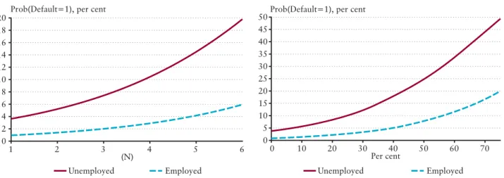
Chart 2 shows the probability response curves of unemployment as a function of the number of dependants, while Chart 3 depicts the ‘unemployment effect’ as a function of the share of debt servicing cost. The marginal effect of unemployment ranges from 2 when the number of dependants is 1, to about 13 percentage points when it approaches 6, which shows that the probability a household will default after the job loss of the main wage earner is far greater for those where the number of dependants is high. Similarly, if we analyse the unemployment effect as a function of the share of debt servicing cost, the marginal effect ranges from 2.7 to 29 percentage points, which indicates that the probability of default after the job loss of the main wage earner is far greater among overindebted households.

Charts 4 and 5 portray the probability response curves of the 5th income quintile dummy. The marginal effect of income is also increasing monotonically with the number of dependants and the share of debt servicing cost. The marginal effects as a function of the number of dependants and the share of debt servicing cost range from 1 to 6.3 and from 1 to 19 percentage points respectively.

Chart 2

Probability response curves of unemployment as a function of the number of dependants (Network 2)

0 2 4 6 8 10 12 14 16 18 20

1 2 3 4 5 6

Prob(Default=1), per cent

Unemployed Employed

(N)

Chart 3

Probability response curves of unemployment as a function of the income share of monthly debt servicing cost

Per cent

Unemployed Employed

0 5 10 15 20 25 30 35 40 45 50

0 10 20 30 40 50 60 70

Prob(Default=1), per cent

25The first logit model (Logit 1) is used for calculating the probability response curves.

3.2. DISTRIBUTION OF ESTIMATED PROBABILITIES AND DEBT AT RISK

The above described analysis showed the influence of different factors on the default probability. In this section we look at default probabilities and debt at risk by grouping households along various single dimensions, taking account of their different attributes and not allowing for unobserved individual effects.²⁶Table C in Appendix 2 shows the mean default probabilities and debt at risk calculated from the above described models, by the households’ region of residence, disposable income, the qualification of the household’s head, taking account of the actual circumstances of those in each group.

Regarding the region of residence,²⁷the mean PDs and the standard deviation of the probability of default are higher among households in less developed parts of the country (North-Eastern Hungary, Northern and Southern Plain). Debt at risk is also the highest in these regions. Depending on the methods used for calculating these risk measures the average PD ranges between 2 and 7.4 per cent, while debt at risk ranges between 3.5 and 22 per cent. The results are not surprising, as these areas are characterised by the lowest net average wage income, which is approximately 85 per cent of the county average, and the highest unemployment and lowest employment rates – 11 and 44 per cent respectively.²⁸As a consequence, the share of debt servicing costs is on average higher, which prevents the accumulation of any reserves and makes these households more sensitive to shocks.

Analysing risks by the qualification of the household’s head, the results suggest that the average PDs are the highest among those whose head has a low qualification (mean PDs range between 1.8 and 6.7 per cent, debt at risk ranges between 6.2 and 10.3 per cent). It is true in general that qualification determines both the permanent income and the labour market possibilities. Low skilled persons are more exposed to adverse movements in the economy, as their work can be easily substituted. In times of economic downturn firms usually lay off their low skilled workers and keep their high skilled ones.

Therefore, low skilled workers’ income might be more exposed to the cyclical fluctuations of the economy. As a result, high income variance might contribute to higher variance in the probability of default within this category. This assumption might be supported by the fact that the standard deviation of the probability of default is the highest among them.

RESULTS

Chart 4

Probability response curves of income as a function of the number of dependants

0 10 20 30 40 50 60 70 80

1 2 3 4 5 6

Prob(Default=1), per cent

Income is not in the 5th quintile Income is in the 5th quintile

(N)

Chart 5

Probability response curves of income as a function of the income share of monthly debt servicing cost

Per cent

Income is not in the 5th quintile Income is in the 5th quintile 0

5 10 15 20 25

0 10 20 30 40 50 60 70

Prob(Default=1), per cent

26Analysing the distribution by multiple dimensions is of no relevance, due to small sample bias.

27Central Transdanubium includes the following counties: Fejér, Komárom-Esztergom, Veszprém; Western Transdanubium includes the following counties: Gyõr- Moson-Sopron, Vas, Zala; Southern Transdanubium includes the following counties: Baranya, Somogy, Tolna; Northeastern Hungary includes the following counties:

Borsod-Abaúj-Zemplén, Heves, Nógrád; Northern Plain includes the following counties: Hajdú-Bihar, Szabolcs-Szatmár-Bereg, Jász-Nagykun-Szolnok; Southern Plain includes the following counties: Bács-Kiskun, Békés, Csongrád; Central Hungary includes the following: Pest county and Budapest.

28Hungary 2006, http://portal.ksh.hu/pls/ksh/docs/hun/xftp/idoszaki/mo/mo2006.pdf, available only in Hungarian.

Analysing risks by income, both the average PDs and debt at risk are the highest among those households whose income is in the 1^stquintile. The average PDs range between 6.2 and 8.6 per cent, while debt at risk is between 10 and 24.2 per cent. The differences in these measures among other income quintiles are not substantial. It has to be mentioned that the effect of income is not necessarily separable from the above analysed factors, as mainly these determine which part of the income distribution the household is located in. Therefore, income is more or less a condensate of information about household’s riskiness stemming from their given sociodemographic features.

In summary, debt payment problems are most likely to occur among households which possess the following attributes: the region of residence is in North-Eastern Hungary, Northern or Southern Plain, the main wage earner has a low qualification and the household disposable income is in the 1st income quintile.

In order to get an overall picture about risk concentration within the group of indebted households we employ the index of concentration of debt at risk – May and Tudela (2005). The index is the ratio of debt at risk and the average probability of default. As the index varies, either because of the probability of default, the value of the debt outstanding, or the combination of these, it may promptly reflect the evolution of risks related to retail lending. If the index value exceeds one it indicates that debt is concentrated among risky households, while values less than or equal to one imply that the risk concentration is not substantial.²⁹

The values of the concentration index are 1.37 and 1.36 in the case of the logit and the network models, while 3.07 by using the non-parametric based framework with original income data, and 2.59 by taking into account the income distortion. The results suggest that, regardless of the methods used for calculating the concentration index, a substantial part of the loan portfolio is owed by potentially risky households, which is unfavourable from a financial stability point of view. Risks are somewhat mitigated by the fact that a substantial part of risky debt is comprised of mortgage loans, which are able to provide considerable security for banks in the case of default.

3.3. THE STRESS TESTING EXERCISE

Stress tests are tools for analysing the shock-absorbing capacity of the banking system in relation to adverse macroeconomic events. With stress tests we can judge whether the banking system acts as a ‘stabiliser’ in the economy, i.e. it is able to absorb shocks and mitigate the negative consequences of business cycle fluctuations or more serious adverse economic events. The key aspects of stress testing are to identify the sources of risks and the channels through which they are transmitted, and to measure their effects on the financial system.

From households’ credit risk point of view two main sources of risks can be considered which have a relatively large significance: declining employment, and fluctuating exchange and interest rates.³⁰ The main consequence of the first is declining disposable income, while the impact of the second on household credit risk develops through the rising cost of debt servicing (the foreign currency finance of Hungarian households, for instance, makes their balance sheet position sensitive to exchange rate and foreign interest rate fluctuations, as they do not have natural hedge).

Regarding the risk transmission channels, three can be detected through which the banking activity is principally affected: the credit risk, the income generation risk and funding risk channels. Funding risk might arise through the credit risk channel as a result of the worsening profitability related to household lending, which might lower market confidence and raise the cost of external finance. Banks are faced with income generation risk when the operational environment becomes unfavourable, which reduces banks’ capacity to generate income (especially net interest and fee income, a substantial proportion of which is related to household lending). Finally, increasing write-offs reflects the deterioration in households’ payment ability.

29For a better understanding of this concept we present a similar example as May and Tudela (2005). Suppose that there are two households A and B. Household A has a debt of 1,000,000 HUF and B has a debt of 500,000 HUF. Suppose that each household has an equal default probability (10 per cent). Then the total debt at risk is 0.1*1,000,000+0.1*500,000=150,000 HUF, that is 10 per cent of the total debt outstanding and the mean PD is 10 per cent. Suppose instead that household A has a 15 per cent probability of having payment problems, while household B has a PD of 5 per cent. In this case the debt at risk is 0.15*1,000,000+0.05*500,000 = 175,000 HUF and the share of risky debt is 11.6 per cent, which is higher than in the previous case. The mean probability of default is still 10 per cent. The index of concentration of debt at risk in the former case (i.e. PDs were equal) is 1 while in the latter case (i.e. PDs differ) it is equal to 1.16 since the household with the larger amount of debt is now more risky.

30Probabilities were not assigned to the occurrence of the various scenarios. This is the task of future research.