MEASURING BANK EFFICIENCY AND MARKET POWER IN THE HOUSEHOLD AND CORPORATE CREDIT MARKETS CONSIDERING CREDIT RISKS*

(1)

MEASURING BANK EFFICIENCY AND MARKET POWER IN THE HOUSEHOLD AND CORPORATE CREDIT MARKETS CONSIDERING CREDIT RISKS*

Zsuzsanna HOSSZÚ – Bálint DANCSIK

(Received: 18 July 2017; revision received: 27 October 2017;

accepted: 3 December 2017)

The aim of this paper is to estimate the effi ciency of Hungarian banks with several models and to calculate the Lerner index for both the household and the corporate credit market. We apply stochastic frontier analysis (SFA) and data envelopment analysis (DEA) models to estimate the effi ciency and calculate profi t and cost effi ciency with and without taking credit losses into consideration. In terms of cost effi ciency, banks are nearly homogeneous and improved their effi ciency after the crisis. Banks, however, are extremely heterogeneous in terms of profi t effi ciency. During the crisis, a gradual improvement could be observed across the sector after the initial downturn.

Since the operating conditions of the household and the corporate credit markets are different, we estimated the intensity of competition separately for both the markets. While the Lerner index showed strong market power in the household credit market, the corporate credit market was characterised by intense competition. Regarding effi ciency, various models often resulted in different conclusions, especially in the case of cost effi ciency. Therefore we recommend that the regulatory decision-making process should always consider the results of several models. Moreover, the Lerner indices demonstrate that it might be important to use disaggregated models when modelling the features of credit markets.

Keywords: bank effi ciency, frontier analysis, Lerner index, credit markets, credit risks, Hungary JEL classifi cation indices: D24, D40, G21, L11

* We are grateful to Tamás Briglevics and Ádám Reiff for their valuable comments and sugges- tions.

Zsuzsanna Hosszú, corresponding author. Senior Economist at Magyar Nemzeti Bank (MNB, the central bank of Hungary), PhD student at Corvinus University of Budapest.

E-mail: hosszuzs@mnb.hu.

Bálint Dancsik, Senior Economist at Magyar Nemzeti Bank (MNB, the central bank of Hungary).

E-mail: dancsikb@mnb.hu.

(2)

1. INTRODUCTION AND LITERATURE REVIEW

The efficiency of the banking sector and the indicators of competition in the credit markets deserve special attention in countries where the financial sources of corporations are provided foremost by the banking sector. A more efficient banking sector and more intense competition yield lower funding costs for the real economy and greater financial deepening and hence, they strengthen potential output growth. However, excessive credit market competition may give rise to higher willingness to take risks, which weakens financial stability and increases the probability of systemic financial crises. From a regulatory point of view, therefore, changes in the level of these indicators may carry important information.

The most usual way to measure the efficiency of banks is by calculating simple ratios like the cost-to-asset ratio (operating expenses divided by the balance sheet total) or the cost-to-income ratio (operating expenses divided by some aggregate income category). While these ratios have the advantage of easy calculation, this alleviates comparison between many market participants (even on an interna- tional level) and the comparison itself can be highly distorted if the business profile of institutions is markedly different. That is one of the main reasons why it can be useful to evaluate bank efficiency not only with simple indicators based on the balance sheet and the profit and loss statement, but through model estimations as well.

Bank efficiency is measured by two types of models: data envelopment analysis (DEA) and stochastic frontier analysis (SFA). Both the models’ aim is to estimate the efficiency of institutions compared to a frontier market participant inside a given population. This means that both DEA and SFA models tackle efficiency in a relative sense, and the estimation results cannot tell us anything about the population’s (e.g. banking sector in a given country) efficiency in absolute terms.

There is no consensus in the literature on which type of models is more appropriate. The DEA models are nonparametric estimations and they were first applied in the article of Charnes et al. (1978). In DEA models, the efficient frontier is the result of a sequence of linear programming exercises and the model identi- fies any deviation from it as inefficiency. The advantage of this approach is that there is no need to make assumptions on the form of the cost function. The use of the second model was first proposed by two articles in parallel with each other:

Aigner et al. (1977), and Meeusen – Van den Broeck (1977). The SFA models are based on econometric estimation where deviation from the efficient frontier is decomposed into a random error and an inefficiency term. Thus, the advantage of these models is that inefficiency is not calculated as a residual, and random ef-

(3)

fects may also deter banks from the efficient frontier. However, the disadvantage of SFA models is that preliminary assumptions must be made on the form of the cost function and the distribution of the error terms, which might lead to mis- specification and biased estimators.

Since both the model types have limitations and advantages, both are often used. Although the literature on bank efficiency estimation is extremely diverse, relatively few articles compare the results of the various estimates. The first article in this regard is the study by Ferrier – Lovell (1990), which estimates the cost efficiency of US banks by using both DEA and SFA methods. They found that although the two techniques yield very similar results regarding the inefficiencies on average, their conclusions about the efficiency ranking of individual banks are different. Eisenbeis et al. (1997) also used US data to compare these two techniques; however, their results are not consistent with the previous article.

The authors found that efficiency levels were different but the ranking of banks was very similar under the two methods. Similarly, Bauer et al. (1998) compared the efficiency estimates on the US banks derived from a DEA model and other 3 parametric models (including SFA model). They concluded that the parametric methods tended to yield higher average cost efficiencies than the DEA model.

While correlation between the rankings of individual models was low and the different approaches identified the best and the worst banks differently. Moreover, each technique proved to be stable over time, but the DEA model slightly outper- formed the parametric estimates. However, the standard financial efficiency indicators (such as the ratio of operating costs to total assets) were more correlated with the estimates of parametric methods.

Huang – Wang (2002) and subsequently Dong et al. (2014) were the first authors to compare the parametric and the nonparametric methods on Asian data.

Using Taiwanese data, the former study found that the two methodologies yield similar average efficiency estimates, yet they resulted in different efficiency rankings of banks. The latter article relied on Chinese banking sector data and found significant differences between the parametric and the nonparametric estimates.

Although results pertaining to the European banking sector are incoherent, the conclusions of more recent articles are very similar to those estimated on the US and Asian data. Drake – Weyman-Jones (1996) estimated cost efficiency among the UK institutions by using DEA and SFA approaches, while Resti (1997) did the same in relation to data on the Italian banking sector. These studies found no significant differences between the results yielded by the two techniques neither in terms of level nor in terms of ranking. Weill (2004) examined efficiency on a sample of Western European banks with both the parametric and the nonparametric methods and found that the average efficiency scores estimated by different models were similar, but the rankings across banks were different. The article

(4)

also examined the relationship between cost efficiency, size and specialisation, and the results yielded by various methods showed differences once again. Casu et al. (2004) examined the degree and the cause of improvement in productivity by means of the parametric and the nonparametric models also on a sample of Western European banks. Although their various estimates led to the same results at sector-level, the models attributed productivity improvement to different factors. Delis et al. (2009) made comparisons between the cost and the profit efficiencies estimated by DEA and SFA models based on a panel dataset of Greek banks. Their results suggested greater correlations between the results of cost and profit efficiency methods than between the results of DEA and SFA models.

To the best of our knowledge, no comparisons have been made between the results of different models in relation to the Eastern European countries, and even the profit and cost efficiency measurement for Greece was compared only by Delis et al. (2009). The lower number of banks and the faster technological changes driven by the convergence process may render efficiency estimates more difficult and uncertain, which provides an even greater reason for the use of several models and the comparison of their results.

In regard to the bank efficiency, the 2008 financial crisis also raised a number of important questions. Firstly, is there a relationship between the efficiency of the banking system and the intensity of financial crises? Secondly, did the events of 2008 exert any impact on the efficiency of banks? Regarding the first question, Diallo (2017) found that more efficient banking sectors were hit less seriously by the global crisis. The author used the DEA method to measure the efficiency of the banking sector. Based on data derived from the South-East European countries, Nurboja – Kosak (2017) concluded that the crisis provided an incentive for banks to enhance their cost efficiency (calculated by an SFA model). One purpose of this study is to examine the second question using Hungarian data; namely, how did the banking sector efficiency evolve and was there any material shift in efficiency at the sector-level as a result of the crisis. According to our results, the cost efficiency undoubtedly but moderately improved in the post-crisis years.

As regards the profit efficiency, however, various estimates did not yield such straightforward results: the models pointed to stagnation or a downturn in the first few years of the crisis. Moreover, although the profit efficiency improved in the period of recovery (from 2013), it is not clear whether this efficiency returned to or exceeded the pre-crisis levels.

In terms of the cost efficiency, the outbreak of the 2008 crisis is important also because of the rise in credit losses and the expansion of non-performing loans. As the crisis unfolded, banks’ non-performing portfolios and credit losses surged both in the emerging and the developing European economies, but the increase showed significant differences between individual banks, in terms of

(5)

banks’ diverging risk appetite. In order to factor in this phenomenon, we added credit losses to the costs typically used in the literature. Then, we compared the results of those models where the differences in risk acceptance were taken into consideration with those where they were ignored.

In this study, we estimated the cost and the profit efficiency on Hungarian data both with DEA and SFA models and compared the results based on the criteria proposed by Bauer et al. (1998). According to our estimates, there are relevant differences between the estimates produced by the two approaches, especially in the case of cost efficiency. The profit efficiency estimates performed better than the cost efficiency estimates even in terms of stability and correlation with clas- sical profitability indicators. Disregarding credit risks may imply the loss of important information; however, it may improve the stability of the estimate. Based on the example of the Hungarian banking sector, this study calls attention to three important considerations: (1) the results derived from DEA and SFA methods may often lead to different conclusions, which underpins the importance of rely- ing on as many methodologies as possible in efficiency estimates; (2) the size of the credit risks may warrant their inclusion in the efficiency estimates; and (3) owing to the heterogeneity of banks’ loan portfolios, the main credit segments (at least the household and the corporate segments) should be included separately in the model.

Previous studies regarding the Hungarian banking sector’s cost efficiency did not offer a straightforward conclusion. Depending on the methodology, the estimated period and the sample, the estimates classify the Hungarian banks into mixed categories: some studies place them among the leaders of the CEE countries (Koutsomanoli-Filippaki et al. 2009), others (Fries – Taci 2005; Niţoia – Spulbar 2015) in the middle of the ranking, yet others (Molnár – Holló 2011) among the least efficient ones. In terms of bank competition, literature found diverging trends in the household and the corporate credit segments. Previous studies focused primarily on frictions in the household credit market,¹ while in- tensive competition was reported in the corporate credit market.

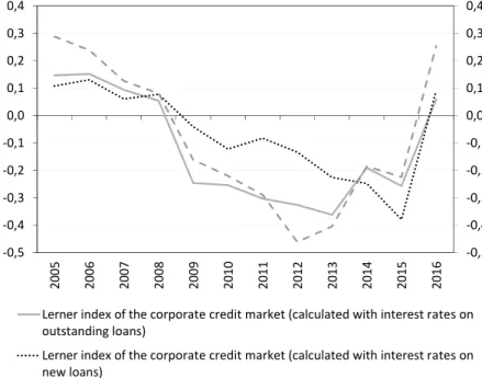
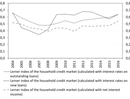
We calculated Lerner indices by using the SFA type cost functions. In our estimates household and corporate loans were treated as separate outputs based on the assumption that the two credit markets behave differently.² This expecta- tion was confirmed by the estimated Lerner indices. The intensity of competition proved to be different in the two segments both in terms of level and dynamics.

1 See, for example, Móré – Nagy (2003, 2004), Molnár et al. (2007) and Kézdi – Csorba (2012).

Aczél et al. (2016) also emphasise the role of market power as a determinant of housing loan spreads.

2 The reason behind this is explained in detail in Section 2.

(6)

We constructed the indices by using two different methods in consideration of credit risks. This did not cause a significant variation between the estimates. Fi- nally, we also compared the Lerner indices calculated on the basis of the average lending rate on new disbursements and on the outstanding portfolio. We found that the former tends to respond to market developments more quickly than the latter and therefore shows more significant variations.

We structured our study as follows: Section 2 presents the specification of models, explains why we chose the assumptions concerned and provides a brief overview of the data used for our estimations. In Section 3 we discuss our find- ings in detail, and finally in the last section we conclude.

2. METHODOLOGY AND DATA

Numerous possible model specifications are available both for the DEA and the SFA type models, which are different from each other in terms of certain sub- assumptions. We had two goals in mind when we selected the specification of the models: on the one hand, we wanted to ensure that our assumptions are as consistent with the known properties of the banking sector as possible, and on the other hand, we wanted our assumptions for DEA and SFA models to be the same wherever possible, for the sake of comparability.

In calculation of banks’ efficiency, we modelled the production process in each approach to examine how much output can be produced from certain inputs at the given input prices and how much did it cost or how much profit could be achieved.

In these calculations, human resources and fixed assets are generally considered as inputs, and the loan portfolio, interest-bearing assets and/or all other assets are included as outputs. The models typically do not include more than three inputs or outputs; their number can be increased only with certain constraints.³

As mentioned above, we examined profit and cost efficiencies separately. The necessity of profit efficiency measurements comes from the heterogeneity of the model outputs, which can be attributed to numerous reasons for it to be different from cost efficiency. For example, the loan portfolio (which is typically included as a homogeneous product in the cost efficiency estimates) can be regarded as heterogeneous in several regards. This heterogeneity can be caused by potential maturity mismatches within the portfolios among other things. If a bank grants a higher percentage of shorter-term loans, it will face higher costs owing to the

3 In the case of SFA models, this is probably because high number of explanatory variables in the estimation would significantly increase uncertainty. As regards to DEA models, too many business models would be considered efficient as a result.

(7)

faster velocity of the loans, and the bank will end up having a worse cost efficiency score than other banks. However, the lending rates on short-term loans might be higher; therefore, this bank will have higher revenues and may even perform better than other market participants in profit efficiency. Similarly, if a loan portfolio is considered homogeneous, it gives rise to the problem that the performing and the non-performing portions of the portfolio will be treated by the models uniformly. This can alter the results significantly, especially in times of financial crises when the increase in the non-performing portfolio may considerably be different at individual institutions. This is because the earning potential of non- performing portfolios is lower compared to the rest of the loans, whereas the operating expenses associated with such portfolios is typically higher. The diverse cost implications of individual credit products also counteract homogeneity: for example, in household lending the disbursement of a mortgage loan and an unsecured consumer loan can imply substantially different costs, which is enforced by the bank in its pricing; i.e. in the profit. Therefore, if banks specialise in different segments and the number of outputs defined in the cost function is too low, then both DEA and SFA methods may identify inefficiencies even in cases where the higher or the lower level of costs simply results from different composition of assets. However, there are also arguments for the use of cost efficiency: profit efficiency is more sensitive to the cyclicality of the real economy as cyclical events affect the profit through risks and interest revenues as well. Consequently, the improvement in productivity could be better captured by cost efficiency.

We selected three products for our outputs: our models include household loans, corporate loans and other interest-bearing assets. From a theoretical perspective, the two credit markets may differ in costs, entry barriers and consumer behaviour. In the household credit market the same portfolio requires a broader branch network and a higher staff number on average compared to the corporate credit market, where loan sizes are larger. Building up the required branch network also means a higher entry barrier in the market of household loans. Moreo- ver, households tend to be less rational or less informed than corporate clients, and also they usually obtain loans of a considerably smaller amount.⁴ Another difference between the two segments is the difference of information asymmetry prevailing in these two markets: while banks can analyse the financial statements

4 In view of this, it was by no accident that the foreign banks appearing in the CEE countries after the collapse of the Soviet Union often specialised in corporate lending; in fact, in many cases they followed the multinational corporations operating in the home countries of the re- gion (Havrylchyk 2005). The case was similar in Hungary: with respect to household lending, foreign banks lagged behind the OTP Bank, a bank deeply rooted in the household segment for many years, which is also indicative of the former institutions’ competitive disadvantage and the higher costs of entry, typical in this segment.

(8)

of companies allowing them to obtain information both before and after the trans- action, this is only partly true for the household credit market, especially in the later years of the loan term.⁵

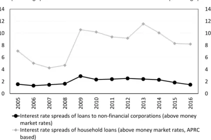
Moreover, owing to the high share of loan products with unilaterally adjust- able interest rates, banks had a pricing advantage in the Hungarian household credit market relative to the corporate credit market that was dominated by float- ing rate schemes. Indeed, before 2012 the Hungarian legislative environment was lenient about the modification of lending terms during the term of the loan, and banks could conceive legal solutions that allowed them to unilaterally raise the interest rate on a loan at basically any time until it is matured. Most institutions took advantage of this opportunity, and after the outbreak of the crisis this led to an increase in the interest rates of already disbursed household loans by 150–200 basis points on average. This scheme was far less common in the case of corporate loans, partly because of the better bargaining position of the sector and partly because of shorter maturities. Subsequently, we also test the marked differences between the two loan segments through the Lerner index. The heterogeneity of the loan portfolio in efficiency estimates is also justified by the differences mentioned above.

The banking sector is often modelled as a financial intermediary or a money creator. In the first case, financial liabilities appear among the inputs, whereas de- posits are included among the outputs in the latter assumption. In consideration of the Hungarian banking sector’s heavy reliance on foreign financing and because we already included three outputs with the decomposition of the loan portfolio, we opted for the financial intermediary approach.

In both the model types, certain constraints can be applied with respect to the returns to scale (if there is a constraint, it generally assumes constant returns to scale). Since we examined the banking sector of an emerging country that has suffered a series of structural breaks; and as severe market frictions should be expected due to asset market’s protracted adjustment resulting from the long maturities, we assumed variable returns to scale.⁶

These models usually do not factor in the credit losses, even though they represent regular and significant expenditures for banks and their volume is not negligi- ble compared to the operating expenses. At the same time, business (accounting) decisions and cyclical events may strongly influence the loan loss provisioning.

5 Although at the conclusion of the contract even the household customers need to verify their financial and wealth situation, it is far more difficult for banks to monitor changes in the financial situation of a retail debtor in the later years of the term than in the case of corporate loans where regular accounting statements are readily available.

6 We also test this assumption and will discuss the results in more detail in the sections of specific models.

(9)

Since our sample also included a crisis period when credit losses were extremely high, we found it particularly important to explicitly include these expenses in our models. This procedure is not common in the literature and it is not clear how these items should be incorporated into the models. Our solution is described in the sections of specific models.

Time dimension is another important factor to consider when estimating DEA and SFA models. The relationship between inputs, prices and outputs is not only shaped by efficiency, which is in the centre of our interest, but also by macroeco- nomic, regulatory and technological changes. These factors can be (somewhat) controlled for by dividing the sample to smaller subsamples with a shorter time- frame, or by explicitly controlling for the time dimension by including time variables into the estimation. However, these solutions can be highly constrained if the database available is not long or wide enough (i.e. short time horizon, too few institutions) to include more variables in the parametric estimation.

One can easily see that while model-based efficiency estimations are much more sophisticated compared to the calculation of simple accounting-based ratios, the interpretation of such models can be tricky considering all the assumptions and the broad variety of possible modelling decisions. The higher number of possible model choices also indicates that there is some uncertainty around the concept of efficiency when estimating it with either the parametric or the nonparametric models.

2.1. SFA models

The total cost or total profit function can be written as:

( , , , , ),

it it it it it it

TC C Y W Z u e (1)

where TC_it is the total cost or total profit of bank i in period t. Y_itis the vector of outputs, W_it is the vector of input prices and Z_it is the vector of additional control variables in the case of bank i in period t. u_it expresses the banks’ deviation from the efficient frontier, while e_it is the random error. We estimate the equation in logarithmic form as follows:



^, ^,



it it it it it it

lnTC c Y W Z lnu lne (2)

where lnu_it captures the deviation from the effi cient frontier and therefore, its value is always non-negative in cost functions and non-positive in profi t functions, and lne_it is a normally distributed random noise.

(10)

We need at least two more assumptions for estimating the equation: the exact form of the cost function (c) and the distribution of the inefficiency term. In addition, it is also possible to include specific variables identifying u_it(e.g. Greene 2005), but we did not opt for this solution for two reasons. Firstly, we did not want to impose further constraints and secondly, we wished to ensure the comparability of our results with DEA models. As regards to the cost function, we assumed the most widely used functional form in the literature: the translog function. We assumed that the distribution of u_it was exponential. Accordingly, our estimated equation is the following:

0

1 2 1

2

it j jt k kt jl jt lt

j k j l

km kt mt jk jt kt s st it it

k m j k s

lnTC lnY lnW lnY lnY

lnW lnW lnY lnW lnZ lnu lne

α β γ δ

θ μ

   

     

  

  

(3)

where TC_it denotes total cost or total profit of bank i at time t, Y_jt denotes total output of product j at time t, W_ktdenotes input prices of input k at time t, and Z_st denotes additional control variables at time t.

We derived the coefficients and the error terms from maximum likelihood estimation, in accordance with Wang’s (2002) estimation method. Some estimates included the household and the corporate loan loss provisioning as input prices, however, certain cross products linked to loan loss provisioning were neglected from these models. Since two new input variables would have considerably increased the number of estimated parameters, we took into consideration only the cross products of loan-loss provisioning and loan amounts. Because of the limitations regarding the number of parameters, we could not include the time variables into the model.

2.2. DEA models

DEA models describe banks’ cost minimisation or profit maximisation problem in the form of a linear programming exercise. The original model that assumes constant returns to scale for a specific bank can be written as follows:

*0

* 0 0

, 1

0 1

1,2, , min

0,

i

m

i i

x n

j rj r

j

r s

w x

y y

λ



 

 



(4)

(11)

* 0 1

1,2, , 1,2, 0,

0 ,,

n

j ij i

j

i m

x

n x

j λ

λ







 

 



where n, s and m denote the number of banks, outputs and inputs, respectively, while x^*_i0 is the cost-minimising vector at constant input (w_i0) prices and output levels (y^*_r0). Accordingly, the optimal vector is a linear combination of the inputs of those banks that produce at least as many outputs as the given bank without using more inputs. The efficiency of the evaluated bank can be calculated by comparing its actual cost level to the optimal cost level that is the efficiency of bank j = w_ijx^*_ij/ w_ijx_ij. Thus the deviation from the efficiency frontier is equal to

1- _{ij ij}^*/ _{ij ij}

i i

w x w x

 

. In the case of efficient banks, this value is zero. If a bank produced negative profit in a year, we determine profit inefficiency to be equal to 1.⁷ Due to the definition of the model, the sample will always include a perfectly efficient bank.

As mentioned before, instead of constant returns to scale we assumed variable returns to scale. As a result, an additional condition was added to the model in relation to weights:



ⁿ_j_₁λ_j 1. Equation (4) is based on the assumption that the input prices are uniformly given for each bank. This assumption is questionable from the perspective of funding costs; indeed, the foreign-owned banks or those in a better solvency position can generally access the less expensive funds. There- fore, we adjusted the model in line with Tone’s (2002) proposition: each bank fac- es unique input prices, and the input prices were included in the inequality conditions applied to inputs. Moreover, we incorporated the loan loss provisioning of the loan portfolios and the control variables applied in SFA models into our DEA models as well, as quasi-fixed costs. Similar to the model proposed by Gulati and Kumar (2016), an inequality condition must hold for quasi-fixed costs in the same way as for the other costs. The quasi-fixed costs, however, do not appear in the objective function and they are not decision variables. Thus, the model used for the estimation of cost efficiency took the following form (where z denotes the quasi-fixed costs, while other denotations are the same as in equation 4):

7 While this method is in line with the literature, it is worth noting that this method may lead to loss of information if the majority of banks are in fact producing a loss. Bos – Koetter (2011) offer an alternative specification to alleviate this problem, where they change negative profits to be 1, and add an indicator variable that takes the absolute value of the losses, while for profitable banks the indicator variable is zero in logs.

(12)

*0

* 0 0

, 1

0 1

* 0 0 1

0 1

1

min

0, 1,2, ,

0,

1,2, ,

1

0 1 , ,, ,2

i

m

i i

x n

j rj r

j n

j ij ij i i

j n

j kj k

j n

j j

j

w x

y y

w x w x

z

r s

i m

k

j

z p

n

λ

λ λ



 



 

 







 



(5) Again, efficiency is received as the rate of optimal and actual costs. Profit efficiency is calculated on the basis of the same logic. All its assumptions are identical with those applied in the cost efficiency exercise, except for one: the output inequality constraint is replaced by a constraint pertaining to revenues.

The revenues of bank j are denoted by R_j:

* *

0 0

* *

0 0 0

, , 1

* 0 0 1

0 1

* 0 1

1

*

0 0

*

0 0

max

0,

0

1,2, ,

0

,

1,2 ,

1 ,

0, , ,

i

m

i i

x R

n

j ij ij i i

j n

j kj k

j n

j j

j n

j j

i i

j

R

i m

k p

i m

j w x

w x w x

z z

R R

x x

R R

n

λ





 



 



 







 





(6) Finally, another assumption must be introduced for the estimation about whether the efficient frontier should be considered constant or variable over time. If we opt

(13)

for the latter, then the n parameter will indeed mean the number of banks and optimisations must be run separately for each individual period. If, however, we assume that technology remained constant throughout the review period, then the n index will be the product of the number of banks and the number of periods, in which case optimisations are performed all at once. While this assumption does not change the number of linear programming exercises that should be run, it changes the number of bank observations to be considered during one exercise. The latter option is sup- ported by the argument that in the case of a small number of banks, the use of too many conditions would lead to a result where too many banks are extremely efficient. However, it supports the use of the former option that DEA models do not take account of the random shocks sustained by banks and consequently, in this approach technology may easily change every year. Finally, we decided to take the middle road: we divided our sample into four parts, the operating environment of the banking system was roughly the same within each sub-sample. The first period lasts from 2001 to 2004, when the Hungarian banking sector was characterised by balanced growth and forint-denominated loans. 2005–2008 was a period of excessive credit expansion and indebtedness in foreign currencies. 2009–2012 were crisis years producing the greatest downturn, while 2013–2016 mark the period of recovery.

Accordingly, if we do not apply any constraint on the amount of λ_j-s, we assume constant returns to scale, while if we introduce the condition of 0



ⁿ_j_₁λ_j1 , then the returns to scale will be non-increasing. If the sum of λ_j-s equals 1, the technology has variable returns to scale. We also ran simulations with the lenient assumptions and checked for equality between the optimal results in different cases. Since the solutions were different for both lenient constraints, we decided to opt for the assumption of variable returns to scale and used this condition for SFA models as well.

2.3. Data

We used a balanced panel database that included the data of 12 Hungarian banks for the period between 2001 and 2016. The database includes banks which (1) have operated since 2001 in a continuous manner and (2) are operating on a market-based principle (i.e. we didn’t include those banks in the database, which have special responsibilities stemming from the state, for example the Hungarian De- velopment Bank and the EXIM Bank).⁸ We examined the data at an annual fre-

8 The database contains the following banks / banking groups: Budapest Bank, Cib Bank, Erste Bank, FHB Bank, Fundamenta, K&H Bank, KDB Bank, MKB Bank, OTP Bank, Raiffeisen Bank, UniCredit Bank, Volksbank / Sberbank. These institutions cover approximately 84 per cent of the Hungarian banking system on the basis of total asset.

(14)

quency, obtaining a total of 192 observations in the sample. With respect to the data, we relied on the statistics compiled by the Magyar Nemzeti Bank (MNB) (including balance sheet, profit and loss statements and interest rate statistics). The number of observations in our database can be considered as less than ideal, however expanding it would only be feasible partially and not without sacrifices.⁹

As mentioned before, we defined three outputs for the cost efficiency estimates: retail loans, corporate loans and other interest-bearing assets. The vast majority of retail loans consist of the loans granted to the household segment (mortgage loans and unsecured consumer loans). Corporate loans include loans granted to large corporations and SMEs as well. The majority of other interest- bearing assets represent government bonds and instruments issued by the central bank, while loans disbursed to other sectors (such as local governments) make up the smaller part of these assets. The inputs and their prices presented in the model are consistent with those commonly used in literature. As inputs, we included interest-bearing liabilities (their price is the rate of interest expenses and interest- bearing liabilities), personnel costs (their price is the ratio of personnel costs to balance sheet total) and material expenditures, including amortisation (their price is the ratio of expenditures and the bank’s total assets). The loan losses input includes the impact of loan loss provisions and also profit effect of portfolios sold at a price under their net value.¹⁰ In the case of cost efficiency estimates, the dependent variable is the sum of operating expenses and interest expenses, while in the case of profit efficiency models, our dependent variable is the sum of net interest income and net fee and commission incomes less operating expenses. In the estimates where loan losses were considered, we also added the impact of loan loss provisioning to the dependent variable.

We used three price variables for estimating the Lerner index. In addition to the interest income / interest-bearing asset ratio typically used in the literature, we also had the data needed to calculate the index with the average interest rate (or, in the case of the household segment, the APR) on new loan contracts and with the average interest rate of the portfolio weighted by loans outstanding.

9 Expanding the time dimension of the database would be possible by using data with a quar- terly frequency, however considering the peculiar characteristics of banks’ operations (i.e.

loan loss provisions set aside typically at the end of the year, or money-market transactions af- fecting banks’ income more than one quarter within a year with an opposite sign) would bring substantial noise into the data within a year. The cross-section dimension of the data could be expanded with more institutions, however, these banks are special institutions operating on niche markets, which would make them outliers in our efficiency estimations.

10 Due to space limitations we could not include the detailed description of the database and the regression tables in this paper, however, it is available in Hungarian in the MNB Occasional Pa- per version of this study (Dancsik – Hosszú 2017), or in English if requested from the authors.

(15)

The use of the latter two price variables is not common in literature, mainly because these statistics are published by central banks only at the sector-level.

The same is true for breaking down the former indicators by loan segment:

household and corporate interest income/interest rates can be rarely obtained from public data sources.

3. RESULTS

Upon the estimation of SFA models, few control variables from the pool of possible control variables were eventually excluded from the estimates. The Lambda statistics – the ratio of the standard deviation of the two error terms – is an important sign of a bad specification. Therefore, we included only those control variables where the Lambda statistics took a value close enough to 1. In the case of profit functions the model includes only the size of capital buffers, whereas in the case of cost functions it includes the size of capital buffers, the percentage of liquid assets and the number of branches. In DEA models the variables included as quasi-fixed costs are the same as the control variables used for the corresponding SFA estimates.

3.1. Comparison of the model results

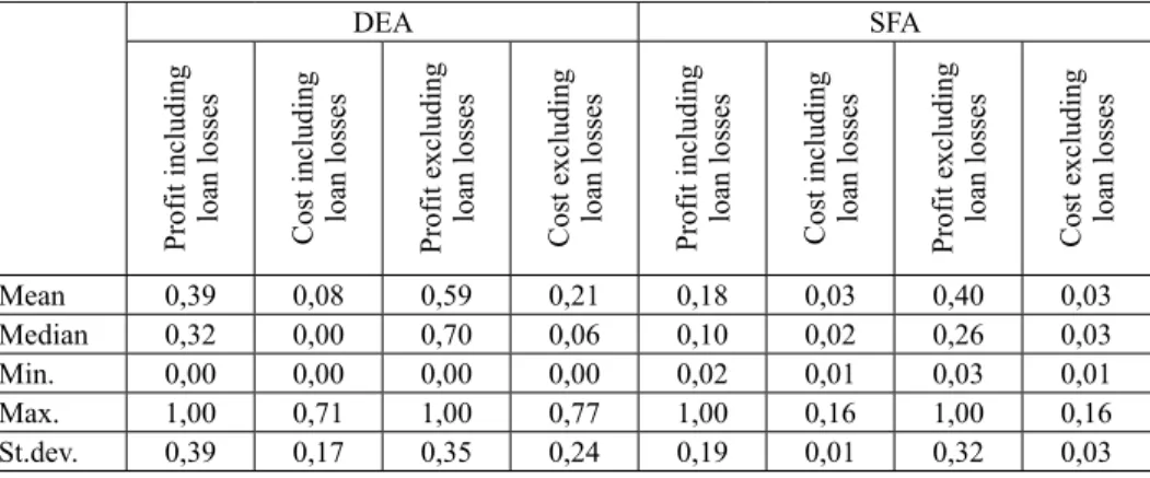
In line with the procedure of Bauer et al. (1998) and Dong et al. (2014), we analyse the relationship between the results of the models in 5 steps and evaluate the estimates. In the first step, we compare the descriptive statistics of inefficiency terms (Table 1).

Both the model families identified high cost efficiency and much lower profit efficiency based on boththe mean and the median. Interestingly, even the median is zero for the cost efficiency calculated in DEA model which takes the loan losses into account. It means that at least half of the banking sector was quali- fied as perfectly efficient by the model.¹¹ Usually, the distribution of inefficiencies was slightly or more strongly left-sloped (except for the profit function of

11 We would like to highlight here one more time that efficiency is always a relative concept in these models. We should keep in mind that when the model results indicate high average efficiency, it is only interpretable within the population of the Hungarian banks in the database.

Based on these models we cannot state anything about the absolute efficiency of the Hungar- ian banking sector as a whole (e.g. compared to other countries’ banking sector), i.e. it is possible that the Hungarian frontier itself is highly inefficient when compared to banks in other countries.

(16)

DEA model that disregards loan losses), which suggests that the distributions are more likely to show the outliers pointing to the worse performance. As regards the minimums, SFA models do not consider either bank as perfectly efficient, whereas DEA models identified perfectly efficient banks in all cases. In the case of the observed maximum inefficiencies, the profit functions indicate the most inefficient banks. However, regarding the cost functions, the range of inefficiencies is far greater in DEA models. Owing to the higher maximum values, the standard deviations are higher in DEA models both in terms of profit and cost efficiency.

Therefore, we may conclude that DEA models are more likely to show extreme efficiency values and that the banking sector is more homogeneous in terms of cost efficiency than in terms of profit efficiency.

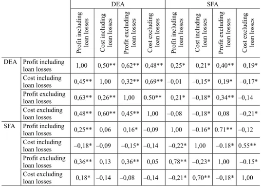
The second aspect of the assessment is the comparison between correlations and rank correlations (Table 2). Our results are consistent with the part of the literature that points to a weak correlation between the two estimation procedures.

Out of the 16–16 possible correlations and rank correlations we received positive values only in 2 and 3 cases, respectively, that were significant at 1 per cent level. Within the model family, the DEA results were moderately correlated (at all traditional significance levels), while the cost and profit efficiency estimates demonstrated a significant difference in the case of SFA models. Nevertheless, the strongest correlation was found within SFA models; the smallest differences occurred in estimates that included or excluded loan losses. Consequently, DEA models proved to be more robust, overall, for the specific model specification, but minor differences only slightly alter the results of SFA models. Moreover, the profit efficiency results showed a significant positive correlation even between the two model families (DEA and SFA), while this was not the case with cost ef-

Table 1. Descriptive statistics of inefficiencies (total sample)

DEA SFA

Profit including loan losses Cost including loan losses Profit excluding loan losses Cost excluding loan losses Profit including loan losses Cost including loan losses Profit excluding loan losses Cost excluding loan losses

Mean 0,39 0,08 0,59 0,21 0,18 0,03 0,40 0,03

Median 0,32 0,00 0,70 0,06 0,10 0,02 0,26 0,03

Min. 0,00 0,00 0,00 0,00 0,02 0,01 0,03 0,01

Max. 1,00 0,71 1,00 0,77 1,00 0,16 1,00 0,16

St.dev. 0,39 0,17 0,35 0,24 0,19 0,01 0,32 0,03

Source: Own calculations.

(17)

ficiency. Therefore, profit efficiency is more robust for the estimation procedure than cost efficiency.

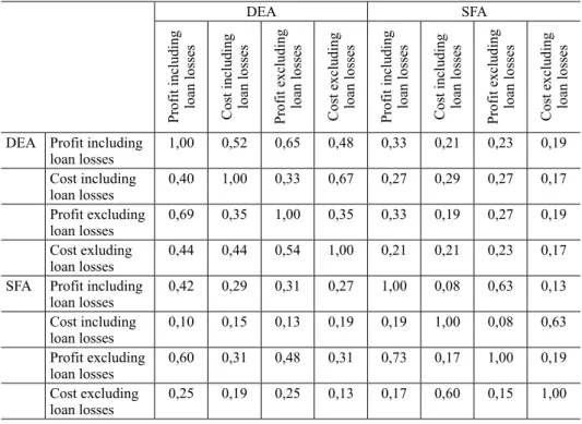
We can conclude similar statements to those derived from the correlations by comparing the set of banks considered to be the best and the worst by different methods (Table 3). The two approaches generate different results based on the percentage of the same banks classified into the top or the bottom quartiles and once again, the results of DEA models are closer to each other. It was also recon- firmed that SFA models examining profit efficiency are more likely to arrive at similar results as those received by DEA models than the models estimating cost efficiency, irrespective of whether the DEA estimate was intended to gauge profit or cost efficiency.

We examined the stability of the estimated inefficiencies by autocorrelations (Table 4). None of the model estimates can be considered strongly autocorre- lated, and even medium autocorrelations occur only in first-order cases. When comparing the parametric and the nonparametric methods, neither method can

Table 2. Correlation and Spearman correlation of inefficiencies

DEA SFA

Profit including loan losses Cost including loan losses Profit excluding loan losses Cost excluding loan losses Profit including loan losses Cost including loan losses Profit excluding loan losses Cost excluding loan losses DEA Profit including

loan losses 1,00 0,50** 0,62** 0,48** 0,25* –0,21* 0,40** –0,19*

Cost including

loan losses 0,45** 1,00 0,32** 0,69** –0,01 –0,15* 0,19* –0,17*

Profit excluding

loan losses 0,63** 0,26** 1,00 0.50** 0,21* –0,18* 0,34** –0,14 Cost excluding

loan losses 0,48** 0,60** 0,45** 1,00 –0,08 –0,18* 0,08 –0,21*

SFA Profit including

loan losses 0,25** 0,06 0,16* –0,09 1,00 –0.16* 0.71** –0,12 Cost including

loan losses –0,18* –0,09 –0,15* –0,14 –0,22* 1,00 –0.18* 0.55**

Profit excluding

loan losses 0,36** 0,13 0,36** 0,05 0,78** –0,23* 1,00 –0.15*

Cost excluding

loan losses 0,18* –0,14 –0,08 –0,14 –0,21* 0,70** –0,18* 1,00 Note: Correlations that proved to be significant at 5% and at 1% significance levels are denoted by * and **, respectively. The upper triangle contains the correlations, while the lower triangle shows rank correlations.

Source: Own calculations.

(18)

Table 3. Classification of best and worst banks, (%)

DEA SFA

DEA Profit including

loan losses 1,00 0,52 0,65 0,48 0,33 0,21 0,23 0,19

Cost including

loan losses 0,40 1,00 0,33 0,67 0,27 0,29 0,27 0,17

Profit excluding

loan losses 0,69 0,35 1,00 0,35 0,33 0,19 0,27 0,19

Cost exluding

loan losses 0,44 0,44 0,54 1,00 0,21 0,21 0,23 0,17

SFA Profit including

loan losses 0,42 0,29 0,31 0,27 1,00 0,08 0,63 0,13

Cost including

loan losses 0,10 0,15 0,13 0,19 0,19 1,00 0,08 0,63

Profit excluding

loan losses 0,60 0,31 0,48 0,31 0,73 0,17 1,00 0,19

Cost excluding

loan losses 0,25 0,19 0,25 0,13 0,17 0,60 0,15 1,00

Note: The values in the upper triangle show the percentage at which banks belonging to the worst quartile cor- responded to each other. The lower triangle indicates the same value for the best quartile.

Table 4. Autocorrelations

DEA SFA

1 0,32 0,12 0,49 0,37 0,49 0,18 0,47 0,30

2 0,25 –0,03 0,37 0,18 0,19 –0,15 0,16 0,05

3 0,20 0,01 0,18 0,09 –0,03 –0,22 0,11 0,09

4 0,12 0,14 0,08 0,22 –0,14 –0,09 0,01 –0,01

(19)

be deemed more stable than the other in general; stability depends on the conditions and on the order of the autocorrelation. By contrast, profit efficiencies are more strongly autocorrelated than cost efficiencies, except for the fourth-order autocorrelation. Similarly, the models estimated without the loan losses generally appear to be more stable than the calculations that take the loan losses into account. Indeed, we observed negative autocorrelations in the case of the latter.

Presumably, this is because the exact value of the loan loss provisioning can be strongly influenced by accounting considerations; moreover, the prudent banks tend to recognise higher loan loss provisioning for large expected losses, which are partly reversed after the actual losses have been realised.

Since the stability of inefficiency measures is weak, we calculated the autocorrelations of inefficiencies for each individual bank to examine the heterogeneity among banks (Table 5). In the case of the model estimated with the loan losses, autocorrelations were weak for almost all banks independently from the chosen estimation method. However, the other inefficiency indicators are characterized by high heterogeneity at individual level in almost all cases; the calculated autocorrelations spread from weak negative to very high values. These results suggest that large, bank specific shocks are common in our sample.

Table 5. First order autocorrelation of inefficiency measures for each bank Profit

including loan

losses

Cost including loan

losses

Profit excluding loan

losses

Cost excluding loan

losses

Profit including loan

losses

Cost including loan

losses

Profit excluding loan

losses

Cost excluding loan

losses

1 0,91 0,45 0,78 0,61 0,75 0,18 0,81 0,19

2 0,21 –0,11 0,12 0,45 0,59 0,09 0,28 0,16

3 0,47 –0,09 0,71 0,45 0,59 0,29 0,72 0,62

4 0,86 –0,11 0,51 0,05 0,41 0,14 0,41 0,09

5 0,40 0,32 0,66 0,63 0,76 0,07 0,88 0,18

6 0,00 –0,07 0,54 –0,07 0,20 –0,01 0,17 0,28

7 –0,30 0,15 –0,20 0,10 0,40 0,38 0,13 0,29

8 0,92 0,85 0,94 0,79 0,23 0,04 –0,04 0,37

9 –0,42 0,15 –0,04 0,54 0,82 0,40 0,72 0,61

10 0,55 0,15 0,72 0,20 0,16 0,37 0,77 0,38

11 0,31 –0,07 0,76 0,14 0,47 0,08 0,47 0,13

12 –0,12 –0,15 0,35 0,57 0,54 0,12 0,32 0,28

Note: Autocorrelations higher than 0.6 (strong autocorrelations) are signed with gray colour.

(20)

Finally, we compared the estimated inefficiency measures with the profitability and efficiency indicators derived from financial indicators (Table 6). We use four financial time series: return on average assets (ROAA), return on average equity (ROAE), ratio of total costs to total assets (TC/TA) and efficiency ratio (ER) (ratio of non-interest expenses and revenues). Since a higher value means a more profitable bank in the first two cases and a less efficient bank in the last two cases, we expect the estimated value to negatively correlate with the first two and positively correlate with the last two indicators. Our models yielded mixed results based on these criteria as well: in the case of ROAA and ROAE, the profit inefficiency estimates produce the expected results with the appropriate sign and significance level, and the SFA estimates perform better than the DEA estimates.

This should not be surprising, given that profitability as profit efficiency estimates both consider expenditures and revenues alike. By contrast, it is clearly the DEA estimates that perform better in the case of the TC/TA indicator, regard- less of whether they measure cost or profit efficiency. The results yielded by the SFA estimates do not match even in terms of sign. Our models demonstrate the worst performance in relation to the efficiency ratio; it is only in the case of cost efficiency ratio measured by DEA model without loan losses that a positive correlation can be observed at 5 per cent significance level.

The significant differences between the model results highlight the importance of the decisions and the assumptions lying behind the estimations. The SFA models are estimated on a longer time horizon, and are more flexible to the effect of shocks because of the random error term included in the model, while the DEA models are more prone to identify individual shocks as a change in efficiency.

Table 6. Comparison between the estimated inefficiencies and financial profitability and efficiency indicators

DEA SFA

ROAA –0,14 0,14 –0,2* 0,23** –0,43** –0,09 –0,35** 0,11

ROAE –0,18* 0,07 –0,24** 0,18* –0,45** –0,04 –0,37** 0,12

TC/TA 0,18* 0,39** 0,35** 0,33** –0,17* –0,04 –0,05 –0,07

ER –0,18* 0,07 –0,24** 0,18* –0,45** –0,04 –0,37** 0,12 Note: Correlations that proved to be significant at 5 per cent and at 1 per cent significance levels are denoted by * and by **, respectively.

(21)

The difference between the two types of models is most spectacular in the year of 2012 characterised by more than one unique event, e.g. the early repayment scheme (and parallelly paying back foreign funds), the deepening euro crisis, and tensions in the FX swap market. At the same time, the low correlation with traditional efficiency ratios shows that these models grasp different aspects of efficiency, compared to the aspect offered by simple accounting-based ratios. All in all, we can conclude, that in order to develop a comprehensive evaluation of efficiency, it is essential to analyse it from more than one perspective.

3.2. Effect of the crisis on effi ciency

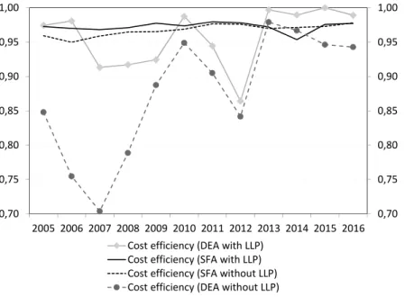
Our results indicate that in terms of cost efficiency, the Hungarian banking sector is relatively homogeneous, even weaker banks are close to the efficient frontier. This high relative effectiveness is confirmed by the results of SFA model throughout the entire sample, but only for the last few years of the sample by DEA model.

The DEA (and to a smaller extent the SFA) estimates indicate that the Hungarian banks have improved their cost efficiency since 2005. The substantial part of this improvement took place after the outbreak of the crisis in parallel with a substantial cost adjustment (Figure 1). This relatively fast adjustment, however, was not followed by an additional significant improvement, in which the erosion of banks’ loan portfolios played an important part (between 2009 and 2015, the loan portfolios declined continuously both in the household and the corporate segments). Conse- quently, the environment was not supporting for an improvement in cost efficiency.

The results of efficiency estimates are volatile. The DEA estimates point to a relevant decline in efficiency in 2012. This may reflect a government measure, the early repayment scheme of mortgage loans at a preferential rate, as a result of which a substantial part of a highly profitable portfolio was removed from banks’

balance sheet in two quarters.¹² Banks could make cost adjustments only with some lag owing to the rapid time profile of the measures. This led to a temporary decline in efficiency. The efficiency estimates including loan losses showed a slight negative swing once again in 2014, reflecting exceptionally high write- downs by two large banks. The DEA results differ from each other greater than

12 Under the scheme, mortgage debtors indebted in foreign currency had an option to repay their loans at a far more favourable, fixed exchange rate instead of the prevailing market rates. As a result of the programme, the household loan portfolio shrank by HUF 1,041 billion (HFSA 2012), which accounted for almost 13 per cent of the loans outstanding before the launch of the programme.

(22)

the results of SFA models. This could be owing to the fact that in case of the SFA estimations, one part of the shocks is identified as random error, while in DEA models, these shocks figure as inefficiencies.

As regards profit efficiency, the standard deviation among banks is far greater compared to the cost efficiency estimate and it is far more difficult to identify a clear trend throughout the 11-year period we examine. This shows that a substantial part of the inefficiency may be attributable to the revenue side of the profit and loss statement. The marked differences between the cost efficiency and the profit efficiency estimations confirm that there are aspects of inefficiency which do not stem from the relationship between inputs and outputs (in terms of stocks), but depend much more on the ability of banks to gather income from its existing assets. This finding is not surprising given the high level of non-performing loans characterizing the Hungarian banking system in crisis years.

Looking more closely to the estimation, the pre-crisis period was featured by a gradual deterioration (Figure 2), which was also reflected in the gradual decline in the ROAA and ROAE profitability indicators of the banking sector.

The deteriorating efficiency can be attributed to the saturation of markets and to

0,70 0,75 0,80 0,85 0,90 0,95 1,00

2005 2006 2007 2008 2009 2010 2011 2012 2013 2014 2015 2016 Costefficiency(DEAwithLLP)

Costefficiency(SFAwithLLP) Costefficiency(SFAwithoutLLP) Costefficiency(DEAwithoutLLP)

Figure 1. Cost efficiency estimate of Hungarian banks based on SFA and DEA cost functions Note: The above values express individual banks’ cost efficiency weighted by balance sheet total, showing how close banks’ operational efficiency is to the efficient frontier on average. Higher values indicate higher efficiency levels.

Source: Own calculation.