Disaggregated Household Incomes in Hungary Based on the Comparative Analysis of the Reweighted Household Surveys of 2010 and 2015*
Mihály Szoboszlai
In the period 2010–2015, the Hungarian employment rate recorded an outstanding increase even by European standards. During this period, the Hungarian Central Statistical Office recorded a 9 per cent increase in the number of employees, coupled with a 15.5 per cent rise in net real wages. This study presents the evolution of these indicators broken down by income groups. In addition to number of employees and labour incomes, changes in the total compensation of pension and social benefit recipients are also discussed in the study. Calculations are based on the 2010 and 2015 data waves of the household budget statistics. One disadvantage of using these data, however, is that they are distorted along the income distribution due to the phenomenon that high earners are typically represented by a low number of observations. The study presents a two-step recalibration procedure with previously unused cohort formation that addresses the aforementioned coverage deficiency with adjustment to external data sources. The material well-being of different household income groups can be tracked in the database produced by the applied method, and the macroeconomic indicators can be supplemented by pieces of distribution information. According to the results defined as the difference between the two years’ data under review, the employment growth in the interim period was determined by the employment of the two lower income quintiles. In the assessment of social benefits, with the limited information available, the chosen tool does not provide a comprehensive view of the changes in these income categories; therefore, the quantified differences between the reweighted sample years’ data should be considered with caution. Broken down by income group, real wage indices exhibited considerable fluctuations.
Journal of Economic Literature (JEL) codes: D31, D33, J31
Keywords: Income, income distribution, wage distribution, well-being, household statistics, reweighting
* The papers in this issue contain the views of the authors which are not necessarily the same as the official views of the Magyar Nemzeti Bank.
Mihály Szoboszlai is an Economic Analyst at the Magyar Nemzeti Bank. E-mail: szoboszlaim@mnb.hu This article presents the author’s views and does not necessarily reflect the official opinion of the Magyar Nemzeti Bank. The author owes a debt of gratitude to Balázs Kóczián and Balázs Sisak for their thorough reading of the manuscript and for valuable recommendations regarding the presentation of the study’s results.
Special thanks go to Izabella Kuncz for her helpful comments and clarifications, Ákos Pogány for his remarks on the income of foreign employees and Dóra Kerényi-Bräutigam for conscientiously monitoring the initial
1. Introduction
The current state of well-being has constantly been the focus of attention of political decision-making and social science. This is mostly monitored by measuring households’ current incomes and consumption expenditures. Regularly published statistics denote national economy totals, based upon which one can make statements with respect to material well-being on the basis of averages. At the same time, family revenues and expenditures by both individuals and specific household segments may emerge erratically in an economy. A prerequisite for exploring the distribution characteristics of these is the availability of a micro database that provides reliable, sufficiently detailed information for such an in-depth analysis.
In Hungary, the Household Budget and Living Conditions Survey (HBLS) gathers detailed information on the consumption expenditures, living conditions and collected incomes of respondent households. The expenditure side of the HBLS is structured in accordance with the classification of individual consumption by purpose (COICOP-nomenclature1), which offers the most comprehensive statistics as far as the granularity of product breakdown is concerned and is applied uniformly across the European Union Member States. Similarly, revenue data are structured in numerous income categories; however, in terms of coverage, the data collection is typically deficient around the tails of the income distribution. In order to answer differentiated questions about the living standards of various social groups, this deficiency needs to be remedied. Consistency between the waves of the micro database that serves as the primary data source is a crucial prerequisite for the accuracy of quantitative analyses. In this study, I use a peculiarly applied tool to resolve the methodological problem and then, with the information of the pre- prepared database, changes in the welfare of the individual income quintiles are examined by comparing these cross-sectional surveys of 2010 and 2015.
Besides general interest, there is growing professional demand for the publication of distribution information on welfare (Stiglitz – Sen – Fitoussi 2009). With the availability of such information one can analyse the processes of social/income differentiation. When inequality is increasing in a society to a degree that exceeds the increase in per capita welfare indicators, a large proportion of individuals may find themselves in a weaker financial situation even though welfare is improving (on average). Besides the shift of centre of welfare gravity, monitoring the behavioural responses of groups at the bottom and at the top of the distributions may also provide useful outputs from a social and economic policy perspective.2 The reform ideas of the Fitoussi report gave fresh impetus to the development of information
1 For more details on the methodology of the classification, see: UN (2000).
2 The new macroeconomic forecasting model of the Magyar Nemzeti Bank also places a particular emphasis on the heterogeneity of households, as shown in detail in the working paper by Békési et al. (2016).
systems and inspired innovative thinking about the data while encouraging more prudent data use.
According to the recommendation of the Stiglitz report, the most evident approach to measure material well-being in an alternative manner would be the addition of distribution information to total economy-level statistical data. However, it should be noted at this point that comparing the indicators included in the national accounts with data derived from the survey can be challenging.3 On the one hand, a considerable portion of the earnings captured at the macro level may not actually appear at the level of households (see, for example, imputed rents at market price, or the interest spread between preferential and market rates); on the other hand, the corrections performed to ensure the comprehensiveness of the national accounts (estimates regarding the level of unreported and hidden incomes) may also increases the discrepancies between the two data sources. According to general experience, household surveys offer limited insight into income at the individual level. In addition to the respondent burden, income concealment and respondents’
low willingness to reply to sensitive questions about their well-being, reliable data gathering is hampered by the fact that households are not aware of certain income types on an item-by-item basis. Finally, the comparison also runs into difficulties, as in many cases the published consumption and income indicators do not include breakdowns that can clearly be attributed to actual data aggregated from the survey (e.g. labour incomes from full-time employment, cost reimbursement(s) or the forms of pension received on own right).
2. Data
The primary data source of the analysis is the Household Budget and Living Conditions survey conducted by the Hungarian Central Statistical Office. The HBLS contains about 8,000 to 10,000 private households (15,000–20,000 individuals) representing the total Hungarian population. The database collects product-level data on the value of the goods and services purchased by households and provides detailed information on households’ stock of durable goods. Besides consumption habits, the survey contains questions relating to households’ relative financial situation and indebtedness. Since it takes account of more than 60 – person or household-related – income types annually, it provides an opportunity for a detailed analysis that offers substantial information on the well-being of households both from a consumption and income perspective. The benefit of using the household database as opposed to administrative data sources (e.g. the registry of personal income tax returns, pension register, other official registers) is that it collects information on diary-keeper respondents not only on an individual basis, but also
3 Exploring the differences may be facilitated by the description of the methods and data sources applied in
at the household level: therefore, the types of households in which the persons participating in the survey can be identified.
The analyses were based on the HBLS conducted for 2010 and 2015 (HCSO 2011;
2016); the main difference between the data collections of these two years was the accounting of incomes. In the 2010 data wave, households4 reported on the reviewed income categories in gross amounts, while from 2013 onward they made a statement on their material well-being in net terms. The reason for this accounting difference that in 2013, the HCSO adjusted the budget survey to the methodology of the international living conditions survey (European Union Income and Living Conditions Survey). As a result of the harmonisation, the list of the survey’s income variables and the contents of the variables changed (somewhat), which were standardised during the analysis. Net categories were created from gross income data for 2010 based on own calculation in accordance with the prevailing tax tables and transfer rules.
One of the external (secondary) databases used for the purpose for improving the data quality of the HBLS is the full sample of the anonymous PIT returns for the years 2010 and 2015. Using information from the database, a substantial part of personal incomes has become available at the personal level by sex, age and county (see sub-section 4.2). Data on pension benefits, in turn, have been corrected in accordance with the number of recipients contained in the statistical yearbooks of the Central Administration of National Pension Insurance (in Hungary abbreviated as ONYF) (see sub-section 4.1). Other benefits were not revised during the imputing process as beneficiaries often receive non-pension type transfers with some main sources of income (labour and/or retirement income); therefore, any database correction on this basis would specifically modify, assumedly to an undesired degree and direction, key income items.
3. Methodology
3.1. Approaches in European countries: merging with administrative data This section discusses the statistical-methodological issue of how typical the usage of administrative data is among countries compiling European living standard surveys. The main data source on income, poverty, social exclusion and living conditions in the European Union is the EU-SILC (European Union Statistics on Income and Living Conditions) survey. Most Member States have been increasingly moving towards the use of administrative information for statistical purposes. The obvious benefit of re-using data is the simultaneous reduction of data collection costs and the burden on respondents. In addition, a further advantage of the use
4 For the purposes of the calculations I used the survey with its weights adjusted to the baseline figures of the 2011 census; consequently, in longitudinal section the sample weights of the chosen years are balanced.
of official data is the improvement of the quality of the self-assessment based responses provided in existing surveys, as well as the updating and rationalisation of survey questionnaires. Merging the individuals participating in the survey to a register containing the characteristics in question through a unique identifier is the most direct way of data use. In many cases, the linkage is established by providing the person’s social security or the personal identification numbers or in some countries the combination of name, address, place and date of birth information.
At the European level, the extent of the practical utilisation of administrative data varies across countries and statistical institutions. Differences can be explained not only with legislative obstacles but, as will be shown later, certain cases raise some questions in terms of quality. In the latter case, two aspects should be carefully taken into consideration: timeliness and comparability. Timeliness issues arise because of the fact that the contents of the registers are released by data owners with a significant lag due to the time-consuming nature of the data processing practices that intends to ensure the internal consistency of the registers. In addition, the methodological changeover to the use of administrative data may affect comparability across time and definitions country by country, which should be carefully assessed by the national statistical offices envisaging an increased use of registers.
Countries compiling the EU-SILC survey can be divided into two groups: the groups of “register countries” and “survey countries”. In the register countries, the use of external registers is more broad-based in designing and conducting the survey.
Register countries typically comprise Scandinavian countries and Slovenia (Table 1), where a single unique identifier is used to merge numerous registers. The countries using administrative data sources, however, exhibit differences based on the extent to which they draw upon such data sources. For instance, regarding income types, Denmark, Finland, Iceland, Ireland, the Netherlands, Norway, Slovenia, Sweden and Switzerland collect income data mostly from registers, while other countries can only utilise information on certain income components and/or certain sub- populations. For the most part, SILC countries rely on official data sources to substitute demographic and income variables. Typical registers also comprise data on education, labour market and housing market, but these are used in relatively few countries. Denmark, Slovenia, Iceland and Norway are the four countries where each type of register listed above is used to compile the SILC survey. Recently, the active implementation of income registers has been completed or is in progress in France, Latvia, Switzerland and Ireland, while Austria and Spain are in the implementation/assessment phase (Di Meglio – Montaigne 2013).
Table 1
Use of administrative data in Europe
Administrative data Countries Total (number)
Demographic/household data BGR, BEL, DNK, EST, ESP, FIN, ITA, LVA, LTU, NLD, AUT, SWE, SVN,
IZL, NOR
15
Education data DNK, FIN, SVN, IZL, NOR 5
Labour data BGR, DNK, NLD, SVN, IZL, NOR 6
Housing/dwelling data DNK, AUT, GBR 3
Income data BGR, BEL, CYP, DNK, EST, FIN,
FRA, IRE, ITA, LTU, LVA, MLT, NLD, AUT, SWE, SVN, IZL, NOR, CHE
19
Electricity and water
consumption MLT 1
Not using administrative data CZE, DEU, GRC, HUN, LUX, POL,
POR, SVK 8
Note: The table uses the three-letter country codes (ISO alpha-3).
Source: Di Meglio – Montaigne (2013)
In the “survey countries”, it is the legal environment that most often hinders the use of administrative data sources (Table 2). In the EU-SILC context, legal infrastructures need to allow the linkage of register information to survey data, the dissemination of micro data to Eurostat,5 as well as further dissemination to third parties (i.e.
researchers). A precondition for using registers is the broad, public approval of their use, especially since respondents must be informed of the use of register contents during sample surveys. Confidentiality may be legislated, for example, through data protection laws or laws on the processing of personal data, which have a wider scope than the provisions governing statistics (UN 2007).
5 As a Directorate General of the European Commission, Eurostat provides EU institutions with statistical data and harmonises statistical methodologies across the Members States and EFTA countries, as well as candidate countries. Its databases are available free of charge over the internet.
Table 2
Main reasons reported by countries for not using register data
Reason for not using register data Countries Total (number)
Registers are not available CZE, DEU, POL, SVK 4
Legal issues that
prevent access to these sources DEU, HUN, POL 3
prevent linking of these sources GRC, HUN, LUX, POL,
PRT 5
prevent the dissemination of micro data from these
sources HUN, PRT 2
Quality and methodological issues EST, GRC, LUX, PRT 4
Note: The table displays the three-letter country codes (ISO alpha-3).
Source: Di Meglio – Montaigne (2013)
In addition to legislative constraints, efficient data utilisation during the design or assessment of surveys is hampered by the lack or insufficient quality of registers.
Countries facing qualitative and quantitative problems are Estonia, Greece, Luxembourg and Portugal. The most typical drawbacks are poor data quality and the substantial amount of missing information. Methodological differences in these countries are caused by the contents of the variables included in the surveys and in the registers and the difference between the observation units and the classification categories. Insufficient coverage also poses a challenge.
3.2. Methods applied in the Hungarian practice
In the second half of the 1990s, several studies were published on the validity of household statistics (Révész 1995; Éltető – Havasi 1998). The accuracy of the survey in terms of social/economic statistics was investigated compared to macroeconomic indicators in a wide range. Subsequently, due to the sampling procedure the survey provided a fairly accurate from a social perspective, but the bias of consumption and income representativeness remained an inherent feature of the survey. Numerous Hungarian studies have attempted to bridge the latter discrepancies.
Hosszú (2011) simultaneously uses the income and consumption data of the household survey in one (economic) framework. Although the author performed calculations on raw data without any correction, she notes that the quantile measures used to indicate income disparities (the ratio of the income of the ninetieth and tenth percentiles is [p90/p10]) were unreliable in the lowest and uppermost deciles due to the deficiencies of the survey, and for this reason, it is more prudent to compare the second and the ninth deciles in the longitudinal comparison, instead of the differences between the lowest and the uppermost income deciles.
Benczúr et. al (2011) and Benczúr – Kátay – Kiss (2012) attempt to ensure the representativity of the survey with respect to labour income by percentile matching.
The essence of the method is to map, percentile by percentile, the wage incomes in the household budget survey to the individual tax returns data and then to adjust the wage incomes of the survey for the average wage of each percentile from PIT data. This approach produces similar results regarding the representativeness of the HBLS with respect to earnings as the multiple matching of survey information and individual tax return data. This procedure was also used on the dataset presented by Benedek – Kiss (2011).
Cserháti – Keresztély (2010) propose two kinds of imputation methods for achieving consistency between the data of household survey and macroeconomic statistics.
In the case of compensation of employees, cost reimbursements and earnings from self-employment and agricultural production, using personal tax return data the authors creating cohorts according to three variables (income deciles, region and age), which are matched with the corresponding cohorts of the HBLS.
The principle is similar as in the case with Benczúr – Kátay – Kiss (2012), with the difference that the applied cohort formation in their case covers more dimensions.
Lastly, the authors adjust the number of employees and average income data of the corresponding groups in the HBLS to the group averages of the tax returns.
The second imputation method proposed by the co-authors is reweighting (also referred to as recalibration). Using modified values included in the HBLS, they alter the original survey weights according to property income applying an iterative algorithm for a multivariable optimisation problem – for more detail on this method, see the studies by Darroch – Ratcliff (1972) and Molnár (2005). The advantage of this method is that HBLS data, which become available with a lag of one and half years, can be updated and forecasted with the method of reweighting. Because of timeliness, results included with the unchanged weighting may cause bias. As noted by Cserháti and Keresztély, the method can be combined with any other cohort formation criteria. The next section presents a data imputation based purely on such reweighting. The section also addresses the dilemmas arising during the reweighting procedure.
4. Reweighting the Household Budget Survey
The reweighting algorithm presented later in the study serves a dual purpose. On the one hand, it is desirable to have a detailed database that is representative from the view of income, in which consumption expenditures and incomes earned by households can be examined in conjunction. If only incomes are adjusted to the whole economy aggregates calculated from administrative data sources, consumption-income ratios will have a one-sided bias in the survey. At the same time, it is generally observed regarding household living condition surveys that
respondents tend to report more accurately on their expenditures and liabilities than on their incomes and material well-being. Being aware of these facts, the applied data cleansing methods are assumption-dependent. The other (parallel) objective of reweighting is the creation of a dataset that can be better utilised from the income side for labour market simulations and impact studies.
I reweighted the household budget survey in accordance with the number of persons in each cohort derived from external data sources. It is also possible to perform the reweighting according to total amount of compensation, but this approach has two disadvantages: on the one hand, the application of the selected method does not ensure the non-negativity of the new weights, and on the other hand, the number of persons in the groups created may differ significantly from what can be observed. In the case of recalibration according to the number of persons, the cohort averages will be close to the average values of the secondary data sources if the created groups split the database into sufficiently detailed subsamples. It is a disadvantage, however, that in the primary database few individuals can represent group(s) with a large sample size.
The design of the new weighting system is sequential. First, I reweight the number of recipients included in the HBLS with the group sizes created according to sex and age in the electronic annexes of the Central Administration of National Pension Insurance (ONYF 2010; 2015) and then adjust the taxpayers participating in the survey to the group sizes of individual personal tax returns. Selecting timeliness is required because of the phenomenon of post-retirement employment, which is handled by the adjusted weights applied to the age groups of 60–65 and above.
One precondition for reproducing and disaggregating the macrodynamics is that the aggregates derived from the personal income tax return data be close to the published statistical data, or the sufficiently accurate representation of most inter-period changes by the sub-population included in the survey. In such cases, the temporal change computed from the difference between the two cross- sectional surveys is nearly equivalent to the change computed from the official macroeconomic indicators.
It is important to underline that reweighting is performed at the level of individuals;
household-level weights are produced by averaging the weights. Meanwhile, it should also be noted that the reweighting algorithm affects only certain groups, which strongly depends on the groups that are formulated. For example, if the number of 35–45 year-old men earning (purely) a gross wage income of HUF 3–5 million per year in one of the reference years is identical in the survey and in the PIT database, they will be considered representative for the purposes of the analysis, and the original weights applied in the survey will remain unchanged. Obviously, the
weights will remain unchanged in the case of households composed of individuals who earn non-taxable income or non-pension type benefits.
4.1. Reweighting of recipients of pension on own right
In the case of recipients of pension benefits, the most promising external data source is the complete payment database of the National Directorate for Pension Disbursement (in Hungary: NYUFIG). However, information was unavailable for the years required for the analysis. The statistical yearbooks of the ONYF publish two- dimensional contingency tables only, and do not show at the individual level the number of different benefits paid for recipients. Cserháti – Keresztély (2010) simply assume that the marginal distributions of the frequency tables are independent, therefore the authors receive the joint distribution by the desired attributes as the product of the marginal distributions. They determine the joint distribution from the distribution of age groups of beneficiaries calculated from year of birth and of the average amounts of pensions by region. The control numbers of the reweighting presented in this study are from the tables of the number6 of recipients in each sex and age group. Geographic matching is outside of the scope of this analysis. The list of variables in the HBLS typically includes benefits received on the recipient’s own right (old-age pensions, disability annuities, survivors’ or orphans’ benefits).
For this reason, from the annexes of the yearbooks I used the number of persons receiving full benefits7 of the recipients entitled to pension on their own right.
4.2. Reweighting according to tax return data
The use of anonymous tax return data raises the need of harmonising the income variables of the two data sources. One disadvantage of using tax return data is that individual taxpayer income categories cannot be compared with incomes reported in the HBLS due to differences in definitions. The category of “other wage incomes”
include several social insurance and social benefits (e.g. pregnancy and infant care benefit, child care benefit, jobseeker’s benefit and health care allowances) that are treated as wage incomes in personal taxation but are unidentifiable. The identification of “other income from other than self-employment” in the HBLS (e.g.
remuneration received by senior officers or elected office-holders, income paid for personal contribution) causes similar difficulties and inconsistencies, as it is unclear which income types are used by the respondents to report such items. The income types used for personal PIT data are therefore restricted to wage income, cost reimbursements, entrepreneur’s withdrawals, representative taxpayers and income from agricultural production.
6 Older age groups were defined uniformly both in PIT return data and in the statistics of the yearbooks (55–59, 60–64, 65–74 and 75+) in order to address the aforementioned phenomenon of post-retirement employment.
7 In the case of pensions, instead of main benefits, I consider the column data of full benefits as the point of reference as recipients often are not aware of the supplementary benefits received; therefore, they are expected to report and include in their diaries the pension received in cash via postal delivery.
Compared to the group formation mentioned above, the classification described here is different both in terms of criteria and income collocation. To create a dataset that is best suited for the data requirement of a labour market microsimulation, I reweighted the household survey according to sex, age group, income group and number of taxable incomes using the information of personal tax returns.
I formulated income groups in the datasets by income brackets rather than by commonly used quantiles (Benczúr et al. 2011; Benczúr – Kátay – Kiss 2012; Cserháti – Keresztély 2010).8, 9 The advantage of this classification is that there is no need to reweight the entire household survey population according to income, as the right tail of the frequency distribution of tax return data is heavier than that of the income distribution deduced from the HBLS. Apart from these reasons, it is also important to consider the number of different income sources individuals might earn, because – due to the lack of this information – the reweighting would be biased since we would allocate such incomes to individual respondents that they did not actually receive.
4.3. Limitations of reweighting
The drawback of the reweighting exercise is that the baseline figures of the original, uncontrolled weights become biased. It should be stressed, however, that reweighting according to more criteria would be practically unfeasible, due to the sample size because the individuals participating in the survey are classified into more than 250 groups (around 8,000 households and 20,000 persons). The system of design weights, in line with the census data, is representative in terms of sex, age group, region, education, economic activity and number of children (Éltető – Mihályffy 2002; Molnár 2005). In the case of pensions, regional and demographic distributions are altered with a relatively minor error (10,000–20,000 recipients), due to the reweighting, and the number of persons comprising the retired population remains nearly unchanged after the imputation.
In the case of employees’ earnings, the degree of the bias is substantial for two reasons. Firstly, this is because there are more taxpayers (weighted) in the household survey in each wave than the number of taxpayers registered in PIT return data. As a result, the application of the new weights reduces the number of taxpayers at the
8 Annual income limits applied: HUF 0, 500,000, 1 million, 3 million, 5 million, 10 million, 15 million and 90 million. Personal tax return data reveal that there are few taxpayers with an annual income of more than HUF 90 million, and since we did not observe any in the household sample and since their behavioural responses may significantly differ from the responses given by other individuals, I did not modify the weights of the survey for this information.
9 The implicit assumption of the resulting income classification is that the under-reporting of the survey’s
level of the whole economy,10 and this result also affects the number of households in each income group. Nevertheless, the reweighting does not change the average number of households in the whole economy significantly. Another type of bias is caused by the phenomenon that not all (taxable) income categories are observed in the HBLS (for example, no individuals with more than three sources of taxable income are included in the survey, and thus these individuals are also left out of the aggregation). Furthermore, in the survey the initial weight remains unchanged for those individuals who did not have to submit a mandatory tax return in the given calendar year (mostly small agricultural producers, those who earn tax-free income or income(s) not subject to tax, as well as, wage earners with income from simplified employment below the tax return limit amount).11
5. Results
5.1. Income structure in individual quintiles (2015)
In the analysis, households were classified into groups based on their equivalent incomes (adjusted for household size). One reason for using (equivalent) incomes calculated on the basis of the equivalence scale is that some household-level expenditures increase in line with the number of household members (e.g. food consumption, clothing), whereas no such linearity can be observed in the case of other expenditures (e.g. housing). On the other hand, not only personal incomes determine personal well-being, which is affected by the income situation of the rest of the household members as they together constitute a single consumption unit.
Instead of applying the traditional OECD equivalence scales (OECD 1982; Hagenaars et al. 1994), I used the square root of the number of household members – a practice that has become increasingly widespread in recent years.12
Income types comprising the bulk of the total income of the total population (labour incomes, pensions, social assistance and allowances) exhibit large differences in individual income quintiles (Figure 1). In order to illustrate the marked differences observed at the tails of the income distribution, the income quintiles are decomposed into deciles in Figure 1. The income deciles clearly indicate that the income structure in the lowest and top two deciles differs significantly from that
10 The 2015 survey identified nearly 1,150,000 more taxpayers than the external tax return data. In practical terms, it is a methodological issue as to whether the reweighting of the individuals in the lowest income categories (earning the minimum wage or less) is reasonable as the number of wage earners considerably exceeds the number of persons registered in the tax return data. During the procedure, no dedicated correction was applied in adjustment of PIT data. However, the technique is sufficiently flexible to accommodate such considerations. For example, Benczúr – Kátay – Kiss (2012: 9) do not apply any wage correction steps in the three lowest income deciles.
11 For the mathematical background of the reweighting and for the impact of the applied methodology on the weighting system and on income distribution, see sub-sections F.1 and F.2 of the Annex.
12 For more detail on the scale thus defined, see, for example OECD (2011); OECD (2008), or the studies by Cseres-Gergely et al. (2016: 909) on the HBLS dataset. The impact of the application of the scale is discussed in the study by Éltető – Havasi (2002).
of the deciles representing the middle class (the finer the scale, e.g. it is divided into vigintiles [20 equivalent groups] or percentiles [100 equivalent groups], the greater the inequality between the bottom and the top of the distribution). Among households’ current incomes, income from wealth is typically under-reported in the survey. This category includes profits/returns from property rents and from the holding of financial instruments. Since this information is not available from external micro databases and disaggregated statistical statements, these categories are not reviewed during the analysis even though they represent a sizable source of income within the revenues of Hungarian households.
In 2015, roughly half of the income earned by the lowest income group is labour income13 and social benefits (pensions, social assistance and allowances). The share of pension-type benefits increases up until the third quintile (6th decile), with a decline in the rest of the income categories. This can be primarily attributed to
Figure 1
Income structure in 2015 in households’ equivalent income quintiles/deciles
0 400,000 800,000 1,200,000 1,600,000 2,000,000 2,400,000 2,800,000 3,200,000 3,600,000 4,000,000
0 10 20 30 40 50 60 70 80 90 100
decide1st 2nd decide 3rd
decide 4th decide 5th
decide 6th decide 7th
decide 8th decide 9th
decide 10th decide Employment income
Income from self-employment
Foreign income Cost reimbursement
Social transfers
Family allowances Other income
Pension
Median Income (right-hand scale)
Per cent HUF
Note: Other income includes: income from agricultural production, income from intellectual property, income from service contracts, tips, scholarships, payments from insurance transactions, balance of voluntary funds, interest received, dividend, capital gains, gift/consumption from own production, child support received, tax allowances, in-kind benefits, the total income of children under 16 and other inco- me not identified or reported elsewhere. It is important to emphasise that a negligible number of res- pondents provide information on financial assets in the survey; consequently, this item is not discussed in the sub-sections presenting the results of the analysis.
Source: Calculated from data in the 2015 wave of the HBLS (HCSO 2016)
household size: small-size pensioner households are classified into the middle quintiles (deciles) based on net income per consumption unit. Entrepreneur’s income represents a larger share in the upper income quintiles. Labour income is the most dominant income category among households classified into the fifth quintile (including income from work and/or self-employment and the related cost reimbursement contributions), while non-pension type public transfers practically disappear from the income sources of the uppermost deciles. Typically, incomes from abroad are insufficiently observable in the survey because, on the one hand, these households cannot be reached at the place of domestic residence as they are located abroad at the time of the survey and, on the other hand, in many cases the persons reporting on the gross/net income of household members do not have comprehensive information due to the differences in taxation.
The right-hand axis of Figure 1 presents the scaling of the median equivalent incomes of each quintile. The net disposable income of the lowest quintile is HUF 450,000 (per consumption unit), while households in the top decile earned HUF 3,550,000 per consumption unit in 2015. The median income of the middle quintiles amounted to HUF 1,490,000. Accordingly, incomes are distributed asymmetrically between the lowest quintile and the median earner (p50/p10: 3.05) and between the median earner and the top quintile (p90/p50: 2.53).
5.2. Decomposition of the difference between real incomes (2010–2015) 5.2.1. Perceived inflation – real earned income
In order to obtain the most accurate picture of the well-being of Hungarian households, the earnings of the income quintiles were deflated by the perceived inflation of the quintiles. The perceived inflation14 of individual quintiles is defined as the price change weighted with households’ own consumption structure. The distribution of perceived inflation by quintile exhibits a peculiar duality in 2015:
while the lower income quintiles may have perceived a minor degree of inflation (+0; 0.1%) in the indicator calculated from the representative basket, the topmost income quintiles still perceived a similarly negligible decline in the price level (–0.4;
–0.5%). In a low-inflation environment, the differences in the perceived inflation of individual income groups tend to decrease. Compared to the price levels observed in 2010, perceived inflation ranged between 9.3 and 10 per cent by income quintile in the period under review.15
14 The annual price indices of products and services in the consumption basket are published in the information database of the Hungarian Central Statistical Office. See: http://statinfo.ksh.hu/Statinfo/
haDetails.jsp?query=kshquery&lang=hu.
15 The divergence observed in 2015 can be mainly attributed to the decline in fuel prices. Between 2010 and 2015, cumulated perceived information changed as follows in individual quintiles: 1st quintile: 9.5; 2nd quintile: 10; 3rd quintile: 9.8; 4th quintile: 9.5 and 5th quintile: 9.3 per cent, respectively.
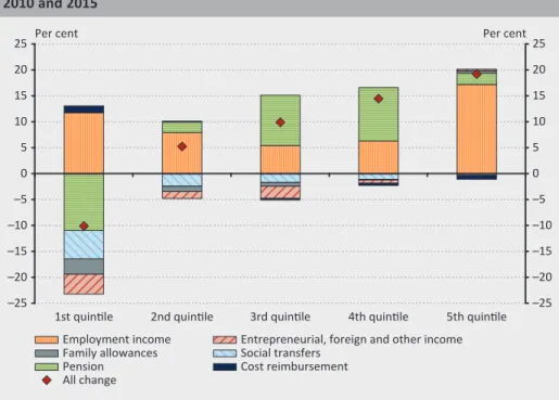
Figure 2 shows a decomposition of the real income differences of individual quintiles into six different categories. As for their low share, entrepreneur’s income, income from abroad and other income constitute one category in the chart. With respect to Figure 2, note that the columns indicate the differences between total compensations; in other words, the chart illustrates the combined effects of the differences between the number of individuals and income levels.
In addition, it should be emphasised that the income flows between the income groups cannot be observed over time since, due to the rotated panel16 nature of the survey, respondents cannot be traced over this time horizon, which renders the interpretation of the results fairly cumbersome. Thus, for example, with respect to the disability pension of the bottom income quintile in 2010, pension income may change because the person in that group receives a lower amount of (rehabilitation) benefit, or he becomes an old-age pensioner during the six years of the examination period, which entitles him to a higher amount of benefit (old-age pension). Similarly, the number of persons in the group may decline if the person in question loses his
16 The term indicates that one third of the respondents is replaced every year; therefore, two thirds of the diary-keeper households are the same from year to year. Another consequence of this rotation is the Figure 2
Decomposition of real income differences into equivalent income quintiles between 2010 and 2015
–25 –20 –15 –10 –5 0 5 10 15 20 25
–25 –20 –15 –10 –5 0 5 10 15 20 25
1st quintile 2nd quintile 3rd quintile 4th quintile 5th quintile Employment income
Pension Social transfers
Family allowances Entrepreneurial, foreign and other income Cost reimbursement
All change
Per cent Per cent
Source: Calculated from HBLS data for 2010 and 2015 (HCSO 2011; 2016)
benefit, or the number of retirees in the quintile may also decrease if the person is classified into a higher income bracket due to a change in his income position and/or household conditions (e.g. he forms a household with a higher-income individual).
Changes in these numbers, therefore, affect average benefit levels. Overall, when comparing the results of equivalent household incomes from cross-sectional data (in 2010 and 2015) it is important to keep in mind that the absolute changes in structure, in flow, and within individual groups can occur simultaneously, and these cannot be separated from one another.
The equivalent household income of the lowest income quintile fell by 10 per cent in 2015 compared to the reference year 2010, while material well-being gradually improved in the rest of the quintiles in each group between 2010 and 2015. The drop in the income of the lowest quintile reflects a peculiar restructuring progress.
The social benefits of this income group were reduced, while the compensation of employees gradually increased. The increment (positive difference) observed in labour incomes was more or less offset by the decline in pension-type benefits, while there was a concurrent decline in social benefits that are considered as a typical source of income in this quintile. From the second income quintile to the fifth quintile, in 2015 both pension benefits and salaries increased in real terms compared to the income situation observed in 2010 (Figure 3). For easier interpretation, it is worth decomposing the differences further in accordance with changes in number17 and wages (Table 3).
Table 3
Decomposition of the cross-sectional differences between real labour incomes in 2010 and 2015 by income quintile
Income groups Number of employees Change in real wages Change in the real wage bill
1st quintile 19% 19% 42%
2nd quintile 18% 9% 28%
3rd quintile 4% 11% 15%
4th quintile –1% 15% 14%
5th quintile 5% 23% 29%
Aggregated change 8.9% 15.3% 25.4%
Note: The values of the table indicate absolute changes; in other words, they do not reflect contributions expressed in proportion to all changes (Cf. Figure 3: in 2010, the labour incomes of the lowest income quintile accounted for 28.6 per cent of the group’s total household income. Thus, the 42 per cent increa- se in total real compensation indicated in the table contributed to the changes affecting households between 2010 and 2015 by 12 per cent (rounded value) on Figure 3.
Source: Calculated from HBLS data for 2010 and 2015 (HCSO 2011; 2016).
17 There were numerous income tax related changes in legislation during the period that had a positive effect on (long-term) employment. The results are discussed in the occasional paper of Szoboszlai et al. (2018).
The comparison of cross-sectional data suggests a double-digit expansion in the number of employees in the period under review. The difference between employment in the lowest two quintiles amounted to almost 20 per cent in the review period, whereas the corresponding value is fairly small in the third and fifth quintiles. Based on the results of the two reweighted samples, the number of employees does not show any difference in the fourth quintile. The employment rates of the lowest quintiles can be attributed to a base effect and to the economic upswing in the period. During the recovery, a large number of employees returned to the domestic labour market in the lowest quintiles, and employment numbers were also boosted by the job protection action plan and the public work programme.
The majority of employees in the middle and upper income group retained their jobs (the changes measured may have been also influenced by flows between the groups). Changes in net real wages show a significant degree of volatility in between the two examined years. Net wages were significantly influenced by the comprehensive personal income tax reform implemented during the period, but this paper is not intended to analyse the distribution and behavioural effects of the relevant tax law changes. The real wages of the lowest quintile are up 19 percentage points in the 2015 survey compared to the reference year, which is only surpassed by the wage difference observed in the top income quintile. From the second quintile to the fifth, real wages rose gradually in comparison to the wages of the groups formed in 2010. The increase in the number of employees aggregated in each quintile amounted to 8.9 per cent (with a 1 decimal place accuracy), while the average increase in net real wages was 15.3 per cent – these values deviate from the officially published national economy indicators by a few decimals (9% and 15.5%, respectively), which validates the efficiency of the reweighting algorithm.
5.2.2. Changes in real pensions
Before assessing the results, once again it should be stressed that we compare the group values of two cross-sectional samples, and also in view of the consequences discussed at the beginning of the section, we cannot draw longitudinal conclusions from this comparison (see above in the previous sub-section). In the case of pension-type benefits as well, reweighting is hampered by the absence of a micro database similar to the dataset of personal income tax returns at the time of the analysis; thus the two-dimensional reweighting practice (sex, age) does not offer a comprehensive solution to ensure the representativity of pensions from income perspective. It poses a special challenge that the pension system underwent large- scale changes during the period under review with numerous effects on the well- being of pension households regarding both direction and volume. Therefore, during the assessment we only formulate intuitions; drawing sound inference, however, would require panel data and simulation exercises.
The clustering of pension beneficiaries around median households observed
combination of the year-by-year group formation mentioned at the beginning of the sector and changes in legislation, as well. The difference in total pensions of the bottom quintile may reflect that the households concerned have moved into higher income quintile(s) as a result of the pension increases of the recent years, which reduced the number of pensioners in the lowest quintile (and/or the average benefit amount), while total pensions grew in the higher income categories compared to the pensions observed in the corresponding categories in 2010. On the other hand, the tightening of pension laws (reintegration of persons with a reduced capacity to work, increasing the retirement age) may have also triggered a decline in the lowest income quintile. Average real pensions are higher in the top income quintile calculated from the data of the 2015 survey than in the reference group of 2010, even though the number of pensioners was lower in the recalibrated survey of that year. This perception may be the combined result of several phenomena. Firstly, it may result from the aforementioned grouping, which may exert a crowding-out effect in case of the top quintile as labour incomes and entrepreneur’s incomes may have increased at a faster pace than real pensions in this income class. The second effect may stem from the retirement attitudes of households with higher education, which may have been affected by the staggered retirement age and the early retirement of women (after 40 years at work). According to the survey data, nationwide average pensions were raised by 7 per cent in real terms in the period 2010–2015, while the number of retirees remained nearly unchanged. Note that the number of retirees remained constant while significant realignment was observed between the two years.
5.2.3. Changes in social benefits
Assistance-type benefits are not re-examined at the individual level. At the household level, however, if a household member received a taxable income or pension benefits and his personal weight was recalibrated due to the change in the household’s weight by averaging the personal weights, these sources of income will be also affected by the reweighting process. The lower level values of social transfers in 2015 may mainly reflect the effects of legislative changes. In the period 2010–2015, the wage replacement allowance was eliminated, entitlement to the jobseeker’s benefit was tightened, and the benefit amount and period of disbursement were both reduced.18 The job search aid was phased out in 2011.
In real terms, linking family allowances19 to the minimum pension reduced the
18 As regards the jobseeker’s benefit, after the changes jobseekers are entitled to 1 aid day after 10 working days (previously this ratio was 5:1); the disbursement period was reduced to 30 days from 91 days, the benefit amount was capped at 100 per cent of the minimum wage compared to the previously applied 120 per cent, while the minimum amount of the benefit (which was previously 60 per cent of the minimum wage) was eliminated. The tightening of unemployment benefits also encouraged employment within these groups. For quantitative findings, see the study by Benczúr et al. (2011).
19 The amount of the childcare and child bearing allowance is 100 per cent of the minimum pension. The base amount of the care allowance is 80–100–130 per cent of the minimum pension per category, whereas the maternity allowance amounts to 225 per cent of the minimum pension. The amount of the family allowance remained unchanged during the period.
purchasing value of these allowances. Changes in these income items mainly affected the well-being of the lower quintiles as such benefits represent a low share in the income structure of the middle and upper income groups.
6. Summary
In recent years, demand has increased for supplementing the macro aggregates capturing the well-being of households with distribution characteristics. Such detailed statistics cannot be compiled without the availability of individual-level data. However, since the available household survey cannot be considered unbiased in terms of income, conclusions drawn from the raw data of the survey may be incorrect. This study is intended to remedy this deficiency with an alternative solution (by recalibrating the weighting system of the survey), given that direct linkages to income tax data are prevented by legislative obstacles. The applied group formation and the two-step reweighting algorithm is unique to this survey data. The number of recipients used for the purposes of the calibration derives from personal income tax returns and from the pension tables, which renders the database representative in this regard. Moreover, with the grouping method which is employed income data are sufficiently close to the values observed in macroeconomic statistics. Household incomes can be traced with the assistance of the resulting unique dataset, and the reweighted dataset may form the initial database of labour market microsimulations. It is worth mentioning that additional disaggregated-level conclusions can be drawn along the lines of the variables used for setting up the new weighting system (age, sex, taxpayer and pension incomes) and along the lines of those characteristics that were used to design the weights of the original dataset and remained unbiased after the application of the procedure (e.g. regional distribution of pension incomes).
For the purposes of the analysis, households were taken into account according to equivalent income. Based on the calculations performed on the database, the employment increase recorded in the period 2010–2015 reflects a peculiar duality in individual income quintiles. The bulk of the aggregate increase resulted from a nearly 20 percentage point increase (difference) in the number of recipients in the two lowest quintiles. The number of employees was up 5 per cent on average in the third in fifth quintiles compared to the base year of 2010, whereas it remained nearly unchanged in the fourth quintile in comparison to the base year. The variability of wage dynamics across the income quintiles is similar to the changes in the number of employees, which may also be related to taxation, wage setting and other remuneration decisions. The greatest (approximately 20%) real wage increase was observed in the lowest and the top quintile; in the middle quintiles a real wage increment of 9–11–15 per cent was identified respectively from the second quintile to the fourth quintile. Similar statements cannot be made with
terms of sex and age, and transfer incomes were not adjusted. Presumably, the decline observed in total pensions in the lowest income quintile compared to the corresponding group in the 2010 survey may be the combined result of numerous measures and other (composition, sampling, group formation) effects; however, more detailed data and a different analysis tool would be required for the relevant analysis. Jobseeker’s benefits and family allowances showed a general decline – the former mainly because of legislative changes, the latter because of being linked to the minimum pension – measured at constant prices in the appropriate groups of the two survey years.
References
Békési, L. – Köber, Cs. – Kucsera, H. – Várnai, T. – Világi, B. (2016): The macroeconomic forecasting model of the MNB. MNB Working Papers Series, No. 4.
Benczúr, P. – Kátay, G. – Kiss, Á. – Reizer, B. – Szoboszlai, M. (2011): Analysis of changes in the tax and transfer system with a behavioural microsimulation model. MNB Bulletin, October: 15–27.
Benczúr, P. – Kátay, G. – Kiss, Á. (2012): Assessing changes of the Hungarian tax and transfer system: A general equilibrium microsimulation approach. MNB Working Papers Series, No. 7.
Benedek, D. – Kiss, Á. (2011): Mikroszimulációs elemzés a személyi jövedelemadó módosításainak hatásvizsgálatában (Micro-simulation analysis in examination of the effects of personal income-tax changes). Közgazdasági Szemle, 58(February): 97−110 Creedy, J. (2003): Survey reweighting for tax microsimulation modelling. Treasury Working
Paper Series No. 17, New Zealand Treasury
Cseres-Gergely, Zs. – Molnár, Gy. – Szabó, T. (2016): Pénzt vagy életet? Empirikus eredmények néhány gazdaságpolitikai beavatkozás heterogén jóléti hatásairól (For money or for life? Empirical findings on the heterogeneous welfare effects of some economic- policy interventions). Közgazdasági Szemle, 63(9): 901–943. https://doi.org/10.18414/
KSZ.2016.9.901
Cserháti, I. – Keresztély, T. (2010): A megfigyelési egységektől a makrogazdasági aggregátumokig – a mikroszimulációs modellezés néhány módszertani kérdése (From observation units to macroeconomic aggregates – A few methodological issues of microsimulation modelling). Statisztikai Szemle, 88(7–8): 789–802.
Darroch, J.N. – Ratcliff, D. (1972): Generalized Iterative Scaling for Log-Linear Models.
The Annals of Mathematical Statistics. 43(5): 1470–1480. https://doi.org/10.1214/
aoms/1177692379
Deville, J.C. – Särndal, C.E. (1992): Calibration estimators in survey sampling. Journal of the American Statistical Association, 87: 376–382. https://doi.org/10.1080/01621459.1992.
10475217
Di Meglio, E. – Montaigne F. (2013): Registers, timeliness and comparability: Experiences from EU-SILC. In: Jäntti, M. – Veli-Matti Törmälehto, V-M. – Marlier, E. (eds.): The use of registers in the context of EU–SILC: challenges and opportunities. Pp. 39–56.
Éltető, Ö. – Havasi, É. (1998): Mikroszimulációs kísérlet a családtámogatások hatásvizsgálatára (A microsimulation experiment for the impact assessment of family allowances). Statisztikai Szemle, 76(4): 324–340.
Éltető, Ö. – Havasi, É. (2002a): Az elemzési egység és az ekvivalenciaskála megválasztásának hatása a jövedelmi egyenlőtlenségre és szegénységre (Impact of choice of equivalence scale on income inequality and on poverty measures). Szociológiai Szemle, 12(4): 157–170.
Éltető, Ö. – Mihályffy, L. (2002b): Household Surveys in Hungary. Statistics in Transition, 5(4): 521–540.
Hagenaars, A. – de Vos, K. – Zaidi, M.A. (1994): Poverty statistics in the late 1980s: Research based on microdata. Office for Official Publications of the European Communities.
Luxembourg
Hosszú, Zs. (2011): Pre-crisis household consumption behaviour and its heterogeneity according to income, on the basis of micro statistics. MNB Bulletin, October: 28–35.
HCSO (2009): GNI inventory. (Hungarian version). Online: https://www.ksh.hu/docs/hun/
xftp/modsz/gni_inventory_ver2.1hun.pdf. Downloaded: 20 September 2017
HCSO (2011): Háztartási költségvetési és életkörülmény adatfelvétel 2010-re (Household budget and living conditions survey 2010). Online: http://www.ksh.hu/docs/hun/xftp/
idoszaki/mo/mo2010.pdf. (Chapter 5)
HCSO (2016): Háztartási költségvetési és életkörülmény adatfelvétel 2015-re (Household budget and living conditions survey 2015). Online: https://www.ksh.hu/docs/hun/xftp/
idoszaki/hazteletszinv/hazteletszinv15.pdf. Downloaded: 20 September 2017
Molnár, Gy. (2005): Az adatállomány és a rotációs panel (Dataset and the rotation panel). In: Kapitány, Zs. – Molnár, Gy. – Virág, I. (eds): Háztartások a tudás- és munkapiacon (Households in the knowledge and labour markets). KTI Könyvek. MTA Közgazdaságtudományi Intézet. Budapest. Pp. 141–147.
OECD (1982): The OECD List of Social Indicators. OECD social indicator development programme, 5th Series, Paris
OECD (2008): Growing Unequal? Income Distribution and Poverty in OECD Countries. Paris.
Online: https://www.oecd.org/els/soc/41527936.pdf. Downloaded: 20 September 2017 OECD (2011): Divided We Stand – Why Inequality Keeps Rising, Paris. Online: www.oecd.
org/social/inequality.htm. Downloaded: 20 September 2017
ONYF (2010): Statistical Yearbook of the Central Administration of National Pension Insurance 2010. ONYF Kiadványok. Online: https://www.onyf.hu/m/pdf/onyf_statisztikai_
evkonyv_2010.pdf. Downloaded: 20 September 2017
ONYF (2015): Statistical Yearbook of the Central Administration of National Pension Insurance 2015. ONYF Kiadványok. Online: https://www.onyf.hu/m/pdf/Statisztika/
ONYF_Statisztikai_Eevkoenyv_2015_nyomdai.pdf. Downloaded: 20 September 2017 Pacifico, D. (2014): sreweight: A Stata command to reweight survey data to external totals.
Stata Journal, 14(1): 4–21.
Révész, T. (1995): Háztartás-statisztika – érvényességvizsgálat (Household statistics – Validity control). Statisztikai Szemle, 73(1): 31–49.
Stiglitz, J. – Sen, A. – Fitoussi, J.P. (2009): Report of the Commission on the Measurement of Economic Performance and Social Progress. Paris. Online: http://library.bsl.org.au/jspui/
bitstream/1/1267/1/Measurement_of_economic_performance_and_social_progress.pdf.
Downloaded: 20 September 2017
Szoboszlai, M. – Bögöthy, Z. – Mosberger, P. – Berta, D. (2018): A 2010–2017 közötti adó- és transzferváltozások elemzése mikroszimulációs modellel (An analysis of tax and transfer changes in 2010–2017 with a microsimulation model). MNB Occasional Papers, No. 135.
Online: https://www.mnb.hu/letoltes/mnb-tanulma-ny-135-vegleges.pdf
UN (2000): Classifications of Expenditure According to Purpose: Classification of the Functions of Government (COFOG); Classification of Individual Consumption According to Purpose (COICOP); Classification of the Purposes of Non-Profit Institutions Serving Households (COPNI); Classification of the Outlays of Producers According to Purpose (COPP). Statistical Papers, Series M, No. 84, United Nations Publication, Sales No. E.00.XVII.6. Online:
https://unstats.un.org/unsd/publication/SeriesM/SeriesM_84E.pdf. Downloaded: 20 September 2017
UN (2007): Register-based statistics in the Nordic countries. Review of best practises with focus on population and social statistics. United Nations Economic Commission for Europe.
New York and Geneva. Online: http://www.unece.org/index.php?id=17470. Downloaded:
14 February 2018
Annex
F.1. Mathematical background of the reweighting
The individual characteristics of the survey contained by vector xi with a weighting system of si. The programming task is to approximate the product amount thus received to the values of the actual (sub)-aggregates (Deville – Särndal 1992; Creedy 2003; Pacifico 2014). In our case, we approximate the weighted recipient number data of the individuals (t�)
ˆt= si⋅xi i=1
∑
N (1)across the group-level cohorts to the recipient numbers (t) come from personal income tax returns and from the ONYF yearbooks.
t= wi⋅xi i=1
∑
N (2)The conditional optimisation problem: to minimise the differences (distance) between the newly calibrated weights (wi) and the design weights of the survey with the condition that cohort sizes are as close to the control numbers derived from external data sources as possible (tk).
= G s
(
i,wi)
+ λk⋅ tk− wi⋅xiki=1
∑
N⎡
⎣⎢
⎤
⎦⎥
k=1
∑
K i=1∑
N (3)λk indicates the Lagrange multiplier in the primary conditions. For the differences (G(s,w)) I chose the chi-squared distance function, which defines the squared differences relative to the original weights. The advantage of the selected distance function is that it has an explicit20 solution in the minimisation problem.
G s
(
i,wi)
=12⋅(
wi−si)
2si i=1
∑
N (4)Since the optimisation procedure will be solved on the set of real numbers, depending on use, the final weights received during the calibration should be rounded up to whole numbers.
20 During the programming task(s), most distance functions are received in an iterative way from this functional
F.2. Effects of the reweighting
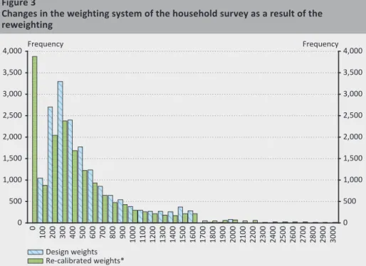
As shown on Figure 3, the initial weights are dispersed in a tighter range [180;
2,100] than the value set of the new weighting (0; 8,000]. Income groups that are over-represented in the HBLS take lower weight values, while groups with a low (weighted) number of observations represent a larger population with higher weights. Apart from weight values close to zero, it is clearly visible that the area21 below the frequency distribution of the original weights is larger than the area marked by the distribution received after the application of the new weights. This is the consequence of the constraint mentioned in sub-section 4.3., namely, that the aggregate number of employees decreases at the level of the national economy due to the reweighting. It is also striking that the occurrence of recalibrated weights above 5,000 is rare, representing employees that are captured with low number in the HBLS, but relatively frequent in tax returns.
Figure 4 illustrates the effect of the reweighting exercise on the income distribution of households. It can be seen that the area below the curve of the frequency
21 The area can be approximated fairly well with the size of the integrals below the kernel density function.
Figure 3
Changes in the weighting system of the household survey as a result of the reweighting
0 500 1,000 1,500 2,000 2,500 3,000 3,500 4,000
0 500 1,000 1,500 2,000 2,500 3,000 3,500 4,000
0 100 200 300 400 500 600 700 800 900 1000 1100 1200 1300 1400 1500 1600 1700 1800 1900 2000 2100 2200 2300 2400 2500 2600 2700 2800 2900 3000
Frequency Frequency
Design weights Re-calibrated weights*
*Note: Although the reweighting also produced weights above 3,000, these are not presented for inter- pretation reasons.
Source: Calculated from HBLS data for 2015 (HCSO 2016)