CORVINUS JOURNAL OF SOCIOLOGY AND SOCIAL POLICY 1 (2011)
INCOME DISTRIBUTION IN NEW (AND OLD) EU MEMBER STATES
István GyörGy tóth1–Márton MedGyesI2
AbstrAct The paper, based on recent EU-SILC data, investigates the patterns of income inequalities in “old” and “new” EU member states. We describe income inequality within countries as well as income differences between states and test our results using different methodological assumptions. Our results show that the group of new member states was no less heterogeneous in terms of inequality and poverty than the EU15 at the time of EU enlargement. The most important difference between the two country groups is found in their GDP levels and in some measures that are directly related to economic development. We observed that sensitivity to changes in the equivalence scales is not systematically related to membership status; thus for overall inequality comparisons of countries, a standard scale seems appropriate. The possibility of a difference between “old”
and “new” EU member states in the role of incomes in generating overall welfare of households calls, however, for caution in interpretation.
Keywords inequality, income distribution, Gini index, SILC
1 ISTVÁN GYÖRGY TÓTH is director of Tárki Social Research Institute, e-mail address:
toth@tarki.hu
2 MÁRTON MEDGYESI is researcher at the Tárki Social Research Institute, e-mail address:
medgyesi@tarki.hu
4 ISTVÁN GYÖRGY TÓTH–MÁRTON MEDGYESI
1. INTRODUCTION AND RESEARCh qUESTIONS3
In 2004 ten new member states joined the European Union. Eight of them were former socialist countries for which accession to the EU ended a 15 year long process of transition from a socialist state to democracy and capitalism.
These were the Central European transition countries (Poland, The Czech Republic, Slovakia, Hungary and Slovenia) and the three Baltic States (Estonia, Lithuania and Latvia)4.
Before the transition, these countries were characterised by relatively low levels of inequality, approximately at the level of Scandinavian societies (Flemming and Micklewright 1999). The transformation of the economy brought about profound changes in these societies, which led to significant increases in inequality and poverty in most of them. The transition economies experienced deep recession at the beginning of the nineties. GDP shrunk by double digits in 1991 in almost all Central and Eastern European countries and the recession continued until the middle of the decade. The Baltic States were particularly heavily affected during this period. In the second half of the nineties the majority of transition countries recovered from recession and continued to enjoy growth rates above the EU average during the period preceding EU accession.
Many studies have sought to analyse the change in inequalities in Eastern European countries during the transition process. For a very careful analysis of trends in earlier years of transition see Flemming and Micklewright (1999).
Milanovic (1999) and The World Bank (2000) give an in-depth analysis of the driving forces behind the evolution of income inequalities in these countries, while Heyns (2005) reviews aspects of increasing inequalities
3 The underlying research for this paper is part of the TARKI (Budapest) research project on income distribution in international comparisons. This version of the paper builds partly upon a longer contribution to the Annual Monitoring Report 2008 of the Network on Social Inclusion and Income Distribution of The European Observatory on the Social Situation (SSO) contracted by DG Employment, Social Affairs and Equal Opportunities Unit E1 (Contract no.
VC/2005/0780) to the consortium of Applica (Be, leader), Essex University (UK), Eurocentre (Vienna) and Tarki. We thank Terry Ward for his generous professional help with previous drafts. Also, we thank András Gábos and Tamás Keller who contributed to previous versions of the analysis. An earlier version of this paper was presented at the Joint OECD/University of Maryland International Conference Measuring Poverty, Income Inequality, and Social Exclusion, Lessons from Europe 16-17 March 2009. We are grateful for the comments we received from the conference participants.
4 We do not have data on Malta and two other countries - Bulgaria and Romania, which joined the EU during the 2007 enlargement. Cyprus – the only new member state not belonging to the group of transition countries – was analysed together with other Mediterranean countries.
CORVINUS JOURNAL OF SOCIOLOGY AND SOCIAL POLICY 1 (2011)
such as inequalities related to gender, age, region of residence, etc. During the economic recession, employment decreased dramatically in transition countries, while unemployment and inactivity were on the rise. The income situation of households which lost employment prospects deteriorated tremendously and this gave rise to a form of inequality previously unknown to them; namely, inequality between those in employment and those working age people who were out of the labour market. Moreover, inequalities between those in employment were also rising during the first phase of transition. As described by Rutkowski (2001), at the beginning of the period the Gini coefficient of earnings inequality fell to the 0,22-0,27 range in these countries. In the first half of the nineties inequality of earnings increased by 4-6 Gini points, while in Lithuania there has been an even more significant increase. During the second half of the decade, earnings inequality continued to increase in most countries. One important factor in increasing earning disparity was an increasing wage premia for educated labourers. Svejnar (1998), Rutkowski (2001) and Kertesi and Köllõ (2002) show that wage premia have considerably increased in every transition country during the nineties. The rise in income inequality was also related to a rising share of entrepreneurial and capital income in household revenues. The emergence of a new private sector and the privatisation of formerly state-owned firms resulted in the formation of a group of corporate business owners.
On the other hand, the eighties and the beginning of the nineties were characterised by increasing inequalities in developed countries as well. Katz and Autor (1999) assert that overall wage inequality and educational wage differentials have been widening significantly in the US, the UK and –albeit more moderately– in the majority of OECD countries since the end of the seventies. It is often argued that increasing earnings inequality in developed countries is the consequence of recent technological changes being skill biased; that is, increasing the demand for educated labour. This might result in an increasing wage premium for education if in the short run the increase in supply is not able to match the increase in demand. Increasing earnings inequality does not translate directly into increasing income inequality, and the evolution of inequalities in disposable household incomes showed more heterogeneous trends, as was demonstrated by the recent OECD report on income distribution (OECD, 2008). Nevertheless, income inequalities did increase in the majority of OECD countries during the period 1985-2005.
In this paper our main objective is to compare the old and the new member states with respect to inequalities in the period of the accession to the EU. The question we ask here is precisely to what extent old and new member states differ according to level of income inequality and poverty. And also: is the
6 ISTVÁN GYÖRGY TÓTH–MÁRTON MEDGYESI
methodology normally used to assess inequalities in the developed countries of the old member states equally valid for analysing inequities in the new member states? We analyse inequalities within countries and we also describe differences in average incomes between countries. We study the effect of methodological choices on our results on inequality and analyse whether changes in methodology have different effects for the old or the new member states. More concretely, we assess the sensitivity of our results to the choice of inequality index and equivalence scale and we also evaluate the effect of sampling errors. Finally, we make an attempt to assess whether our results are influenced by our inability to account for income in-kind due to lack of data.
One of our main findings is that new member states, just like the old member states, are heterogeneous with respect to the level and the dispersion of incomes. To study heterogeneity within these groups we resort to a grouping of countries. Among the old member states we differentiate four groups on the basis of geographic situation but this grouping broadly corresponds also to welfare state types which were described in the literature on welfare states following the work of Esping-Andersen (1990). The country groups we use are Anglo-Saxon countries (Ireland and the UK), Continental countries (Austria, Germany, France, Belgium, the Netherlands, and Luxembourg), Mediterranean (Spain, Italy, Portugal, Greece) and Nordic countries (Sweden, Denmark and Finland).
Recent comparative analyses on inequality in Eastern European countries includes Mitra and Yemtsov (2006) and Bandelj and Mahutga (2010). These studies mainly perform macro-level analysis using inequality data from the UNICEF Transmonee database but without the aim of comparing Eastern European countries to other states. General comparative studies of inequalities, such as OECD (2008) or Brandolini and Smeeding (2009) do provide such information but coverage of Eastern European countries is limited. In these studies comparability of inequality indicators based on different data sources is also an issue. The European Union Study on Income and Living Conditions (EU-SILC) is great step towards reducing these comparability problems. Atkinson et al. (2010) and Ward et al (2009) describe inequalities in EU countries based on EU-SILC data, but with no specific attention given to Eastern European countries. To our knowledge, the only study on transition countries based on data from EU-SILC is Zaidi (2009). This study investigates the role of employment, education and the tax and transfer system in shaping inequality in Central European and Baltic countries. Our study has a different scope however; our aim is to analyse the robustness of inequality comparisons between old and new member states to different choices in inequality measurement. The paper builds on some of our earlier assessments
CORVINUS JOURNAL OF SOCIOLOGY AND SOCIAL POLICY 1 (2011)
of European income distribution (Tóth and Gábos, 2006, Medgyesi, 2008, Medgyesi and Tóth, 2008) and also reflects the work undertaken within the frame of the European Observatory on the Social Situation, Network on Social Inclusion and Income Distribution (see European Commission, 2008a, which is an input to European Commission 2008b).
The extent of poverty and the degree of inequality is shaped by a wide range of factors including the level of economic development, structural factors (employment levels) and social policy factors like the scale of social expenditure and the way that this spent in a given country. There is a great deal of variation among European countries in terms of the mix of institutional factors (and not only in terms of the factors which are capable of being captured in the analysis). The specific circumstances prevailing in any country suggest a need for caution in interpreting the results, especially when drawing policy conclusions. The same policy measures may lead to different results in different countries because of differences in national contexts. Saying more on this would go well beyond the scope of our current paper. Therefore, though we produce and reproduce a number of descriptive statistics on income distribution and poverty in this paper we refrain from making any far-reaching policy suggestions.
The paper is divided into five parts. After this introduction, the second part examines the distribution of income in EU Member States, using standard concepts and assumptions. Part three is devoted to an analysis of the resulting country differences with respect to the use of alternative inequality measures and alternative equivalence scales. Part four goes beyond monetary accounts and attempts to assess the relationship between incomes and the material standard of living in various European countries. Part five concludes.
8 ISTVÁN GYÖRGY TÓTH–MÁRTON MEDGYESI
2. INEqUALITy IN EU COUNTRIES: gENERAL OvERvIEW
Data, concepts and methods
The core of the analysis is based on data from the 2006 EU-SILC5, which covers all Member States, except Malta, for which the ‘microdata’ necessary for the analysis are not available, and Bulgaria and Romania, which initiated surveys only in 2007. In the subsequent graphs we will use abbreviations of country names which are explained in the Annex. These data relate to the population living in private households in the country in question at the time of the survey. Those living in collective households and institutions are, therefore, generally excluded. The income concept used in the analysis is annual net household disposable income, including any social transfers received, and excluding direct taxes and social contributions. The reference period is the year 2005, except for Ireland, where it is the twelve-month period before the date of the interview. We refer to surveys by their fieldwork year (2006) and mention in tables what reference year they correspond to (2005).
Incomes of all household members and other household incomes are aggregated together and total household disposable income is adjusted for differences in household size and composition by use of an equivalence scale to take household economies of scale in consumption into account. As a baseline, we use the so-called modified OECD, or OECD II, scale, which assigns a value of 1 to the first adult in the household, 0.5 to additional members above the age of 14, and 0.3 to children under 14. The equivalised income thus calculated is then assigned to each household member. The inequality indices reported here are estimated on the basis of these figures, except where noted otherwise.
Non-positive income values - which result from the way that the income of the self-employed is defined, i.e. essentially in terms of net trading profits, have been excluded from the analysis. In order to tackle the problem of
‘outliers’ (i.e. extreme levels of income reported), a bottom and top coding procedure (or ’winsorising’) has been carried out (specifically, income values at the bottom of the ranking of less than the 0.1 percentile were replaced by
5 The data used here is taken from EU-SILC (Contract No. EU-SILC 2006/23, signed between TARKI and Eurostat, on 31 January 2007). Appropriateness of the statistical methods of analysis applied to the data and the conclusions drawn from the analyses are the sole responsibility of TARKI; Eurostat and the statistical authorities of individual member states cannot be held responsible. The analyses used the 01/03/2008 version of the EU-SILC 2006/1 database.
CORVINUS JOURNAL OF SOCIOLOGY AND SOCIAL POLICY 1 (2011)
the value of the 0.1 percentile, while at the top of the ranking, values greater than the 99.95 percentile were replaced by the value of this percentile). From among the several indices proposed for inequality measurement6 we use the Gini index7 a baseline for comparisons, while in parts of the analysis we also test other indices with differential capacities to capture various distributional characteristics. For measuring monetary poverty, we use the central “Laeken”
measure: in this way those are considered to be poor whose equivalent income does not exceed sixty percent of the median equivalent income.
In order to draw policy conclusions from inequality and poverty data, it is essential to take account of the fact that the data are derived from surveys of a sample of households and inevitably, therefore, involve some margin of error. To make meaningful comparisons between countries or over time, it is necessary to allow for the margin of error arising from sampling, which can be done by calculating the standard error of the estimates and taking confidence intervals around this. Standard errors for Gini coefficients were derived by the linearization method based on Kovacevic and Binder (1997) and implemented in Stata program “svylorenz” (see Jenkins 2006).
Overall gini rankings
Figure 1. shows the ranking of countries according to the Gini index with standard errors at 95% confidence intervals around the estimates. The Gini coefficient can take values between 0 (complete equality) and 1 (complete inequality); higher values meaning a more unequal distribution. The confidence intervals overlap significantly for many countries, partly because differences in the index are relatively small but also because, for some countries, the standard errors for the index are large. Overlapping confidence intervals make it difficult to establish a precise country ranking. The most that is possible is to define groups of countries, which differ from each other but within which levels are similar.
As Figure 1 shows, countries with the lowest levels of inequality were the Nordic countries Sweden and Denmark, where the Gini index equalled 0,23, and Slovenia was also close to this lowest level, with a Gini value of 0,24. After the countries with the lowest level of inequalities the Continental countries and some Central European countries follow in the country ranking.
6 For reviews of inequality measurement, see for example Cowell (2000). For applications and sensitivity in some CEE countries, see Tóth (2005).
7 = (1/2n(n – 1)) SiSj|yi – yj|, where yi are individual incomes, n is sample size.
10 ISTVÁN GYÖRGY TÓTH–MÁRTON MEDGYESI
Countries with Gini values between 0,25 and 0,26 are the Czech Republic, the Netherlands, Austria, Finland, Germany and Belgium. It is difficult to determine the precise ranking of countries within this group because confidence intervals around our Gini estimates overlap considerably. France, Slovakia, Hungary (in 2004) and Luxembourg show Gini values between 0,27 and 0,28 and also Cyprus has a Gini index of below 0,30. Among countries which recorded a Gini index of over 0,30 we find some Eastern European countries, the Southern European countries (with the exception of Cyprus) and the Anglo-Saxon countries. Spain, Italy, Ireland and the UK have Gini values between 0,30 and 0,32, while the index takes values of between 0,32 and 0,35 in the case of Estonia, Poland, Greece, Lithuania and also in the case of Hungary according to EU-SILC data for year 2005. The highest inequality is seen in Portugal (0,376) and Latvia (0,386).
It might be surprising that Hungary appears three times in Figure 1. We added other estimates of Hungarian inequality in order to illustrate that, in addition to sampling errors, there can be other sources of errors in the cases of some of the countries. It is seen that when observing EU-SILC results from two consecutive surveys, one could think of a huge one-year jump in the level of inequality. While in 2004 Hungary ranked among the middle- inequality countries together with Belgium, Germany and France, in 2005 we measured a 6 point higher Gini index, which ranks Hungary in the upper third of the inequality “league table”. In an alternative survey (the Tarki Household Monitor) the Gini in 2005 is measured to be 29%, which would rank the country among countries with middle-level inequality (Tóth 2008).
This finding may suggest caution in determining the case of other countries as well8.
8 As for Hungary, we exclude the 2005 figure from some of the bivariate analyses and use the 2004 figures instead (most notably, in figures 3 and 4). This follows consultations with CSO officials who notified us pending revisions of the 2006 survey dataset, to be presented when the 2007 survey release becomes available.
CORVINUS JOURNAL OF SOCIOLOGY AND SOCIAL POLICY 1 (2011)
Fig. 1. Gini indices with 95% confidence intervals for EU countries, 2005
Source: EU-SILC 2006. Note: Hu 1: EU-SILC 2006. Hu2: EU-Silc 2005. Hu 3: Tarki Household Monitor 2005.
It is important to note that new member states (NMS) appear across the whole inequality league in Figure 1., with Slovenia and also the Czech Republic belonging to the most equal grouping, the three Baltic states belonging to the most unequal group and the others existing in between. This shows that there is a considerable heterogeneity within the NMS group, being no smaller than the heterogeneity of the EU15 at the time of the enlargement.
Distribution of income in individual European Union member states
In order to have a picture of income differences both between and within countries, we show the distribution of incomes in individual European member states in Figure 2. The income distribution of the countries is represented by the average income of each income decile. The income values are shown in Euros at purchasing power parity (PPP), i.e. with cross-country price differences taken into consideration, allowing direct comparisons to be made.
The countries are arranged in increasing order of average income.
Income differences between countries (in PPS terms) are shown by the relative heights of the bars in Figure 2. The lowest average net disposable
20%
21%
22%
23%
24%
25%
26%
27%
28%
29%
30%
31%
32%
33%
34%
35%
36%
37%
38%
39%
40%
SE DK SI CZ NL AT FI DE BE FR SK HU 2 LU CY HU
3 ES IT IE UK HU
1 EE PL GR LT PT LV
12 ISTVÁN GYÖRGY TÓTH–MÁRTON MEDGYESI
income is in Lithuania (EUR 6024 in PPS terms) and Latvia (EUR 6441 at PPS). Eastern European countries cluster together at the bottom of the scale, with average disposable incomes of under EUR 10,000. The only exception is Slovenia, which ranks higher than Portugal. As is evident, people in the top decile of income distribution in the former socialist countries have an average income that is typical of middle-income earners in most Western European countries (e.g. France or Germany). The highest average income is found to be in Luxembourg (EUR 31,071 at PPS). Average income in the latter is, therefore, near five times that of Lithuania. The largest group of European countries has average incomes between EUR 15,000 and EUR 20,000, and, apart from Luxembourg, the only country where the average level exceeds EUR 20,000 Euros is the UK.
Fig. 2 Income distribution of the countries of the European Union (Euros, PPP)
Source: EU-SILC (2006)
Note: The bottom of the data bars represent the first decile, the top represent the tenth decile and the marks in between show the average incomes of the individual deciles.
0 5000 10000 15000 20000 25000 30000 35000 40000 45000 50000 55000 60000 65000 70000
LT LV PL SK EE HU CZ PT SI GR ES SE IT DE FR FI BE DK NL AT CY IE UK LU
CORVINUS JOURNAL OF SOCIOLOGY AND SOCIAL POLICY 1 (2011)
Inequality and level of economic development
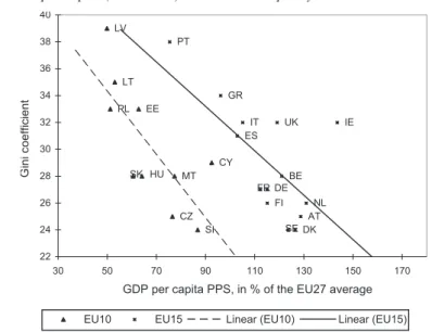
Figure 2 shows, to some extent, the combined effects of the levels and variance of incomes in the various European Union member states. This line of reasoning is extended further in Figures 3 and 4 which present bivariate correlations between relative GDP levels on the one hand and inequality/
poverty levels as measured by Gini indices and by the at-risk-of-poverty rates on the basis of disposable person equivalent incomes of households on the other hand.
Income inequality is relatively strongly and negatively related to GDP per head across the observed EU countries. The slope of the relationship is negative for both the EU15 countries and the New Member States9. There is clearly a large difference between the levels of economic development of the two groups while the internal variance by level of inequality is also large in both subgroups of the EU.
Fig 3. GDP per capita (EU27=100) and income inequality in 2005
SPB Figure 3
2819 2928 1217 2420 3026 1812 1321 2118 2628 1923 2316 2631
26 Figure 4
CZ EE
CY LV
LT
HU MT
PL
SI
SK BE
DK DE
IE GR
ES
FR IT
NL AT PT
FI SE UK
22 24 26 28 30 32 34 36 38 40
30 50 70 90 110 130 150 170
GDP per capita PPS, in % of the EU27 average
Gini coefficient
EU10 EU15 Linear (EU10) Linear (EU15)
CZ EE
CY LV
LT
HU MT PL
SI SK
BE
DK DE
IE GR
ES
FR IT
NL AT PT
FI SE UK
8 10 12 14 16 18 20 22 24
30 50 70 90 110 130 150 170
GDP per capita PPS, in % of the EU27 average
Poverty rate
EU10 EU15 Linear (EU10) Linear (EU15)
Source of data: for Ginis: EU-SILC 2006 and for GDP: EUROSTAT NewCronos Database, download: 1st June, 2008. Variables: GDP PPS 2005 (EU27=100), Gini: 2005 (except for Hungary (2004). “EU15” regression excludes LU.
9 Luxembourg is so much of an outlier that we left it out from the chart for reasons of convenience.
14 ISTVÁN GYÖRGY TÓTH–MÁRTON MEDGYESI
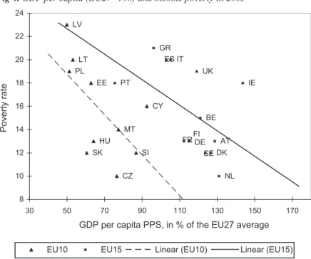
Fig 4. GDP per capita (EU27=100) and income poverty in 2005
Source of data: for poverty rates: EU-SILC 2006 and for GDP: EUROSTAT NewCronos Database, download: 1st of June 2008. Variables: GDP PPS 2005 (EU27=100), At risk of poverty rate (after social transfers) 2005 (except for Hungary (2004). “EU15” regression excludes LU.
The overall risk of poverty is also negatively associated with GDP per head and the pattern of variation across countries is similar. Four groups can be identified10. The first group, containing the Scandinavian countries and most of the EU15 countries with conservative social welfare regimes, has a relatively low overall risk of poverty and a relatively high GDP per head.
The second group, comprising the EU15 Member States with liberal and Mediterranean social welfare regimes, has more variable levels of GDP per head and a relatively high risk of income poverty (around 20%). The other two groups contain the new member states with, in general, a lower level of economic development, but varying levels of relative poverty (some like
10 … and, as a fifth “group”, Luxembourg is an extreme with its high per capita GDP.
SPB Figure 3
2819 2928 1217 2420 3026 1812 1321 2118 2628 1923 2316 2631
26 Figure 4
CZ EE
CY LV
LT
HU MT
PL
SI
SK BE
DK DE
IE GR
ES
FR IT
NL AT PT
FI SE UK
22 24 26 28 30 32 34 36 38 40
30 50 70 90 110 130 150 170
GDP per capita PPS, in % of the EU27 average
Gini coefficient
EU10 EU15 Linear (EU10) Linear (EU15)
CZ EE
CY LV
LT
HU MT PL
SI SK
BE
DK DE
IE GR
ES
FR IT
NL AT PT
FI SE UK
8 10 12 14 16 18 20 22 24
30 50 70 90 110 130 150 170
GDP per capita PPS, in % of the EU27 average
Poverty rate
EU10 EU15 Linear (EU10) Linear (EU15)
CORVINUS JOURNAL OF SOCIOLOGY AND SOCIAL POLICY 1 (2011)
Czech Republic, Slovenia, and Slovakia with lower poverty levels and some like Poland and the Baltic States with lower higher relative poverty levels)11.
Differences in inequalities among old or new member states originate from differences in the dispersion of market incomes and in differences in the inequality-reducing effect of government redistribution. In the group of the EU-15 countries the clustering found here corresponds to degrees of government redistribution. Inequality is lower in countries with a more extensive welfare state; that is, in countries with a Conservative or a Social democratic welfare state. On the other hand, in countries with Liberal and Mediterranean welfare states, where the degree of redistribution is lower, we find higher a level of income inequality.
The NMS were characterised by similar levels of income inequality at the end of the eighties, which where approximately equal to levels of inequality in the Scandinavian countries (Flemming and Micklewright 1999). Of course some heterogeneity existed between the countries, the Czech Republic enjoying a somewhat lower level of inequality, while Poland had higher inequality than the other NMS. During the period of transition, income inequality was on the rise in every NMS due to increasing wage inequality, decreasing employment and a decreasing role of the welfare state in mitigating inequalities. Specificities of the transition process led to a divergence in the level of inequalities. In the Czech Republic and Slovenia the increase in wage inequality and the decrease in employment has been more moderate and consequently these countries ended up with lower levels of inequality (Rutkowski 2001). Among the NMS with higher inequality, Poland and Hungary had a substantial drop in the employment rate, which stabilised at a level as low as 60% and there was an important increase in wage inequality as well. Hungary had to maintain a high degree of redistribution in order to keep income inequality and poverty at a level similar to that of Germany or France. The Baltic States are characterised by higher employment rates than Poland or Hungary, but there has been an important rise in wage inequalities and levels of redistribution are also lower than in the case of Hungary for example (Rutkowski 2001). These led to high levels of income inequality in the Baltic States.
11 We recall here that our current analysis focuses on cross section correlates. In our earlier (Medgyesi and Tóth, 2008) analysis of growth-inequality spells in the EU we concluded that the distributional effects of growth may vary greatly, depending on the nature of growth itself (which sectors drive it, how it affects employment, etc) and the assumed role of social systems (the extent and structure of social expenditure as well as perhaps the social and labour market legislation in place) This accords with the results of recent studies suggesting that the performance of various European social models differ in terms of efficiency and equity (Boeri, 2002) and also with other studies showing that the relationship between growth and inequalities is far from conclusive (Ravallion, 2001, 2004).
16 ISTVÁN GYÖRGY TÓTH–MÁRTON MEDGYESI
3. SENSITIvITy ANALySES
Inequality rankings and the choice of inequality measures
Some inequality indices are particularly sensitive to income changes at the tails of the income distribution. We can therefore expect that indices particularly sensitive to the tails of the distribution would produce rankings that are different form the Gini ranking. We study the ranking according to the P90/P10 index (the ratio of the ninetieth to the tenth percentile of the income distribution), the Squared Coefficient of Variation (SCV)12 index and one member of the Atkinson family of inequality indices13 in addition to the Gini ranking. The SCV index is known to be sensitive to high incomes, while the Atkinson index with inequality aversion parameter ε=2 is very sensitive to low incomes in the distribution (Cowell and Flachaire, 2006).
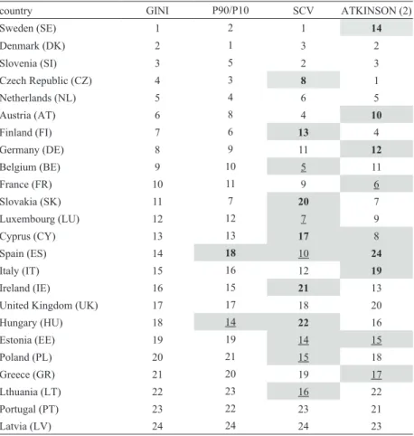
We present the various inequality rank scores of individual countries by various inequality measures in Table 1. The departure from the Gini based to the ranking based on P90/P10 (the ratio of the 90th and the 10th percentile values) does not make a real difference for most countries. If we set a threshold for an important change in the ranking at the movement by at least four steps on the ladder, it is only Spain and Hungary for whom the rankings based on Gini and on P90/P10 would differ from each other. This indifference is not very surprising, however, as both Gini and P90/P10 are “symmetrical”
measures, assigning the same weights to the upper and lower tails of the income distribution. As for the two other measures with an “asymmetric” focus, the changes would be larger. Replacing Gini with SCV would show The Czech Republic, Finland, Slovakia, Cyprus, Ireland and Hungary as being more unequal, while under the same SCV ranking Luxembourg, Spain, Estonia, Poland and Lithuania would be significantly less unequal. Using Atkinson (ε=2) instead of Gini would make Sweden, Austria, Germany, Spain and Italy more unequal while France, Cyprus, Estonia and Greece would be less unequal (as compared to the Gini ranking).
We interpret this sensitivity exercise as a useful way of getting a more balanced picture of inequality patterns across countries. It warns us, for example, that inequality patterns are driven by upper tail changes in some countries like Finland, Ireland and Slovakia, while the inequality is
12 GE(2)=SCV=var(yi)/µ2, where notations are the same as above, and var stands for variance.
13 Atkinson-index: Ae = 1 – [(1/n)Si=1,…,n (yi/m)1–e]1/(1–e), if e ≥ 0 and e = 1 and Ae = 1 – exp[(1/n) Si=1,…,nln(yi/m)], if e = 1, where the notations are the same as above. exp(.)=e(.), and e is the inequality aversion parameter.
CORVINUS JOURNAL OF SOCIOLOGY AND SOCIAL POLICY 1 (2011)
characterised less by the uppermost incomes and rather by the lowest incomes in (say) Sweden or Italy, while in the case of Spain both the upper and lower tails are important in determining the actual inequality patterns. However, changing the measure from one to the other does not have a systematic effect on the “old” or the “new” member states: some new member states would look more unequal while some others would look less unequal when the metric is changed.
Table 1 Rank order of countries by level of inequality as measured by top, middle and bottom sensitive inequality measures
country GINI P90/P10 SCV ATKINSON (2)
Sweden (SE) 1 2 1 14
Denmark (DK) 2 1 3 2
Slovenia (SI) 3 5 2 3
Czech Republic (CZ) 4 3 8 1
Netherlands (NL) 5 4 6 5
Austria (AT) 6 8 4 10
Finland (FI) 7 6 13 4
Germany (DE) 8 9 11 12
Belgium (BE) 9 10 5 11
France (FR) 10 11 9 6
Slovakia (SK) 11 7 20 7
Luxembourg (LU) 12 12 7 9
Cyprus (CY) 13 13 17 8
Spain (ES) 14 18 10 24
Italy (IT) 15 16 12 19
Ireland (IE) 16 15 21 13
United Kingdom (UK) 17 17 18 20
Hungary (HU) 18 14 22 16
Estonia (EE) 19 19 14 15
Poland (PL) 20 21 15 18
Greece (GR) 21 20 19 17
Lthuania (LT) 22 23 16 22
Portugal (PT) 23 22 23 21
Latvia (LV) 24 24 24 23
Note: Cells in grey show a move ofat least 4 rank positions compared to the baseline Gini ranking. (bold: towards higher, underlined: towards lower ranks, when ‘higher rank’ means
‘larger inequality/poverty’).
18 ISTVÁN GYÖRGY TÓTH–MÁRTON MEDGYESI
Inequality rankings and different equivalence scales
Countries differ in terms of typical household size, the number of children per household as well as in terms of the correlation between household size and household income. Therefore changes in the equivalence scale are expected to affect inequality in countries to a different extent. For a simple sensitivity analysis, we compare inequality (Gini) rankings and poverty rate14 rankings when different equivalence scales are utilised. Simple equivalence scales can be defined by raising household size to power e, where parameter e expresses the elasticity of scale in consumption in the household. If e=1 we assume that there is no shared consumption in the household, therefore well-being of household members can be measured by per capita income. An equivalence scale parameter of e=0 equals the assumption that all consumption in the household is shared between members, and the well-being of individuals can be measured by total household income. Values of the e parameter closer to zero express stronger elasticities of scale in consumption. We experiment with values of the elasticity parameter equal to 1, 0.75, 0.5, 0.25 and 0. We also compare estimates obtained by using the OECD II equivalence scale. First we present findings on the sensitivity of the Gini coefficient and the poverty rate related to the choice of the equivalence scale in different country groups.
Finally we compare country rankings according to the Gini coefficient and the poverty rate calculated using the OECD II equivalence scale.
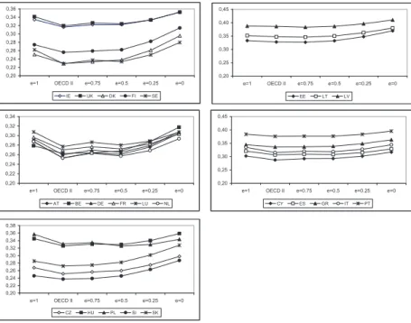
Figure 5 shows the values of the Gini index as the equivalence scale is changed. The graphs show a U-shaped pattern; the Gini coefficient being relatively high for e=1, then lower at e=0.75 equivalence scale. Further decreasing of the elasticity parameter causes the Gini to rise and generally the highest values are obtained when assuming full consumption sharing in the household (e=0)15. Estimates with the OECD II equivalence scale are closest to those obtained with the e=0.75 equivalence parameter. Despite the general U-shaped pattern, the magnitude of changes in the Gini coefficient differs between countries. Among the EU15, the Mediterranean countries seem to be the less sensitive to changes in the equivalence scale. Moderate changes can be detected in the case of France, Luxembourg, the Netherlands and the Anglo-Saxon countries. In the Nordic states and Continental countries such as Germany, Austria and Belgium changing the equivalence scale brings about
14 With a threshold set at sixty percent of the national median income.
15 The U-shaped relationship between the economies of scale parameter and inequality was first empirically demonstrated in the case of the UK in Coulter et al. (1992). Förster (1994) report similar results in an international context, using data from 13 OECD countries.
CORVINUS JOURNAL OF SOCIOLOGY AND SOCIAL POLICY 1 (2011)
more pronounced changes in the Gini: highest Gini exceeds the lowest by at least 20%. The effect of changing the equivalence scale is also different among the NMS. The Czech Republic, Slovakia and Slovenia show more pronounced change, while for the Baltic States, Hungary and Poland changes are moderate.
Patterns of changes in the poverty rate are more heterogeneous (see Figure 6.). In the case of countries like Belgium, Austria, and most of the Western European countries, but also for the NMS of Central-Eastern Europe the U shaped pattern is observable. In other countries like Ireland, Latvia and Portugal we see a pattern of monotonic increase, while in the case of Luxembourg the poverty rate decreases as the equivalence parameter is decreased. Countries also differ in the magnitude of change in the poverty rate. The Netherlands is the country where the poverty rate changes the most with the modification of the equivalence scale. The highest poverty rate, 11,4% (obtained when e=1), is more than the double the lowest value, 4,4% (obtained with the OECDII equivalence scale). In Ireland, Denmark and the Czech Republic the poverty rate is also quite sensitive to changes in the equivalence scale. Less sensitive are Spain, Greece and Italy where the difference between the lowest and the highest poverty rate is below 20%.
We can conclude again that the sensitivity to changes in the equivalence scales is not systematically related to membership status; it affects the old and the new member states as well, without any systematic pattern in this respect.
In Table 2 we examine the change in the ranking of countries using the Gini coefficient and the poverty rate when the equivalence scale is altered.
We compare the rankings obtained with the OECDII and e=0 equivalence scales. When the ranking according to the Gini coefficient is examined, the ranking of countries resembles to a great extent in these two cases. We see important changes only in the case of Austria, Germany and Italy which all move towards the top of the ranking by four or five places. In the case of the poverty rate, Belgium and Estonia move towards the top of the ranking when we switch from the OECDII to the e=0 equivalence scale, while France, Ireland, Lithuania and Greece move towards the bottom of the ranking. Thus changes in country rankings are moderate and changes can both be found among EU15 countries and the NMS.
20 ISTVÁN GYÖRGY TÓTH–MÁRTON MEDGYESI
Figure 5. Sensitivity of Gini estimates to the choice of equivalence scale
0,20 0,22 0,24 0,26 0,28 0,30 0,32 0,34 0,36
e=1 OECD II e=0.75 e=0.5 e=0.25 e=0
IE UK DK FI SE
0,20 0,25 0,30 0,35 0,40 0,45
e=1 OECD II e=0.75 e=0.5 e=0.25 e=0
EE LT LV
0,20 0,22 0,24 0,26 0,28 0,30 0,32 0,34
e=1 OECD II e=0.75 e=0.5 e=0.25 e=0
AT BE DE FR LU NL
0,20 0,25 0,30 0,35 0,40 0,45
e=1 OECD II e=0.75 e=0.5 e=0.25 e=0
CY ES GR IT PT
0,20 0,22 0,24 0,26 0,28 0,30 0,32 0,34 0,36 0,38
e=1 OECD II e=0.75 e=0.5 e=0.25 e=0
CZ HU PL SI SK
CORVINUS JOURNAL OF SOCIOLOGY AND SOCIAL POLICY 1 (2011)
Figure 6. Sensitivity of the poverty rate to the choice of equivalence scale
0,00 0,05 0,10 0,15 0,20 0,25 0,30 0,35
e=1 e=0.75 OECD II e=0.5 e=0.25 e=0
IE UK DK FI SE
0,00 0,05 0,10 0,15 0,20 0,25 0,30 0,35
e=1 e=0.75 OECD II e=0.5 e=0.25 e=0
EE LT LV
0,00 0,05 0,10 0,15 0,20 0,25 0,30
e=1 e=0.75 OECD II e=0.5 e=0.25 e=0
AT BE DE FR LU NL
0,00 0,05 0,10 0,15 0,20 0,25 0,30
e=1 e=0.75 OECD II e=0.5 e=0.25 e=0
CY ES GR IT PT
0,00 0,05 0,10 0,15 0,20 0,25 0,30
e=1 e=0.75 OECD II e=0.5 e=0.25 e=0
CZ HU PL SI SK
22 ISTVÁN GYÖRGY TÓTH–MÁRTON MEDGYESI
Table 2 Rank order of countries by the level of inequalities and poverty as measured by incomes adjusted by different equivalence scales
country
Gini:
OECD II eqscale
Gini:
e=0 country
Poverty ratei:
OECD II eqscale
Poverty ratei:
e=0
Sweden (SE) 1 1 NL 1 2
Denmark (DK) 2 3 CZ 2 1
Slovenia (SI) 3 5 DK 3 4
Czech Republic (CZ) 4 2 SE 4 7
Netherlands (NL) 5 4 SK 5 6
Austria (AT) 6 10 SI 6 5
Finland (FI) 7 6 DE 7 10
Germany (DE) 8 12 FI 8 8
Belgium (BE) 9 8 AT 9 9
France (FR) 10 7 FR 10 3
Slovakia (SK) 11 13 LU 11 13
Luxembourg (LU) 12 9 BE 12 21
Cyprus (CY) 13 11 HU 13 14
Spain (ES) 14 14 CY 14 12
Italy (IT) 15 20 EE 15 20
Ireland (IE) 16 15 IE 16 11
United Kingdom (UK) 17 17 PT 17 17
Hungary (HU) 18 16 UK 18 15
Estonia (EE) 19 18 PL 19 19
Poland (PL) 20 21 IT 20 23
Greece (GR) 21 19 ES 21 22
Lithuania (LT) 22 22 LT 22 16
Portugal (PT) 23 23 GR 23 18
Latvia (LV) 24 24 LV 24 24
Source: own computations based on EU- SILC (2005).
Note: Cells in grey show a move of at least 4 rank places compared to the baseline ranking (bold:
towards higher, underlined: towards lower rankswhere ‘higher rank’ means ‘larger inequality/
poverty’).
CORVINUS JOURNAL OF SOCIOLOGY AND SOCIAL POLICY 1 (2011)
4. ThE ROLE Of INCOMES IN OvERALL WELfARE Of hOUSEhOLDS
So far we have described differences in income inequalities in new and old EU member states. We concluded that new member states form a heterogeneous group with respect to inequalities, just like old member states.
We also demonstrated that changing measurement assumptions does not result in effects which are specific to one or the other country group. Our analysis so far has been based on measures of monetary incomes of households, which did not include incomes in kind, such as consumption of householder-produced items, incomes from owner occupied housing or in kind state intervention (e.g.
provision of public education or health care). The lack of data on income in kind can have an effect on our results since countries might be different with respect to the importance of these income sources. For example: in countries with more extensive welfare state redistribution, in-kind state transfers are more important than for liberal welfare states. In countries where a greater fraction of the population is involved in agriculture, consumption of self- produced food can be more important than in more urbanised and industrialised countries. Countries also differ in the importance of owner occupied housing.
As we lack direct data on these in kind income types, we have tried to assess their importance indirectly: we investigate how strong the relationship is between monetary incomes and measures of material standards of living, such as consumption or wealth. We suppose that the relationship is weaker in countries where income in kind is more important. For example, it might be that in former socialist countries (especially in Central Europe) where owner- occupied housing is important and there is a relatively large rural population involved in subsistence farming, we will find a weaker relationship between income and consumption than for the countries of the EU-15. This would mean that indicators of inequality based only on information about monetary incomes would provide a less reliable picture on actual dispersion of living standards in these countries than in EU-15 countries.
Ideally, this process would involve creating an all-encompassing wealth (or material standard of living) indicator and then we could observe the correlation between income and standard of living or wealth. However, the variable structure of the EU-SILC, unfortunately, is not ideal in this respect.
Although there are some variables on various household goods possessed by the respondents, there are serious limitations to using them as components of a “wealth” index. The information on the (lack of) ownership of cars, washing machines, flushing toilets, etc., in a European context is good for identifying deprivation (i.e. for identifying those NOT having these goods) but it does
24 ISTVÁN GYÖRGY TÓTH–MÁRTON MEDGYESI
not help us to further differentiate between those having these goods (in a European context, these are large segments even in lower income societies).
We therefore tried to experiment with a second best solution to this problem.
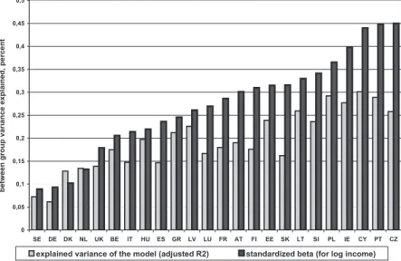
Fig 7. The role of incomes in explaining the variance of the wealth capacity index in EU countries (adjusted R2 and standardized beta for income)
Note: countries are ranked by the value of standardized beta values. Controls: age, education and gender of household head. All beta estimates are significant at p<0.01
We created two indices and called them ‘household wealth capacity index’
and ‘consumption capacity index’. The first (wealth capacity) index contains information on housing conditions16 and on some durables17.
Our first predicted variable (potential household wealth index) is then constructed as a simple, unweighted sum of the z-scores for the possession
16 Rooms per person (variable HH030/HX040), baths (HH080) , flushing toilet (HH090), no leaking roof (HH040), lack of problems with environment (HS180), flat darkness (HS160), crime in surroundings (HS190), noise in the neighbourhood (HS170).
17 Telephone, colour TV, computer, washing machine and car (in EU-SILC variables HS070 HS080 HS090 HS100 HS110 respectively).
gfig7
1. oldal 0,00
0,05 0,10 0,15 0,20 0,25 0,30 0,35 0,40
DK NL ES UK GR SE DE IT SK HU AT LU FR BE IE SI FI CY EE PL LV PT CZ LT
between group variance explained, percent
explained variance of the model (adjusted R2) standardized beta (for log income)
CORVINUS JOURNAL OF SOCIOLOGY AND SOCIAL POLICY 1 (2011)
of the above-mentioned (thirteen) items about housing conditions and possession of durables. The further away an individual is from the centre of the distribution, the higher the (positive or negative) value of the index will be. We assumed that higher parameter estimates of (natural logarithm of net person equivalent) disposable income would signal that income has stronger explanatory effect on wealth capacity. While running the OLS regressions for the predictions, we controlled for age (four brackets: -35, 36-49, 50-64 and 65+), education (less than secondary, secondary and tertiary) and gender of household head18. The standardized beta coefficients of income and the explained variance of the models are shown in Figure 7. We see from the figure that lower levels of GDP (in the “West” and the “East” as well) tend to be associated (with some exceptions) with the larger role of income in explaining the variance of the wealth capacity index.
Fig 8. The role of incomes in explaining the variance of the consumption capacity index in the EU countries (adjusted R2 and standardized beta for income)
Note: countries are ranked by the value of the standardized beta values. Controls: age, education and gender of household head. All beta estimates are significant at p<0.01
18 The regressions were run taking households as units.
0 0,05 0,1 0,15 0,2 0,25 0,3 0,35 0,4 0,45 0,5
SE DE DK NL UK BE IT HU ES GR LV LU FR AT FI EE SK LT SI PL IE CY PT CZ
between group variance explained, percent
explained variance of the model (adjusted R2) standardized beta (for log income)
26 ISTVÁN GYÖRGY TÓTH–MÁRTON MEDGYESI
The other predicted index variable we constructed comprises several consumption ability items19 for which we constructed the same type of z-score based indices and predicted these in the same type OLS regressions (using the same controls) as above. Standardized beta coefficients for the consumption capacity index are shown in Figure 8. Conclusions are very similar as the figure shows similar country rankings but slightly higher parameter estimates.
We again see new member states with relatively high explanatory power of income on the consumption capacity index and also the explained variance of the models is larger. These findings suggest that the correlation between monetary income and indicators of standard of living is not weaker in the new member states than in the EU15 countries. Actually, it appears that monetary income predicts more closely living standards in the new member states.
Our hypothesis to explain the above findings includes both methodological and substantive comments. The first come largely from the fact that the index we constructed is made of those goods and housing conditions that are designed to measure deprivation. The higher is the GDP in a country, the higher is the penetration of the ownership of these durables. Therefore, the correlation between income and durable ownership tends to be higher in lower GDP countries. As an illustrative example, we show on the following graph (Figure 9.) the percentage of households having a personal computer in the different income quintiles, in the case of a country with a high penetration ratio (Netherlands) and in a country with relatively low penetration (The Czech Republic). In the high penetration country, differences in PC ownership according to income are much smaller than in the country with lower penetration. This difference is not a consequence of greater income differences among the quintiles in the lower penetration country. The two countries, the Netherlands and the Czech Republic, are quite similar with respect to the extent of income inequalities as the similarity of the relative income lines show. In the case of the Netherlands, higher absolute income level results in higher penetration, which leads to a weaker relationship between income and durable ownership. We assume this holds for many items that are included in our index and hence in countries with lower level of GDP (and consequently, a lower penetration of various goods) the relationship between the index (as constructed this way) and incomes appears stronger.
19 The answer to the question on ability to make ends meet (variable HS120, six categories, from very easily to “with great difficulty”), the ability to pay for an unexpected expense (variable HS060 at the level of 1/12 of the poverty threshold for a household on average), or the ability to pay for a week’s holiday away from home (HS040) and the ability to keep home adequately warm (HH050).
CORVINUS JOURNAL OF SOCIOLOGY AND SOCIAL POLICY 1 (2011)
Also, participation in the informal economy may lead to distortions when estimating the correlation of income and material well-being. The direction of the distortions, however, is uncertain, as informal pay received may render measured income underestimated, while informally bought goods (like used cars or televisions) may mean cheaper access to durables. However, at this current stage we cannot go further in elaborating on these speculations (due to lack of adequate data on both in-kind and informal payments).
Fig 9. Percentage of households with a personal computer (left axis) and relative income (right axis) by income quintiles in the Netherlands and in The Czech Republic)
Note: Income quintiles are based on the household-level distribution of household equivalent income. Relative income is calculated relative to country mean income.
5. SUMMARy AND CONCLUSIONS
We analysed income distribution patterns of the European Union countries, based on the EU-SILC survey (reflecting incomes in 2005). We first charted overall distributional patterns, followed by sensitivity analyses with respect to various inequality measures and two different equivalence scales. We found a considerable degree of heterogeneity among the EU countries both in the level of GDP and in the measured dispersion of incomes. While the NMSs have much lower GDP per head, even in PPS terms there are, in general, no
0%
10%
20%
30%
40%
50%
60%
70%
80%
90%
100%
1. quintile 2 3 4 5. quintile
0,0 0,5 1,0 1,5 2,0 2,5 3,0
NL, % of PC owners CZ, % of PC owners
NL, relative income (right axis) CZ, relative income (right axis)