MŰHELYTANULMÁNYOK DISCUSSION PAPERS
INSTITUTE OF ECONOMICS, CENTRE FOR ECONOMIC AND REGIONAL STUDIES,
MT-DP – 2019/16
Convergence, productivity and debt:
the case of Hungary
DÁNIEL BAKSA – ISTVÁN KÓNYA
Discussion papers MT-DP – 2019/16
Institute of Economics, Centre for Economic and Regional Studies, Hungarian Academy of Sciences
KTI/IE Discussion Papers are circulated to promote discussion and provoque comments.
Any references to discussion papers should clearly state that the paper is preliminary.
Materials published in this series may subject to further publication.
Convergence, productivity and debt: the case of Hungary
Authors:
Dániel Baksa macroeconomist
Institute for Capacity Development
International Monetary Fund and Central European University dbaksa2@IMF.org
István Kónya research advisor Institute of Economics
Centre for Economic and Regional Studies, University of Pécs and Central European University
konya.istvan@krtk.mta.hu
September 2019
Convergence, productivity and debt:
the case of Hungary
Dániel Baksa – István Kónya
Abstract
We study the role of productivity convergence and financial conditions in the recent growth experience of Hungary. We build a stochastic, small-open economy growth model with productivity convergence, capital accumulation and external borrowing. Using empirically identified processes for productivity and the external interest premium, we simulate the effects of two unexpected, permanent changes on Hungarian growth. The first change is the sharp productivity slowdown starting in 2006, and the second is the tightening of external financial conditions starting in 2009. Simulating our model, we show that the empirically identified productivity and interest premium processes - along with the two unexpected permanent changes and regular i.i.d. productivity and interest premium innovations – capture the main medium-run dynamics of the Hungarian economy both before and after the global financial crisis. Running counterfactuals, we also find that the observed slowdown in GDP per capita growth was mostly driven by productivity, while the tightening of external financing conditions is important to understand investment behavior and the net foreign asset position.
Keywords: economic growth, convergence, productivity, interest premium, Hungary
JEL classification: E13, E22, F43, O47
Acknowledgement: This research was supported by: (1) the Higher Education Institutional Excellence Program of the Ministry for Innovation and Technology in the framework of the “Financial and Public Services” research project (temporary reference number: TUDFO/47138-1/2019-ITM) at Corvinus University of Budapest, and (2) The National Research, Development and Innovation O_ce of Hungary (OTKA K116033).
Konvergencia, termelékenység és adósság:
magyar tapasztalatok
Baksa Dániel – Kónya István
Összefoglaló
A tanulmány azt vizsgálja, hogy milyen szerepet játszott a termelékenységnövekedés és a pénzügyi környezet az elmúlt évek magyar gazdasági növekedésében. Ehhez egy sztochasztikus, kis nyitott gazdaságot feltételező modellt építünk, amelyben megjelenik a tőkefelhalmozás, a felzárkózó termelékenység, illetve a külső adósság. Empirikusan identifikált termelékenységi és kamatprémium-folyamatokat felhasználva két váratlan, tartós sokk magyar gazdaságra gyakorolt hatását szimuláljuk a modell segítségével. Az első változás a termelékenységi felzárkózás erős lelassulása 2006-tól, a második pedig a külső pénzügyi feltételek 2009-ben kezdődő szigorodása. A modellszimulációk azt mutatják, hogy az empirikusan identifikált termelékenységi és kamatprémium-folyamatok – a két váratlan, tartós változással és a rendszeresen érkező f.a.e. termelékenységi és kamatprémium- sokkokkal együtt – jól magyarázzák a magyar gazdasági növekedés középtávú dinamikáját mind a globális pénzügyi válság előtt, mind pedig azután. Tényellenes szimulációk segítségével azt is megmutatjuk, hogy az egy főre jutó GDP növekedésének megfigyelt lassulását főként a termelékenység magyarázza, míg a külső pénzügyi környezet szigorodása fontos szerepet játszott a beruházás és a nettó külföldi pozíció alakulásában.
Tárgyszavak: gazdasági növekedés, konvergencia, termelékenység, kamatprémium, Magyarország
JEL kódok: E13, E22, F43, O47
Convergence, productivity and debt: the case of Hungary
∗Dániel Baksa† István Kónya‡ August 2019
Abstract
We study the role of productivity convergence and financial conditions in the recent growth experience of Hungary. We build a stochastic, small-open economy growth model with productivity convergence, capital accumulation and external borrowing. Using empiri- cally identified processes for productivity and the external interest premium, we simulate the effects of two unexpected, permanent changes on Hungarian growth. The first change is the sharp productivity slowdown starting in 2006, and the second is the tightening of external financial conditions starting in 2009. Simulating our model, we show that the empirically identified productivity and interest premium processes - along with the two unexpected permanent changes and regular i.i.d. productivity and interest premium innovations - cap- ture the main medium-run dynamics of the Hungarian economy both before and after the global financial crisis. Running counterfactuals, we also find that the observed slowdown in GDP per capita growth was mostly driven by productivity, while the tightening of external financing conditions is important to understand investment behavior and the net foreign asset position.
Keywords: economic growth, convergence, productivity, interest premium, Hungary.
JEL: E13, E22, F43, O47
∗This research was supported by: (1) the Higher Education Institutional Excellence Program of the Ministry for Innovation and Technology in the framework of the “Financial and Public Services” research project (temporary reference number: TUDFO/47138-1/2019-ITM) at Corvinus University of Budapest, and (2) The National Research, Development and Innovation Office of Hungary (OTKA K116033).
†Institute for Capacity Development, International Monetary Fund and Central European University. E-mail:
dbaksa2@IMF.org
‡Centre for Economic and Regional Studies, University of Pécs and Central European University. Corresponding author, e-mail: konya.istvan@krtk.mta.hu.
1 Introduction
Neoclassical growth theory predicts conditional convergence, which means that a country that starts below its long-run level of capital will grow faster for a while. The prediction also applies when there is fast productivity increase due to the importing of better technologies, organization practices, or institutions. The so-called new member states of the European Union have expe- rienced convergence for a combination of these reasons after the initial transition recessions of the early 1990s.
The same is true for Hungary, whose GDP per capita has risen from below 50% of the German level in 1995 to about 64% in 2016, calculated at current purchasing power parities. The speed of convergence, however, has been very uneven. After a brief slowdown in 1996, Hungarian growth was strong until 2006. Afterwards, however, convergence stopped for almost a decade, partly due to the global financial and subsequent Euro crises between 2008-2012. Growth resumed after 2012, and Hungary is again on an income convergence path. As we show below, however, the recent pick up in GDP per capita growth has been driven mostly by increases in employment. If one focuses on GDP per hours worked, growth has still not returned to pre 2006 levels.
In this paper we study two possible explanations for the slowdown in Hungarian growth.
The first explanation is a productivity growth decline, and the second is a credit crunch. Using empirical measures of total factor productivity and the sovereign interest premium, we docu- ment that both explanations are qualitatively consistent with events after 2006. The question is whether the productivity or finance based explanations - individually or jointly - are able to explain the Hungarian growth experience quantitatively.
To evaluate this we build a small-open economy, neoclassical growth model with capital accumulation, productivity convergence and a debt-dependent interest rate. We calibrate the model to the Hungarian economy, and simulate the effects of two unexpected permanent shocks.
The first is a slowdown in the rate of productivity convergence, and the second is an increase in the debt elasticity of the interest rate on foreign borrowing. We discipline the exercise by using empirically identified processes for both productivity (using the Solow residual), and for the interest premium (using EMBI spreads).
Our results show that these two shocks are able to explain the major medium-term features of the Hungarian growth experience. The model does a good job at matching growth facts both
before and after the shocks hit. We find that overall slow growth has been driven by TFP, but the behavior of investment and the net foreign asset position cannot be understood without the sustained increase in the interest premium.
Our paper is related to articles that study the roles of productivity vs. finance in explaining growth volatility in emerging economies. Aguiar and Gopinath (2007) stress the role of growth shocks to explain the cyclical behavior of consumption and the trade balance. Estimating the neoclassical model on Argentine data, García-Cicco, Pancrazi and Uribe (2010) find that interest premium shocks seem to be more important drivers of the Argentine experience. Subsequent papers found different results for different countries. Naoussi and Tripier (2013) and Guerron- Quintana (2013) find that shocks to trend productivity are more important to explain growth volatility in African countries than financial shocks. For the so-called Visegrad countries of the Czech Republic, Hungary, Poland and Slovakia, Baksa and Kónya (2017) also confirms the primary role of productivity shocks. In contrast, Tastan (2013) finds that in Turkey financial shocks are more important.
We contribute to this literature using a somewhat different modeling approach. While we also rely on the neoclassical growth model, we focus on medium-term convergence instead of short- run cyclicality. Our goal is to understand the fast convergence and subsequent sharp slowdown in Hungary in a unified framework. Given our emphasis on convergence, we use the original, non-linear version of the model, since linearized solutions are inaccurate when a country is far from its steady state. We use theextended pathsolution method (Gagnon, 1990), which relies on a series of deterministic simulations enhanced by unexpected temporary and permanent shocks.
We also differ from the literature in that we use identified processes for the interest pre- mium and productivity as the main driving forces of the model. This is especially important for the interest premium, which is typically identified from the behavior of consumption and the trade balance in estimated linearized models (García-Cicco, Pancrazi and Uribe 2010). Using an observed interest premium series puts additional discipline on the model, providing external val- idation for the results. We also provide a useful and highly tractable alternative to estimation.
Using only two observed shock processes we keep the model simple and transparent, while still making it empirically grounded. The disadvantage is that we cannot perform formal statistical tests. On the other hand, Hungarian time series are short, so the power of such tests is low. Our approach yields important insights when estimation is either not feasible or not reliable.
The rest of the paper is structured as follows. Section 2 provides a brief overview of the Hungarian growth experience between 1995-2018. Section 3 builds the model used for subse- quent simulations. Section 4 details the choice of model parameters and the identification of the productivity and interest premium processes. Section 5 describes the simulation exercise and presents the results. Finally, Section 6 concludes.
2 Convergence in Hungary
In this section we present a few basic facts about Hungarian growth between 1995-2017. Due to data limitations, we will later restrict attention to the sub-period 1999-2016. Looking at the earlier years of 1995-1998, however, adds useful context to the subsequent period. Also note that the transition recession in Hungary lasted between 1990-1993, and there was substantial fiscal adjustment in 1996. By 1999, however, the Hungarian economy was along what was then thought to be a fast, sustainable convergence path.
1995 2000 2005 2010 2015 2020 -6
-4 -2 0 2 4
% change
Real GDP growth
1995 2000 2005 2010 2015 2020 18
20 22 24 26
% GDP
Investment rate
1995 2000 2005 2010 2015 2020 -120
-110 -100 -90 -80 -70 -60
% GDP
Net foreign asset position 1995 2000 2005 2010 2015 2020 4000
4100 4200 4300 4400 4500 4600
Thousand persons
Employment
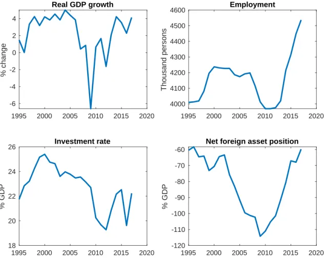
Figure 1: Hungarian growth facts, 1995-2017
Figure 1 plots four indicators for the Hungarian economy: the growth rate of real GDP, the employment rate, the investment rate and the net foreign asset position. The beginning of the period is characterized by increasing growth, employment and investment, and a slowly deteri- orating external investment position (driven primarily by foreign direct investment inflows).
The second period, between about 2000-2005 is characterized by high growth, stable employ- ment, slowing investment, and a dramatic worsening of the net foreign asset position (driven primarily by public and private debt). The period between 2006-2013 is a long recession, with low or negative growth rates, a large decline in investment and employment, and external re- balancing. Our main focus in this paper is no these two periods, first with fast convergence increasingly driven by a credit boom, and then a massive slowdown accompanied by significant external adjustment.
Finally, the years between 2014-2017 saw a return to higher growth rates, accompanied by higher but erratic investment rates, and by continuing balance sheet adjustment. Note that the last period is also characterized by a large and sustained increase in employment. We show later that productivity growth in Hungary is still disappointingly low. These two developments may be partly explained by the fact that a significant part of employment growth is in public works projects, whose economic value is questionably (Fazekas and Varga, 2015). While investment is recovering, it is to a significant degree driven by European Union structural funds (Baksa and Kónya, 2017) and government investment. The effects of EU funding can be seen in 2016, when there was a temporary lull in inflows.
Arguably Hungary is returning to a faster convergence path in 2017-2018. Employment growth is increasingly driven by the private sector, and corporate investment is picking up. On the other hand, the country is experiencing a housing boom along with quickly increasing hous- ing prices. Since our data used in the subsequent sections ends in 2016, we do not need to take a stand on the sustainability of the current high growth rates.
As we explained in the Introduction, we focus on the roles of productivity growth and the external financial environment measured by the foreign interest premium. In what follows we ignore two additional drivers of Hungarian growth. The first is fiscal policy, which was thought to be behind the slowdown of GDP growth in 2006. It is difficult to model fiscal policy realistically in the neoclassical framework, and there are signs that the impact of the fiscal adjustment would have been temporary in the absence of the global financial crisis starting in 2008.
Second, we ignore employment and focus on labor productivity in our model. The increase in employment starting in 2013 is at least partly driven by government policy targeting labor supply, which would add an additional exogenous driving force to the model (at least between 2013-2016). While it would be desirable for our model to endogenously generate the large decline in employment in 2009, it turns out to be difficult to model the labor market in a way that matches both its cyclical component and its convergence behavior. We do use employment and hours in the measurement of total factor productivity, but we leave the proper modeling of labor supply for future research.
3 The model
The model is a variant of the small open economy neoclassical growth model. We work with the sequential markets, decentralized version of the model, which facilitates the calibration exercise later. Households consume, invest and save. A discount bond is available through which house- holds can borrow and save on international financial markets. Firms borrow capital and labor from households on competitive factor markets, and sell them a single consumption/investment final good, also on a competitive market. We normalize the price of the final good to unity, and useWtandrkt to denote the wage rate and the rental rate of capital, respectively.
3.1 Households and firms
The representative household solves the following inter-temporal problem:
maxEt
∞
X
t=0
βtlogCt
s.t. Bt+1
Rt −Bt=WtNt+rktKt−Ct−It Kt+1 = (1−δ)Kt+
"
1−φ 2
It gIt−1
−1 2#
It,
whereCtis consumption,Btis the amount of foreign bonds that matures att,Ntis the supply of labor,Kt is the stock of physical capital available for production att, andItis investment.
Capital accumulation is subject to investment adjustment costs as in Christiano, Eichenbaum
and Evans (2005). We choose this specification instead of capital adjustment costs because it can account for the gradual response of investment in response to shocks. Since the model will have a balanced growth path where the common growth rate isg, we write the investment cost function such that it is zero along the BGP. We assume that households have a time endowment of1, and since they do not value leisure, labor supply isNt= 1.
The first-order conditions of the problem are straightforward, and are given as
1 Ct
=βRtEt
1 Ct+1
qt= 1 +φ 2
It
gIt−1
−1 2
+φ It
gIt−1
−1 It
gIt−1
−βφEt
It+1
gIt −1 It+1 gIt
2
Ct Ct+1qt+1 qt=βEt
h
rt+1k + (1−δ)qt+1
i Ct
Ct+1.
The first equation is the Euler equation corresponding to foreign bonds. The second equation describes the evolution of investment. The third condition is the arbitrage between bond and capital investment.
Firms produce with a standard Cobb-Douglas production function using capital and labor:
Yt=etAtKtα(XtNt)1−α.
We assume that productivity has three components. First, Xt stands for deterministic, labor augmenting productivity that grows at the gross rate ofg = Xt/Xt−1. Second, we allow for catch-up productivity growth towards the steady state, captured by the termAt. Given an initial levelA0, this term follows and exogenous, autoregressive process:
at=ρtat−1, (1)
whereat = logAt and as we discuss later, we allow the convergence coefficientρ to change over time. Finally, we allow for a stochastic shockt, which is assumed to be an i.i.d. white noise process.
The crucial - and nonstandard - component in this setup is the convergence termat. We use
this specification to allow for transition growth apart from capital accumulation. Many authors have documented that the main reason for underdevelopment is low productivity (Caselli, 2005;
Hall and Jones, 1999; Kónya, 2018). Since explicitly modeling the diffusion of knowledge would be complicated, we simply assume an exogenous process. The important assumption is that this is known by agents, and productivity catch-up is built into expectations. In our main exercise one of the key shocks to hit the economy is an unexpected, permanent change in this process.
The first-order conditions are again straightforward, and are given by
rtk=α Kt
XtNt
α−1
Wt= (1−α)Xt
Kt
XtNt α
.
Both labor and capital are employed so that their marginal products equal their price.
3.2 Equilibrium
It is well-known that with an exogenous interest rate small open economy models are not sta- tionary. We follow the literature (Schmitt-Grohé and Uribe, 2003) and assume that the interest rateRtdepends on the net foreign asset position as follows:
Rt= g βeυt υt=ρrυt−1−ψt
Bt
Yt −by
+rt, (2)
whereυtis the interest premiumbyis the long-run, exogenously given sustainable debt position, andψis the debt elasticity of the interest premium (which can change over time). Note that we deviate from the typical specification in two ways. First, we use the NFA/GDP position (as opposed to the NFA level) as a measure of indebtedness. This is mostly innocuous, but we think it is closer to the idea that the premium captures (in a reduced form way) the perceived probability of default. Second, we add an autoregressive term to the premium function. This will to capture the fact that the Hungarian interest premium was declining during the early 2000s, while the NFA position was worsening. This can be explained by our specification with an initial premium that is above its level conditional on indebtedness. Note that we set the steady state level of the
external interest rate to coincide with the implicit domestic one.
Since productivity has a deterministic trend, we normalize growing variables by the growth factorXt. Letct =Ct/Xt,it =It/Xt,kt =Kt/Xt,bt =Bt/Xtandyt =Yt/Xt. Combining the household and firm conditions and using the normalized variables, we get the following conditions:
1 =eυtEt
ct ct+1
qt= 1 +φ 2
it it−1
−1 2
+φ it
it−1
−1 it
it−1
−β gφEt
it+1 it
−1 it+1 it
2
ct ct+1
qt+1
qt= β gEt
αyt+1
kt+1
+ (1−δ)qt+1
ct
ct+1
gkt+1 = (1−δ)kt+
"
1−φ 2
it
it−1
−1 2#
it (3)
βe−υtbt+1 =yt+bt−ct−it yt=eteatktα
υt=ρrυt−1−ψ bt
yt−by
+rt rtk= αyt
kt
wt= (1−α)y Rt= g
βeυt
The set of equations (3) characterize the competitive equilibrium for the price sequences{υt}∞t=0, {Rt}∞t=0, ,
rtk ∞t=0, {wt}∞t=0, {qt}∞t=0 and the allocation sequences {ct}∞t=0, {it}∞t=0, {kt}∞t=0, {bt}∞t=0,{yt}∞t=0. Initial conditions for the endogenous and exogenous state variables are given byk0, b0, υt, a0. It is easy to show (see next section) that there is a unique, deterministic steady state to which the system would converge in the absence of stochastic shocks.
4 Calibration and shock processes
The model economy is driven by (i) convergence dynamics due to capital accumulation and pro- ductivity convergence, and (ii) exogenous shocks to productivity and the interest premium. One of the main contributions of our paper is that empirically observed processes for productivity and the interest premium generate convergence dynamics in line with the data. In this section we detail the choice of the model parameters and the identification of the two processes.
4.1 Data
We use the following annual time series for the Hungarian economy between 1999-2016.
GDP Chain linked gross domestic product, base year 2011. Source: Eurotat.
Investment Gross fixed capital formation, chain linked, base year 2011. Source: Eurostat Capital stock Total (net) fixed assets at current replacement cost. Source: Eurostat Net foreign assets Net foreign asset position as a percentage of GDP. Source: Eurostat Interest premium JP Morgan Emerging Markets Bond Indicator (EMBI) spread. Source: World
Bank
Population Total population. Source: Penn World Table
Employment Total employment, national accounts, domestic concept. Source: Penn World Table
Average hours Annual hours worked per worker. Source: Penn World Table
Capacity utilization Capacity utilization in the manufacturing sector. Source: Eurostat Workfare employment Number of workers in public workfare programs. Source: Eurostat,
Hungarian Statistical Office.
Adjusted labor share Compensation of employees relative to value added, adjusted with the number of self-employed. Source: AMECO.
There are a number of issues that arise when using the data above. First, the measurement of the capital stock is problematic. This is documented in many papers, and authors often choose
to compile their own capital stock estimates using the perpetual inventory method (PIM). In the context of Hungary and other transition economies, however, the choice of an initial capital stock (which is necessary for the PIM procedure) is far from innocuous. A recent paper (Levenko, Oja and Staehr, 2019) highlights many of the issues that arise in Eastern European economies, and presents its own estimates. While the levels are different, Figure A1 in their paper shows that the dynamics of the capital-output ratio are very similar across the authors’ estimates, and publicly available data from the Eurostat and AMECO. Since for the calculation of total factor productivity growth only the dynamics matter, we simply work with the Eurostat series. Apart from being publicly available, another advantage of the Eurostat series is that it is consistent with data on the labor share (see the next section). The only limitation is that data ends in 2016, so this is the last year we can include in our sample.
Total factor productivity measurement also needs labor input. We rely on the Penn World Ta- ble for employment and hours worked. We use the PWT because hours worked in Eurostat have a structural break in 2010, when there is a one-time, steep drop in the series. This is acknowl- edged by the Hungarian Statistical Office, but they do not calculate hours before the break with the new methodology. The Penn World Table average hours do not have this problem, implying that there is an adjustment in the PWT that corrects for the break.
In addition to hours, the measurement of total employment is also problematic. After 2010 the number of people participating in workfare programs has increased significantly, reaching a peak of about 5% of total employment by 2015. There is a strong perception that Hungarian workfare jobs are unproductive (Fazekas and Varga, 2015). They tend to involve people with very low skills, and employ them in a way that contributes very little to GDP. The workfare scheme is essentially a social program, so we simply subtract these people from the employment statistics.
Capacity utilization is important for the calculation of productivity (Basu, 1996). Unfortu- nately, there is no economy-wide utilization measure, but Eurostat reports utilization for man- ufacturing. It is possible to use other proxies (Kónya, 2018), but here we follow Levenko at al.
(2019) and simply assume that the manufacturing statistics applies to the broader economy.
Finally, we use EMBI spreads to measure the external interest premium. There are alternative indicators, such as sovereign CDS spreads, or domestic interest rates corrected by inflation or exchange rate changes. The advantage of the EMBI over CDS spreads is that for Hungary the time series is longer, starting in 1999. Relative to domestic currency denominated assets, its main
advantage is that it compares assets denominated in US dollars, so that exchange rate risk is not an issue.
4.2 Calibration
For some of the parameters we choose values commonly used in the literature. In particular we set the discount factor toβ = 0.96, the depreciation rate toδ = 0.05 and the investment adjustment cost parameter toφ = 10. Without loss of generality, we normalize the long run level of productivity toa¯= 1. The long run sustainable NFA/GDP position is set toby = 0, since there is no obvious alternative value for the Hungarian economy and cross-country evidence is also inconclusive.
We set the long-run growth rate to0.01, which equals the average growth rate of GDP per hours worked in Germany between 1995-2018. The capital elasticity of the production function is set toα= 0.4, which equals one minus the adjusted labor share for the same period in Hungary.
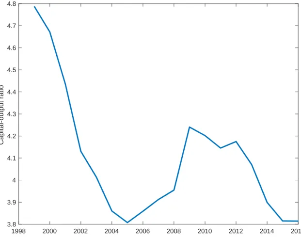
Using the set of equilibrium conditions (3), it is easy to see that the capital-output ratio is given by the steady state equations as
¯k
¯
y = α
g/β−1 +δ.
Given our calibration, this value equals ¯k/¯y = 3.98. Figure 2 plots the capital-output ratio from Eurostat. It is significantly higher during the first two years of the sample period, but than fluctuates around4, which is the steady state value we just calculated. The fact that Hungary started the period with a higher capital-output ratio might sound counterintuitive at first. Notice, however, that many Eastern European economies were highly capital intensive during the period of central planning. Therefore, it is not implausible that the capital-output ratio was still declining in the first decade of transition.
4.3 Shock identification
We use two empirically identified shock processes as exogenous model drivers. In this section we detail how the productivity and premium processes are recovered from the data. Our main exercise is to feed unexpected, permanent changes in these processes into our theoretical model.
1998 2000 2002 2004 2006 2008 2010 2012 2014 2016 3.8
3.9 4 4.1 4.2 4.3 4.4 4.5 4.6 4.7 4.8
Capital-output ratio
Figure 2: The capital-output ratio in Hungary
Therefore, we need to find the breaks in the productivity and the premium sequences. As it turns out, the data is very clear about breaks and we simply identify them by visual inspection. We start with the components of productivity, and then turn to the interest premium.
4.3.1 Total factor productivity
We calculate total factor productivity as the Solow residual. Recall that total factor productivity in our framework is defined as
T F Pt=etAtXt1−α.
We can rewrite the production function to express TFP as a function of labor productivity to the capital-output ratio:
T F Pt= (Yt/Nt)1−α (Kt/Yt)α .
To calculate TFP, we use the following augmented productivity function:
Ytobs =T F Pt×
uobst Ktobsα
hobst Lobst 1−α
,
whereutis capacity utilization,htis annual hours per worker, andLtis employment. Although these are not modeled explicitly, they are important for the measurement exercise. Our aim is not to reproduce the exact movements in output, but to see how it evolves over time given changes in its long-run driver, productivity.
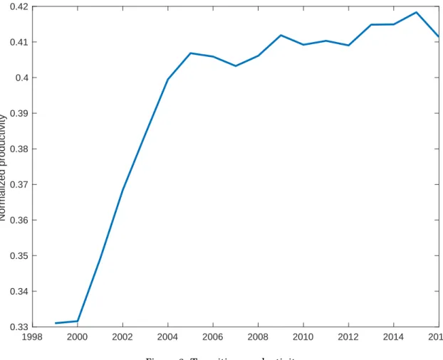
Once we identify the TFP series, we calculate the three components the following way. First, the deterministic trend is simply given byXt = gt, since we normalizeX0 = 1. We create a normalized series by dividing TFP withXt1−α. This series is depicted on Figure 3.1It is clear that there are two distinct regimes in Hungarian productivity convergence. The first regime lasts until 2005, and it is characterized by fast convergence. The second regime starts in 2006 and is characterized by slow convergence.
To fit these two periods, we use the specification of theAtprocess given in eq. (1), and solve forAt = A0ρt.Then we simply use nonlinear least squares on the two subsamples 1999:2005 and 2006:2016 to find the convergence parameters ρ1 = 0.962andρ2 = 0.997. Notice that the productivity slowdown occurs before the global financial crisis. We experimented with a cutoff date of 2008, but the productivity fit in that case is obviously much worse. Also note that controlling for hours and capacity utilization are sufficient to eliminate a large fall in productivity in 2009. This is an important reason to include these controls, since large falls in exogenous productivity are difficult to explain.
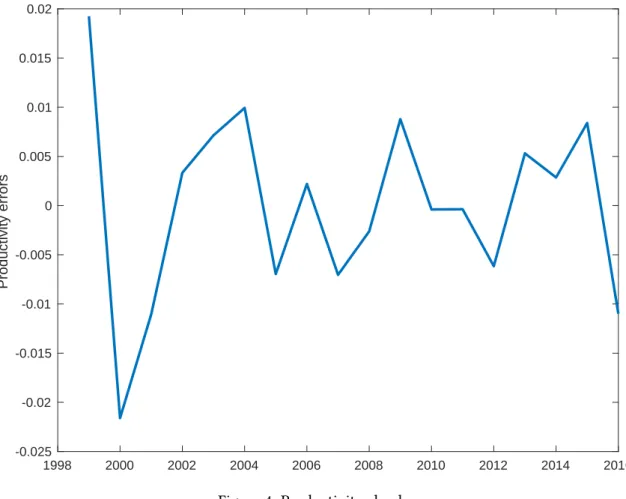
Finally, we calculate the exogenous shockstas the prediction errors of the (logged) non- linear least squares fit. Figure 4 plots the results.
4.3.2 The interest premium
We use EMBI spreads for Hungary to fit the interest premium process defined by eq. (2). We esti- mate this equation directly using an AR(1) specification with an additional explanatory variable, the NFA/GDP ratio. As for productivity, we look for a permanent change in the process, and we
1The series should be interpreted relative to a steady state of 1. We implement this empirically by also calculat- ing the TFP series for Germany, and use PPP GDP per capita in 2010 for Hungary and Germany to anchor relative productivity in Hungary in that year. This essentially means that we construct a chain-linked productivity series for Hungary at constant PPP, where German productivity in 2010 equals 1.
1998 2000 2002 2004 2006 2008 2010 2012 2014 2016 0.33
0.34 0.35 0.36 0.37 0.38 0.39 0.4 0.41 0.42
Normalized productivity
Figure 3: Transition productivity
model this change as an increase in the debt elasticity of the interest premiumψ. Empirically, we interact NFA/GDP with a dummy variable that equals one starting in 2009, the first full year of the global financial crisis.
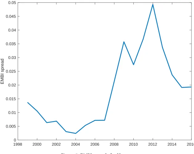
Figure 5 plots the evolution of the EMBI spread in Hungary. It is clear that there is a large and persistent increase during the global financial crisis. The precise timing is not clear from the chart, since the spread started rising in 2008. We experimented with various cutoff dates, and chose 2009 as the best fit. The estimated debt elasticities are given asψ1 = 0.0054for 1999-2008, andψ2 = 0.0279for 2009-2016. We also estimate an autoregressive coefficient ofρr = 0.49.
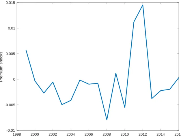
We calculate the exogenous premium shocks as the residuals to the estimated equation. The results are shown on Figure 6. There are two things worth mentioning. First, we identify mostly negative shocks until 2008. This is consistent with conventional wisdom, which considers the pre-crisis years to be a time of easy borrowing. Second, the empirical model needs a large - but temporary - shock in 2012 to explain the increase in the interest premium when the NFA/GDP ratio was already increasing. Since 2012 was the peak of the Euro crisis, which was exogenous
1998 2000 2002 2004 2006 2008 2010 2012 2014 2016 -0.025
-0.02 -0.015 -0.01 -0.005 0 0.005 0.01 0.015 0.02
Productivity errors
Figure 4: Productivity shocks
to the Hungarian economy, a large positive premium shock is precisely what we would expect.
5 Results
In this section we use the two identified processes - productivity and the interest premium - to see how well our model can match the growth experience of Hungary in the 1999-2016 pe- riod. Afterwards, we run counterfactuals when we shut off one of the two structural changes we estimated. First, we simulate the effect of the productivity slowdown only, and second, we sim- ulate the effect of the risk premium increase. Essentially, we want to run a horse-race between these two important drivers of the Hungarian growth experience after 2005, and see which one contributed more to the observed dynamics of indebtedness, investment and GDP.
5.1 Solution method
We start by simulating the model given the calibrated parameters, the estimated coefficients from the productivity and interest premium processes, and the identified i.i.d. shockst and
1998 2000 2002 2004 2006 2008 2010 2012 2014 2016 0
0.005 0.01 0.015 0.02 0.025 0.03 0.035 0.04 0.045 0.05
EMBI spread
Figure 5: EMBI spreads for Hungary
rt. We start the model from the actual initial conditions in 1999, and simulate the economy by assuming that it converges to the unique deterministic steady state in the very long run. Since the initial conditions are very far from the eventual steady state, we do not log-linearize the model equations. Instead, we apply the so-called extended path method described in Gagnon (1990).
The method is an extension of the perfect foresight solution technique that uses the New- ton method. It simplifies the original stochastic, non-linear environment by assuming certainty equivalence. At any given timet, agents are given initial conditions for endogenous and ex- ogenous state variables, and they observe the two exogenous shocks (productivity and interest premium). They assume that the economy will not be hit by new shocks in the future, which is equivalent to assume certainty equivalence. Agents therefore choose plans - and in particu- lar, pick timetchoice variables - by solving a perfect foresight problem. The realized choices for investmentit, the capital stockktand asset levelbtare stored and become initial conditions for periodt+ 1 decisions. When the next period arrives, agents again realize the new shocks (t, rt)and again solve a perfect foresight problem generating endogenous variables fort+ 1.
1998 2000 2002 2004 2006 2008 2010 2012 2014 2016 -0.01
-0.005 0 0.005 0.01 0.015
Premium shocks
Figure 6: Interest premium shocks
The simulation continues until we reach 2016, the last period for which we have data.
The perfect foresight simulations are carried out in DYNARE. The deterministic solution method assumes that the economy converges to the steady state in finite time, and solves a (large) system of equations using a version of the Newton method. Given the unique deter- ministic convergence path, we can make the approximation error arbitrarily small by choosing a distant enough point when the terminal conditions (being in the steady state) are imposed.
We selectT = 400as the length of each deterministic simulation, by which time the system is indistinguishable from the steady state.
Note that at each time period we only store the first element of the solution vector, since the next period brings new shocks and therefore requires a new simulation. We assemble the stochastic solution by combining these elements into a single time series. Also note that while we impose certainty equivalence, the deterministic non-linear features of the model are fully retained. Since we are interested in the convergence of a country far from its long-run steady state, and because the error from ignoring precautionary saving tends to be small in this class
of models, we believe that our solution method is the best compromise between speed, accuracy and tractability.2
The model has three endogenous and two exogenous state variables. As initial conditions we choose actual 1999 values, which are given by:
K1999
Y1999 = 4.788 I1999
Y1999
= 0.252 B1999
Y1999 =−0.689 A0 = 0.331 υ1999 = 0.0137.
In each subsequent period we use the previous period’s choices as initial conditions. Importantly, while we have structural breaks in 2006 and 2009, we use the model to create the appropriate initial conditions for capital, investment, the net foreign asset position, transition productivity, and the interest premium. In other words, we rely on the model to endogenously update the state variables in response to the unexpected, permanent changes to the productivity process and to the interest premium function.
5.2 Growth simulation
We now present results from the model simulations. To recap, agents face unexpected, i.i.d.
productivity and risk premium shocks. In addition we introduce two unexpected, permanent changes over time. First, the productivity convergence process - captured by the deterministic dynamics of the variableAt- slows drown dramatically after 2005. Second, the debt elasticity of the external interest premium increases significantly after 2008. The former change is specific to the Hungarian economy, while the second is the local effect of the global financial crisis. We solve and simulate the model by the extended path method detailed in the previous section.
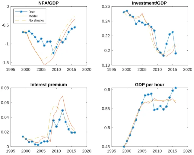
In addition to the stochastic model, we also run a deterministic simulation, where the only
2DYNARE can be downloaded from www.dynare.org. Although the software contains an explicit command for extended path simulations, we chose to program the subsequent iterations using only the deterministic solver. Since we only have 17 iterations between 1999-2016 (we use 1999 only for initial conditions), and each deterministic step takes much less than a second even with our chosen planning horizon of 400 periods, the whole procedure is very fast.
shocks are the two unexpected, permanent changes. In other words, we simply shut down the i.i.d. period shocks. We do this to see how much the long-run dynamics are influenced by the short-run shocks. Also, in the next section when we present counterfactuals, it is simpler to work with the deterministic version of the model.
1995 2000 2005 2010 2015 2020 -1.5
-1 -0.5
0 NFA/GDP
Data Model No shocks
1995 2000 2005 2010 2015 2020 0.18
0.2 0.22 0.24
0.26 Investment/GDP
1995 2000 2005 2010 2015 2020 0
0.02 0.04 0.06
0.08 Interest premium
1995 2000 2005 2010 2015 2020 0.45
0.5 0.55 0.6
GDP per hour
Figure 7: Simulating the Hungarian economy
Figure 7 presents the results. We plot four time series: the NFA/GDP ratio, the investment GDP ratio, the interest premium, and GDP pre capita normalized by trend growthXt. In each case, we plot simulations from the full stochastic model (“Model”), the deterministic model with the two unexpected permanent changes (“No shocks”), and the data (“Data”). As explained earlier, the interest premium is measured by the EMBI spread in the data.
Before we go into details, it is crucial to emphasize that we the two main driving forces - productivity and the interest premium - are taken directly from the data, and are not calibrated to match aggregate properties of the data. This is particularly true for the interest premium function, which we assume is observable. The debt elasticities are direct estimates from the EMBI
data, and are not targeted to match the forward-looking choices for investment and debt. While productivity is measured by the Solow residual, the model misses some potentially important factors such as endogenous labor supply and capacity utilization.
Given these, the model does a remarkably good job replicating key features of the Hungar- ian growth experience. In particular, both the evolution of the net foreign asset position and the investment rate are matched very well, although the model over-predicts the extent of in- debtedness before the crisis. It does, however, do a very good job in capturing the balance sheet adjustment after 2008. We also capture the evolution of the interest premium well, which is not automatic given that we let the model predict the NFA position and not use the actual value from the data in the interest premium function.
There are naturally discrepancies, which can easily be explained by factors missing from the model. One such issue is the investment boom in 2014-2015. In a related paper (Baksa- Kónya, 2017) we show that European Union structural funds have a very strong impact on the aggregate investment rate post-2010, and in these two years EU fund inflows were particularly large. Another issue is the evolution of GDP per capita in the second half of the sample. While we capture the slowdown well on average, GDP growth was stronger just before the crisis, weaker during the crisis years, and stronger again in the last two years of the sample period. The first episode is due to a sharp rise in capacity utilization, and also to a slower than predicted actual drop in capital accumulation. During the crisis, both capacity utilization and employment fell.
Finally, starting from 2013 employment has increased significantly in Hungary, at least partly driven by policy changes that encourage labor force participation.
Both capacity utilization and labor supply could be included into the model, but especially the latter presents some modeling challenges. The standard model of labor-leisure choice, which relies on an elastic labor supply, is generally considered to be a weakness of the neoclassical growth model to deliver realistic responses to productivity and interest premium shocks (Baksa and Kónya, 2017). In particular, it turns out to be difficult to have endogenous labor supply that is consistent with both the business cycle and the convergence behavior of employment. To sum up, we opted for the simplest and most robust specification that captures the long and medium term trends, instead of matching short-run fluctuations with many shocks and mechanisms.
Finally, let us briefly discuss the impact of the stochastic i.i.d. shocks on Hungarian growth.
The main difference is in the behavior of the interest premium and its impact on the net foreign
asset position. Recall that before the crisis the premium shock is mostly negative, leading to a somewhat higher level of debt than in the deterministic case. Also, in the absence of favorable temporary premium shocks, the balance sheet adjustment would have started a year or two earlier. Overall, however, the differences are modest, and the deterministic model is not notably worse in capturing the long-run dynamics of the Hungarian economy then the stochastic one.
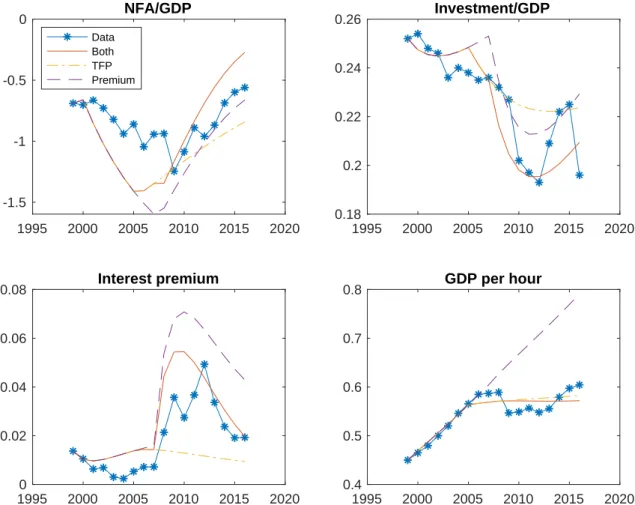
5.3 Counterfactuals
Now we turn to our main question, which is to isolate the effects of the productivity growth slow- down and the increase in the interest premium. To do this, we run two additional simulations.
First, we focus on the productivity slowdown after 2005, and assume that the debt elasticity of the interest premium does not increase in 2009. This does not necessarily assume away the global financial crisis, since it may have contributed to the prolonged slow growth of productivity in Hungary. We ignore only the direct effect of the crisis on borrowing costs. Second, mirroring the first counterfactual, we shut off the productivity channel and focus only on the financial shock.
We present results from the deterministic case and ignore period shocks, since these were identified from the observed behavior of productivity and the interest rate. In the absence of the permanent shocks, it is unlikely that the stochastic components would have behaved exactly the same way. Also, as we have shown above, the deterministic model is not significantly worth in explaining medium term dynamics in Hungary.
Figure 8 presents the results. In terms of economic growth, the dominant force is clearly the productivity slowdown. The premium increase has only a marginal impact on the evolution of GDP per capita after 2005. Our model is very simple and does not have financial accelerator type effects. It is nevertheless very unlikely that such effects would depress GDP growth for a decade.
The main reason for the lackluster growth performance of the Hungarian economy over the last decade is the low growth of productivity.
The premium increase associated with the financial crisis, however, had a significant impact on investment. Neither change alone can explain the deep drop in investment, but the premium increase seems to be the more important component. As the first panel shows, the interest pre- mium increase is responsible for the speed of the balance sheet adjustment, and one way to de- crease indebtedness is to cut back investment. Overall, while the main driver of growth seems to have been productivity, the premium increase is responsible for the bigger part of the investment
1995 2000 2005 2010 2015 2020 -1.5
-1 -0.5
0 NFA/GDP
Data Both TFP Premium
1995 2000 2005 2010 2015 2020 0.18
0.2 0.22 0.24
0.26 Investment/GDP
1995 2000 2005 2010 2015 2020 0
0.02 0.04 0.06
0.08 Interest premium
1995 2000 2005 2010 2015 2020 0.4
0.5 0.6 0.7
0.8 GDP per hour
Figure 8: Productivity or finance: counterfactual simulations decline.
6 Conclusion
In this paper we have shown that the neoclassical growth model provided a good framework to analyze the uneven convergence behavior of the Hungarian economy. In particular, empiri- cally identified processes for productivity and the external interest premium are sufficient driving forces to explain the medium-term growth performance of Hungary before and after the global financial crisis. Overall, the slowdown in TFP convergence is responsible for the sustained slug- gish growth in GDP per hour. To understand the behavior of investment and the net foreign asset position, however, interest premium developments are crucial.
The model simplifies along two important dimensions. First, it abstract away from the pub- lic sector and the role of EU funds that are important to understand short-run fluctuations in investment behavior. Second, we do not endogenize labor supply, which would be useful to ex-
plain GDP per capita growth (as opposed to GDP per hours). Both extensions present numerous challenges that we plan to take up in future work.
References
[1] Aguiar, M. and G. Gopinath (2007). “Emerging Market Business Cycles: The Cycle Is the Trend.”Journal of Political Economy,115: 69–102.
[2] Baksa, D. and I. Kónya (2017). “Interest premium and economic growth: the case of CEE.”
NBP Working Papers 266, Narodowy Bank Polski, Economic Research Department.
[3] Basu, S. (1996). „Procyclical Productivity: Increasing Returns or Cyclical Utilization?” The Quarterly Journal of Economics,111: 719–751.
[4] Benczúr, P. and I. Kónya (2016). “Interest premium, sudden stop, and adjustment in a small open economy.”Eastern European Economics,54: 271-295.
[5] Caselli, F. (2005). „Accounting for Cross-Country Income Differences.” InHandbook of Eco- nomic Growth,p. 679 – 741.
[6] Christiano, L., M. Eichenbaum and C. Evans (2005). “Nominal Rigidities and the Dynamic Effects of a Shock to Monetary Policy.”Journal of Political Economy,113: 1-45.
[7] Fazekas, K. and J. Varga, eds. (2015).The Hungarian Labor Market 2015, Budapest, IECERS- HAS.
[8] Gagnon, J. (1990). “Solving the Stochastic Growth Model by Deterministic Extended Path.”
Journal of Business & Economic Statistics,8: 35-36.
[9] García-Cicco, J., R. Pancrazi and M. Uribe (2010). “Real Business Cycles in Emerging Coun- tries?”American Economic Review,100: 2510–2531.
[10] Guerron-Quintana, P. (2013). “Common and idiosyncratic disturbances in developed small open economies.”Journal of International Economics,90: 33-49.
[11] Hall, R. E and C. I. Jones (1999). „Why do Some Countries Produce So Much More Output Per Worker than Others?”The Quarterly Journal of Economics,114: 83–116.
[12] Kónya, I. (2018).Economic growth in small open economies: lessons from the Visegrad coun- tries.Palgrave MacMillan.
[13] Levenko, N., K. Oja and K. Staehr (2019). “Total factor productivity growth in Central and Eastern Europe before, during and after the global financial crisis.”Post-Communist Economies,31: 137-160.
[14] Naoussi, C. and F. Tripier (2013). „Trend shocks and economic development.” Journal of Development Economics,103: 29-42.
[15] Schmitt-Grohé, S. and M. Uribe (2003). „Closing small open economy models.”Journal of International Economics,61: 163–185.
[16] Tastan, H. (2013). “Real business cycles in emerging economies: Turkish case.”Economic Modelling,34: 106-113.