1
Vertical Intra-Industry Trade and the EU Accession:
The Case of Hungarian Agri-Food Sector
Imre Ferto1* and Attila Jambor2
1 Institute of Economics, Centre for Economic and Regional Studies, Hungarian Academy of Sciences (email: ferto.imre@krtk.mta.hu) and Corvinus University of Budapest
(email: imre.ferto@uni-corvinus.hu)
2 Corvinus University of Budapest (attila.jambor@uni-corvinus.hu)
Paper prepared for presentation at the 87th Annual Conference of the Agricultural Economics Society, University of Warwick, United Kingdom
8 - 10 April 2013
Copyright 2013 by [Imre Ferto and Attila Jambor]. All rights reserved. Readers may make verbatim copies of this document for non-commercial purposes by any means, provided that this copyright notice appears on all such copies.
*Corresponding author: Imre Ferto (ferto.imre@krtk.mta.hu)
Postal address: Institute of Economics, Centre for Economic and Regional Studies, Hungarian Academy of Sciences, Budaörsi út 45, Budapest, H-1112
The authors gratefully acknowledge financial support from the Hungarian Scientific Research Fund No. 83119 “Changes and determinants of Central and Eastern European agricultural trade”.
Abstract
The aim of this paper is to examine the relationship between the factor endowment and the pattern of intra-industry trade. Our empirical analysis relates to Hungary’s intra-industry trade in agri-food products with 26 member states of the EU over the period 1999-2010.
Estimations reject the comparative advantage explanation of vertical intra-industry trade and provide partial support the prediction of Flam and Helpman model. Findings highlight that nature of factor endowments play also important role in explanation of vertical intra-industry trade. Other variables like market size and distance confirm the theoretical expectations. In addition, trade with new member states positively, whilst the EU accession ambigouosly influence the share of vertical IIT.
Keywords Vertical intra-industry trade, agri-food products, EU accession JEL codes Empirical Studies of Trade: F14
Economic Integration: F15
Agriculture in International Trade: Q17
2 1. Introduction
Last decades the intra-industry trade (IIT) became widespread phenomena with growing role in international trade (Brülhart, 2009). The formation of stronger economic ties between European countries due to the creation and expansion of the EU contributed to an increase in intra-industry trade among European countries. Last two decades Central and Eastern European countries also reoriented their trades from within former bloc states to the EU member countries, and the share of IIT with the EU also increased.
Theoretical literature on the IIT emphasises the role of distinction between horizontal and vertical IIT. In the case of horizontal product differentiation the usual conclusions are about the role of factor endowments and scale economies that stem from the framework of monopolistic competition. This framework, summarised in Helpman and Krugman (1985), and often referred to as the Chamberlin-Heckscher-Ohlin (C-H-O) model, allows for inter- industry specialisation in homogeneous goods and intra-industry trade in horizontally differentiated goods. This model suggests a negative relationship between differences in relative factor endowment, proxied usually by GDP per capita, and the share of IIT. However the vertical IIT models developed by Falvey (1981), Falvey and Kierzkowski (1987) and Flam and Helpman (1987) predict a positive relationship between IIT and differences in relative factor endowment. There is a growing evidence that the vertical IIT has dominant role in the total IIT (e.g. Fontagné et al. 2006) highlighting the importance of its theoretical models for the empirical analysis.
However significant part of the studies still have focused on industrial products in a C-H-O framework, and agri-food sectors are usually neglected in empirical works. The main reason is probably that agricultural markets are still usually assumed by perfect competition. But, recent studies support the view that agricultural markets can be characterised by imperfect competition (Sexton, 2013) and IIT has increasing role in agricultural trade for both developed and developing countries (e.g. Leitao 2011, Rasekhi and Shojaee 2012, Wang 2009, Varma 2012).
Hungary became a member of the European Union (EU) in 2004. We focus on the intra- industry nature of agri-food flows between Hungary and the EU after 1999, a period when the EU accession should have had a positive effect on this type of trade. More specifically, the aim of this paper is to examine the impact of EU accession on the vertical IIT.
The next section presents the theoretical foundation of the empirical model. In section 3 empirical evidence on the IIT in the agri-food sector and New Member States. Section 4 outlines the separation of horizontally and vertically differentiated products and the three approaches to measuring IIT, and these approaches are applied to our data set in section 5.
The theoretical basis for investigation of the country-specific determinants of IIT is outlined in section 6, and the results of the regression analysis are presented in section 7. Section 8 contains a summary and some conclusions.
2. Theoretical framework
The theoretical models for vertical IIT developed by Falvey (1981), Falvey and Kierzkowski (1987) and Flam and Helpman (1987), overcome the traditional indetermination of the direction of IIT, and they allow us to establish the pattern of varieties that are produced each country. Falvey (1981) assumes a perfectly competitive market with two countries, two goods
3
(a homogeneous product and a differentiated one) and two factors (labour and capital). He introduces technological differences between countries, but only in the homogeneous product sector. In the differentiated sector it is assumed that more capital is used in producing higher quality varieties than in lower quality ones. So, the higher income, relatively capital-abundant country specialises in exporting relatively high quality varieties, while the lower income, relatively labour-abundant country specialises in exporting low quality varieties. Falvey’s model does not have an explicit demand side, but Falvey and Kierzkowski (1987) elaborate this side.
On the demand side, goods are distinguished by perceived quality. Although all consumers have the same preferences, each individual demand only one variety of the differentiated product, which is determined by their income. Given that aggregate income is not equally distributed, consumers with lower incomes will demand low-quality varieties, and high- income consumers will demand the high qualities, regardless of their country of origin. Thus, it is possible establish a marginal level of income in such a way, that those consumers with higher earnings will purchase the varieties produced in the relatively capital-abundant country, while the low-income consumers will purchase the varieties produced in the relatively labour-abundant country. In this framework, intra-industry trade exists, because each variety of a differentiated good is produced in only one country, but is consumed in both countries. In a two-country world, the country which is relatively labour-abundant will tend to export the lower quality/labour intensive varieties of a differentiated good demanded abroad by low-income consumers and will tend to import the higher quality/capital intensive varieties demanded by high-income consumers in that country. Thus, IIT will be greater, the greater differences in the relative factor endowments (which correspond to per-capita income differences in the context of the model) between two countries. The model also suggests that vertical IIT is positively correlated with differences in the pattern of income distribution between partner countries.
A similar model of IIT in vertically differentiated products of Flam and Helpman (1987), in which North-South trade is determined by differences in technology, income and income distribution. The results of this model are very similar to those in Falvey and Kierzkovski (1987). In the model of Flam and Helpman there are two countries: a home country (North) and a foreign country (South), one factor (labour) and two goods. One of the goods is homogeneous and perfectly divisible, while other good is quality differentiated and indivisible. Both countries have the same unit labour requirements for producing the homogeneous good. Labour input per unit of output of the quality differentiated products differs between countries, where quality is a positive function of the labour input. The home country has an absolute advantage in production of all qualities, whilst the foreign country may have a comparative advantage in low quality variety. Note, that the source of quality differentiation is not the amount of capital used in producing the good, like in the Falvey and Kierzkowski (1987) model, but the technology used.
Demand for varieties stems from variation in income across consumers, who buy a specific quality reflecting their preferences and income constraint. Consumers with higher effective labour endowments (implying higher income) demand the higher quality indivisible good.
Therefore, the home country specialises completely in the differentiated good of high quality, whilst the foreign country exports the homogeneous good and the differentiated good of low quality. Assuming an overlap in income distribution, IIT appears. The model predicts that higher bilateral differences in factor endowment lead to a higher share of IIT.
4 3. Empirical evidence
Although the importance of IIT is already well documented in agri-food sectors in the late nineties (Fertő, 2005), last decade research remained still limited on the determinants of agri- food IIT. Wang (2009) investigated the IIT for China’s agricultural products between 1996 and 2005 showing a relatively low level of IIT with continuously increasing trend. Varma (2012) analysed the extent of intra-industry trade in India’s agricultural trade highlighting a mild tendency for IIT to increase during the period of 2000–2008. Fertő (2007) analysed Hungarian intra-industry agri-food trade patterns with the EU15 and confirmed that determinants for horizontal and vertical IIT differed. Horizontal intra-industry trade was negatively associated with differences in per capita income, average GDP, distance and distribution of income, while income and distance are positively related to VIIT. Leitao and Faustino (2008) investigated the determinants of intra-industry trade (IIT) in the Portuguese food processing sector and found that IIT was positively influenced by GDP per capita differences and energy consumption, while it was negatively related to physical endowments, relative size effects and geographical distance. Leitao (2011) focused on the determinants of United State’s agricultural IIT and showed that it was positively influenced by average GDP, FDI and trade imbalance, while it had a negative relationship with differences in per capita GDP. Rasekhi and Shojaee (2012) investigated the country specific determinants of vertical and total intra-industry trade between Iran and its main trading partners and proved that vertical IIT was positively influenced by land endowments, but negatively affected by the size of trading partners.
In short, studies highlighted the increasing role of intra-industry trade in agri-food trade for some developed and developing countries. In addition, in line of recent empirical evidences papers confirm that horizontal and vertical IIT are influenced by different factors.
Second group of the literature concentrates on the IIT in the New Member States (NMS).
Caetano and Galego (2007) investigated the determinants of intra-industry trade within an enlarged Europe and also found that determinants of horizontal and vertical IIT differed, although both had a statistically significant relationship with a country’s size and foreign direct investment. According to their results, country size, income per capita differences and geographic distance were found to be important factors for IIT, especially for horizontal IIT.
Jensen and Lüthje (2009) analysed driving forces of VIIT in Europe and identified production size, geographical proximity, average income per capita and income distribution overlap as the major ones. It was proven that countries characterized by being on a high economic level and by being large economies had a higher bilateral VIIT with each other than with other countries. Furthermore, countries with large income distribution overlap tended to have a large VIIT, while countries far from each other had lower VIIT than countries close to each other.
Gabrisch (2009) investigated the VIIT between old and new member states of the EU and found that country-pair fixed effects to be of high relevance for explaining vertical intra- industry trade. His results suggest that technology differences were positively, while differences in factor endowment were negatively correlated with vertical intra-industry trade.
Moreover, changing bilateral differences in personal income distribution during the transition of NMS found to be contributed to changes in vertical intra-industry trade.
Černoša (2009) tests the industry-specific hypothesis for Slovenia before the EU accession.
He found that vertical IIT is predominant within total IIT. The results provide strong support
5
for the effects of industry-specific determinants of vertical IIT. Manual labor intensity in production is a comparative advantage, whereas capital intensity in production is a disadvantage.
Fainštein and Netšunajev (2011) analysed intra-industry trade dynamics for Estonia, Latvia, and Lithuania in 1999-2007. Their results show that shares of IIT have increased within the period, with vertical IIT dominating. Shares of total vertical and horizontal IIT have grown since 2004, the year of accession to the European Union. They find market size, distance and human capital to be important in the Baltic states for IIT in general and for horizontal IIT in particular.
Ambroziak (2012) investigated the relationship between FDI and IIT in the Visegrad countries and found that FDI stimulated not only VIIT in the region but also HIIT. He found that differences in country size and income were positively related to IIT as is FDI, while distance and IIT showed a negative relationship.
In sum, research on the IIT in NMS confirms the dominance of vertical IIT over horizontal IIT. Results also imply the distinction between horizontal and vertical IIT play important role to explain the drivers of IIT.
4. Measuring vertical and horizontal intra-industry trade
The basis for the various measures of IIT used in the present study is the Grubel–Lloyd (GL) index (Grubel and Lloyd, 1975), which is expressed formally as follows:
) 1 (
i i
i i
i X M
M GL X
(1)
where Xi and Mi are the value of exports and imports of product category i in a particular country. The GL index varies between 0 (complete inter-industry trade) and 1 (complete intra- industry trade) and can be aggregated to level of countries and industries as follows:
n
i GLiwi
GL 1 where
n
i i i
i i
i X M
M w X
1( )
)
( (2)
where wi denotes the share of industry i in total trade.
Literature suggests several options to disentangle the horizontal and vertical IIT. Greenaway et al. (1995) developed the following approach, a product is horizontally differentiated if the unit value of export compared to the unit value of import lies within a 15% range, and otherwise they define vertically differentiated products. Formally, this is expressed for bilateral trade of horizontally differentiated products as follows:
1
1 M
i X i
UV
UV (3)
where UV means unit values, X and M means exports and imports for goods i and ά=0.15.
Furthermore, Greenaway et al. (1994) added that results coming from the selection of the 15%
range do not change significantly when the spread is widened to 25%. Blanes and Martín (2000) emphasise the distinction between high and low VIIT. They define low VIIT when the relative unit value of a good is below the limit of 0.85, while unit value above 1.15 indicates high VIIT.
6
Based on the logic above, the GHM index comes formally as follows:
j
k j k j j
p k j p
k j p
k j p
k j p
k X M
M X
M X
GHM
, ,
, ,
, ,
(4)
where X and M denote export and import, respectively, while p distinguishes horizontal or vertical intra-industry trade, j is for the number of product groups and k is for the number of trading partners (j, k = 1, ... n).
Fontagné and Freudenberg (1997) propose a different method in the literature categorize trade flows and compute the share of each category in total trade. They defined trade to be "two- way" when the value of the minority flow represents at least 10% of the majority flow.
Formally:
% ) 10 , (
) ,
(
Mi Xi Max
Mi Xi
Min (5)
If the value of the minor flow is below 10%, trade is classified as inter-industry in nature. If the opposite is true, the FF index comes formally as:
j
k j k j j
p k j p
k j p
k X M
M X
FF
, ,
, ,
(6)
After calculating the FF index, trade flows can be classified as follows: horizontal two-way trade, vertical two-way trade and one-way trade.
According to Fontagné and Freudenberg (1997), the FF index tendentiously provides higher values compared to GL-type indices (like the GHM index) as equation 5 refers to total trade, treated before as two-way trade. The authors suggest that FF index rather complements than substitutes GL-type indices as they have measured the relative weight of different trade types in total trade. In conclusion, they found that the value of GHM index is usually between the GL and FF index.
Previous indices measure the share of intra-industry trade instead of its level. Nilsson (1997) suggests a new indicator that matched trade [i.e. the same numerator as GHM in (4)] is divided by the number of products traded, n, to yield an average level of IIT per product.
Fertő (2005) applied this logic to horizontal and vertical IIT and formally express the N index as:
p j
p k j p
k j p
k j p
k j p
k n
M X
M X
N
, ,
, ,
(7)
where the numerator equals to that of the GHM index, while n refers to the number of product groups in total trade. Nilsson (1997) argues that his measure provides a better indication of the extent and volume of IIT than GL-type indices and is more appropriate in cross-country IIT analyses.
7
We employ trade data from the Eurostat COMEXT database using the HS6 system (six digit level). Agri-food trade is defined as trade in product groups HS 1-24, resulting in 964 products using the six digit breakdown. Our analysis focuses on the period 1999-2010. In this context, the EU is defined as the member states of the EU27.
5. Hypotheses and econometric specifications
Following the theoretical and empirical research we test the following hypotheses.
H1. Difference in factor endowments between trading partners increases the share of vertical IIT in total trade.
Difference in factor endowments is a key variable when explaining vertical IIT. In the empirical literature factor endowments are usually proxied by the GDP per capita. Relative factor endowments is measured by the logarithm of absolute value of the difference in per capita GDP is used between Hungary and her trading partners (lnDGDPC), which is expected to be positively related to the share of vertical IIT. Per capita GDP is measured in PPP in current international dollars and data comes from the World Bank WDI database. However, the use of per capita GDP as a proxy for relative factor endowments is problematic. Linder (1961) already noted that inequality per capita income may serve as a proxy for differences in preferences as suggested. In addition, Hummels and Levinsohn (1995) argued that this proxy is appropriate only when the number of factors is limited to two and all goods are traded, thus they proposed income per worker as a measure of differences in factor composition and also using actual factor data on capital–labor and land–labor ratios. Interestingly, despite of these limitations of use of the GDP per capita, it became a popular and dominating proxy for factor endowments in empirical literature. However, nature of factor endowments may play also important role in specialisation in quality ranges. Thus, it is necessary to use more variables to consider various aspects of factor endowments including physical, technological and human capital. The standard solution is to employ investment in physical capital, R&D expenditures and education expenditure (e.g. Milgram-Baleix and Moro-Egido, 2010).
Note, our focus is the agri-food trade, thus we employ more agricultural related factor endowments variables. More specifically, we concentrate three traditional agricultural factors including land, labour and capital. Consequently, we measure relative agricultural factor endowments by the logarithm of absolute value of the difference in agricultural land, labour and machinery between Hungary and its trading partners (lnDLAND, lnDLAB, lnDMACH), which are expected to be positively related to the share of vertical IIT. Agricultural land is measured in million hectares, agricultural labour is measured in 1000 annual working units, while agricultural machinery is measured in euro.
H2. The growth of average economic size increases the share of vertical IIT in total trade.
The larger the international market, the larger the opportunities for production of differentiated intermediate goods and the larger the opportunities for trade in intermediate goods. The logarithm of the absolute difference in the average GDP of trading partners is used as a proxy for the average size of markets. AVGDP is measured in PPP in current international dollars and the source of data is also the World Bank WDI database. A positive sign for vertical IIT is expected.
8
H3. The more unequal income distribution in trading partners increases the share of vertical IIT in total trade.
Unequal income distribution suggests different demand patterns between trading partners and thereby the need for quality-differentiation (associated with vertical IIT) arises. This hypothesis is tested by using the logarithm of absolute value of the difference in the GINI- index between Hungary and EU27, which is expected to be positively related to the share of vertical IIT. Data for the lnDGINI variable is coming from the World Bank WDI.
H4. IIT will be greater the closer the countries are geographically.
The distance between countries well reflects transport costs. Variable lnDIST indicates the geographic distance between the reporting country and each of its trading partners by calculating the logarithm of the distance between the capital cities of trading partners in kilometres. The source of data is the CEPII database. LnDIST is expected to be negatively related to VIIT.
In addition, we test two specific hypotheses. Previous studies (Fertő and Soós 2009, and Bojnec and Fertő 2012) show that the duration of trade in both manufacturing and agri-food products differs across EU10/12 and EU15 markets: for the majority of countries the length of trade is greater in EU10/12 markets than in EU15 markets. These result reveal the hypothesis.
H5: The share of VITT differs between New and Old Member States markets.
Finally, our main interest is the impact of EU accession to the VIIT in Hungarian agri-food trade. It is generally accepted that economic integration increases VIIT.
H6: The EU accession has positive impact on the share of VIIT.
We test the model by Flam and Helpman (1987) with two baseline specifications.
lnIITijt= α0+ α1lnDGDPCijt + α2lnDAVGDPijt + α3lnDGINIijt + α4lnDISTijt + α5NMSt + α6EU
+ vij + ij (8)
lnIITijt= α0+ α1lnDLANDijt + α2lnDLABijt + α3lnDMACHijt + α4lnDAVGDPijt + α5lnDGINIijt + α6lnDISTijt + α7NMSt + α8EU + vij + ij (9) Table 1 provides an overview of the description of variables and related hypotheses.
Table 1: Description of independent variables
Variable Variable description Data source Sign
lnDGDPC The logarithm of per capita GDP absolute difference between trading partners measured in PPP in current international USD
WDI +
lnDLAND The logarithm of agricultural area absolute difference between trading partners measured in million hectares
WDI +
lnDLAB The logarithm of agricultural labour absolute difference between trading partners measured in 1000 annual working units
Eurostat +
lnDMACH The logarithm of agricultural machinery absolute difference between trading partners measured euro
FADN +
lnAVGDP The logarithm of average GDP absolute difference between WDI +
9
trading partners measured in PPP in current international USD lnDGINI The logarithm of GINI absolute difference between trading
partners measured by the GINI index
WDI +
lnDIST The logarithm of absolute difference between trading partners capital city measured in kilometres
CEPII -
NMS dummy variable: 1 if NMS, otherwise zero ?
EU dummy variable: 1 when Hungary is member of the EU, otherwise zero
+ Source: Own composition
6. The nature of intra-industry trade
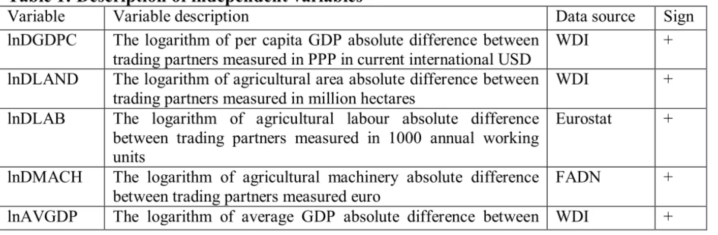
Using the methods outlined above, we compute measures of IIT in horizontally and vertically differentiated agri-food products between Hungary and 26 member states of the EU, for the period 1999 to 2010, using Eurostat data. From the average measures of GHM, FF and N over the period, Hungary’s IIT in agri-food products with its EU partners was increasing (Figure 1). The three indices yield a relatively good consistency for ranking countries according to the share of horizontal and vertical IIT, the nine possible pairings show a high level of correlation (>0.85).
Figure 1: Development of IIT between Hungary and EU-26 using different measures
Source: Own calculations based on the Eurostat database
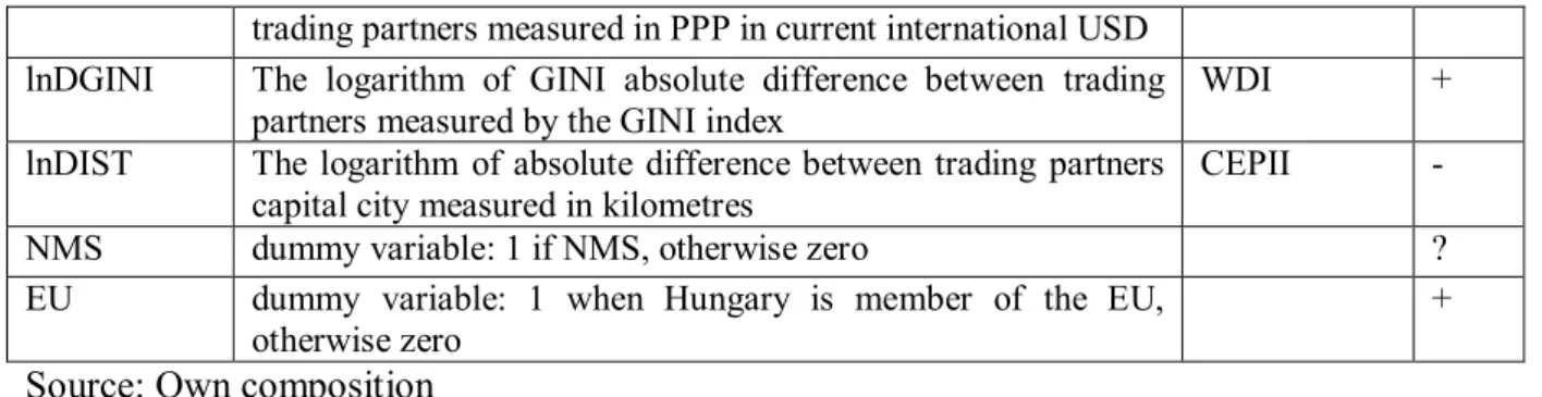
Furthermore, there is evidence of IIT, mainly of a vertical nature, suggesting the exchange of products of different quality (Figure 2). The dominance of vertical over horizontal type trade accords with the general findings of recent empirical literature. Simple t tests suggest that Hungary specialises in larger shares of lower than higher qualities of agri-food products irrespective to various IIT indices. Interestingly, we find some evidence on the difference between two market segments of the EU. Kruskal-Wallis tests reveal that the share of high and low VIIT significantly higher in the OMS than in the NMS, while the share of HIIT does not differ across market segments. In the rest of this paper, we abstract from the horizontal term of the various indices of IIT, and focus only on vertical IIT. This means that we keep about 84 per cent of Hungarian IIT with the EU countries.
0 10000 20000 30000 40000 50000 60000 70000
0 0,05 0,1 0,15 0,2 0,25
1999 2000 2001 2002 2003 2004 2005 2006 2007 2008 2009 2010
GHM FF N
10 Figure 2: Types of IIT by market segments
Source: Own calculations based on the Eurostat database 7. Regression results
Before estimating the panel regression models, the main model variables are pre-tested for unit root tests. A number of panel unit root tests are available. Considering the well known low power properties of unit root tests, in this paper we employ a battery of unit root tests:
Levin, Lin and Chu (2002) method (common unit root process), Im, Pesaran and Shin (2003) method (assuming individual unit root processes), ADF-Chi square, and PP-Chi square. Table 2 presents the results of four different panel unit root tests (Levin, Lin and Chu; Im, Pesaran and Shin; ADF-Fisher Chi square, PP-Fisher Chi square), with different deterministic specifications (with constant, and with constant and trend). Mixed results were obtained. The most important model variables such as the bilateral trade flows and R&D expenditures in countries i and j do not have unit roots, i.e. are stationary, with individual effects and individual trend specifications. The panel unit root null hypothesis is also rejected with constant only deterministic specification for Levin, Lin and Chu and PP-Fisher Chi-square tests. Other variables such as GDP and GDPCAP are more ambiguous in terms of unit root in a panel context. We may conclude that with the individual effects specification both variables of the panel dataset are stationary, while the majority of test results accept the panel unit root null hypothesis.
Table 2: Panel unit root tests
GHM FF N lnDGDPC lnAVGDP lnDLAND lnDLAB lnDMACH
Levin, Lin & Chu t* 0.000 0.013 0.735 0.012 0.000 1.000 0.000 1.000 Im, Pesaran and Shin W-
stat
0.000 0.295 0.842 0.809 0.000 1.000 0.664 0.993
ADF - Fisher Chi-square 0.000 0.020 0.042 0.887 0.001 1.000 0.933 0.996 PP - Fisher Chi-square 0.000 0.000 0.000 0.987 0.000 1.000 0.632 1.000 with trend
Levin, Lin & Chu t* 0.000 0.000 0.000 0.000 1.000 1.000 0.005 1.000
Breitung t-stat 0.998 0.012 1.000 0.999 1.000 1.000 0.640 1.000
Im, Pesaran and Shin W- stat
0.000 0.000 0.000 0.221 1.000 1.000 0.193 1.000
0%
10%
20%
30%
40%
50%
60%
70%
80%
90%
100%
GHM FF N GHM FF N GHM FF N
OMS NMS EU27
VLIIT VHIIT HIIT
11
ADF - Fisher Chi-square 0.000 0.000 0.000 0.141 1.000 1.000 0.354 1.000 PP - Fisher Chi-square 0.000 0.000 0.000 0.968 1.000 0.991 0.999 1.000
Source: Own estimations
To ensure that both variables are stationary I(0) and not integrated of a higher order, we apply unit root tests on first differences of all variables. All tests (not shown here) reject the unit root null hypothesis for the first differences. In sum, we may conclude that panel is likely stationary.
We apply several estimation techniques to equation (8-9) in order to ensure the robustness of the results. Due to time invariant variables including distance, EU, NMS we preclude the fixed effect panel models. However, there are some issues that we have to be addressed when are estimated such panel models. First, heteroskedasticity may occur because trade between two smaller countries or between a smaller and larger country is probably more volatile than trade between two larger countries. The panel dataset is also subject to the existence of autocorrelation. Contemporaneous correlation across panels may occur because exporting to one country can take place as an alternative to exporting to another country. Similarly, adjacent exporter(s)’/importer(s)’ time specific shocks result in larger correlated error terms of their trade with their partners. Preliminary analysis (likelihood ratio tests, Wooldridge and Pesaran tests) confirms the presence of heteroscedasticity, autocorrelation and cross-sectional dependence. Because our analysed period is shorter than cross sectional unit, to deal with issues of contemporaneous correlation the panel corrected standard error model (PCSE) is applied which controls for heteroskedasticity and the AR(1) type of autocorrelation and contemporaneous correlation across panels (Beck and Katz, 1995, 1996).
7.1. Static panel models
Empirical research faces some difficulties when interpreting results on the relationships between factor endowments variables including per capita GDP and vertical IIT. It is usually assumed that differences in factor endowments (per capita GDP) increase the exchange of different varieties, whatever the type of vertical product differentiation of the well-endowed country and poorly-endowed country. However, distinguishing the low and high quality components of vertical IIT implies that differences in factor endowments between trading partners should respond in the opposite direction. The theory suggests that the better endowed country should improve its comparative advantage only in the high quality varieties. Thus we need to modify dependent variable taking into account this quality difference. Following Fertő (2005) the dependent variable is low vertical IIT when Hungary exports to a higher per capita GDP country (above the EU average) and a high vertical IIT when Hungary exports to a lower per capita GDP country (below the EU average).
The results are quite similar for the three dependent variables. The lnDGDPC variable has the unexpected sign but it is insignificant for FF and N specifications (Table 3). Our findings differ to Rasekhi and Shojaee (2012) who find positive relationship between vertical IIT and GDP per capita differences. Similarly to others studies on manufacturing sectors our results do not support comparative advantage explanation of vertical IIT (Milgram-Baleix and Moro- Egido 2010).
Contrary to Fertő (2005) and Rasekhi and Shojaee (2012) the sign of factor lnDLAND variables is unexpectedly negative and significant for all specifications. The other two factor endowment variables lnDLAB and lnDMACH have positive sign, but they are significant jointly only for the N model. These findings reveal that nature of factor endowments is
12
important for vertical IIT. In line with previous studies for total trade (e.g. Blanes and Martin 2000, Mora 2002, Jensen and Lüthje 2009, Milgram-Baleix and Moro-Egido 2010) we find that differences in human and/or technological capital have rather positive impact on vertical IIT than physical capital differences.
Table 3: Determinants of vertical IIT in the agri-food sector (PCSE models)
GHM FF N
lnDGDPC -0.0064*** -0.0130 -4.8e+02
lnDLAND -0.0053** -0.0273*** -5.0e+03***
lnDLAB 0.0044*** 0.0043 1.3e+03**
lnDMACH 0.0001 0.0062*** 514.7944*
lnAVGDP 0.0089*** 0.0098*** 0.0203*** 0.0293*** 5.5e+03*** 7.7e+03***
lnDGINI -0.0002 -0.0002 0.0001 0.0008 -3.8e+02 -1.7e+02 lnDIST -0.0155*** -0.0203*** -0.0575*** -0.0539*** -8.0e+03** -7.9e+03**
NMS 0.0183*** 0.0239*** 0.0251 0.0779*** 1.3e+04*** 1.5e+04***
EU 0.0043 0.0027 0.0205 -0.0082 6.4e+03** 2.9e+03*
constant -0.0675 -0.1378 -0.0011 -0.4181* -9.0e+04* -1.6e+05***
N 312 312 312 312 312 312
R2 0.5618 0.5404 0.4119 0.4080 0.4768 0.5612
Source: Own estimations
Note: N: number of observations. ***/**/*: statistically significant, respectively at the 1%, 5%, and 10% levels.
The coefficients of lnAVGDP are positive and significant for all specifications confirming hypothesis 2. The income distribution overlap variables are insignificant with unexpected signs for all specifications. Distance variables have expected signs and are significant for all specifications supporting hypothesis 4. The NMS variable positively influences the share of VIIT for all specifications except baseline FF model. This implies that agrifood trade with NMS has positive impact on the VIIT. The EU accession has positive effect on VIIT only for N models, while it is not significant for other specifications.
7.2. Dynamic panel models
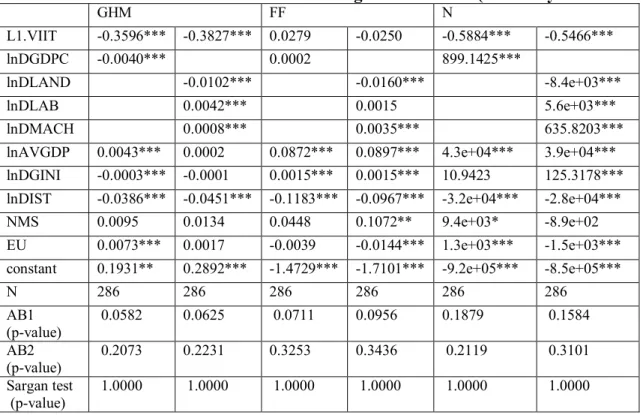
Faustino and Leitao (2007) suggest to use of dynamic panel framework to solve serial correlation, heteroskedasticity and endogeneity of some explanatory variables. In addition to PCSE approach thus we employ the generalized method of moments (GMM) estimator developed by Arellano and Bover (1995) and Blundell and Bond (1998), also referred to as GMM-system estimator. Windmeijer (2005) proposes a finite sample correction that provides more accurate estimates of the variance of the two-step GMM estimator (GMM-SYS). As the t-tests based on these corrected standard errors are found to be more reliable, the paper estimates the coefficients using the finite sample correction.
Table 4 reports results on determinants of VIIT using GMM-system estimator. The models present consistent estimates, with no serial correlation (AB1, AB2 statistics). The specification Sargan test show that there are no problems with the validity of instruments used. The GMM system estimator is consistent if there is no second-order serial correlation in
13
the residuals (AB2 statistics). The dynamic panel data are valid. We used the criterion of Windmeijer (2005) to small sample correction.
Dynamic models provide mainly similar results. Suprisingly, lagged VIIT variables are negative and significant for GHM and N models contrary to Faustino, and Leitão (2007) and Leitão (2011). Similarly to PCSE model DGPDC has negative and significant impact on the VIIT for GHM approach. Interestingly, DGDPC significantly positively influences the VIIT confirming hypothesis 1 for N model. GMM system estimators report the same results for factor endowment lnAVGDP and distance, except lnDMACH variables for GHM approach.
In the dynamic setting NMS variable remains positive and significant only two of six models.
The estimations on the impact of the EU accession are rather contradictiory. We have two-two negative and positive and significant coefficients depending on various specifications.
Table 4: Determinants of vertical IIT in the agri-food sectors (GMM-Systems models)
GHM FF N
L1.VIIT -0.3596*** -0.3827*** 0.0279 -0.0250 -0.5884*** -0.5466***
lnDGDPC -0.0040*** 0.0002 899.1425***
lnDLAND -0.0102*** -0.0160*** -8.4e+03***
lnDLAB 0.0042*** 0.0015 5.6e+03***
lnDMACH 0.0008*** 0.0035*** 635.8203***
lnAVGDP 0.0043*** 0.0002 0.0872*** 0.0897*** 4.3e+04*** 3.9e+04***
lnDGINI -0.0003*** -0.0001 0.0015*** 0.0015*** 10.9423 125.3178***
lnDIST -0.0386*** -0.0451*** -0.1183*** -0.0967*** -3.2e+04*** -2.8e+04***
NMS 0.0095 0.0134 0.0448 0.1072** 9.4e+03* -8.9e+02 EU 0.0073*** 0.0017 -0.0039 -0.0144*** 1.3e+03*** -1.5e+03***
constant 0.1931** 0.2892*** -1.4729*** -1.7101*** -9.2e+05*** -8.5e+05***
N 286 286 286 286 286 286
AB1 (p-value)
0.0582 0.0625 0.0711 0.0956 0.1879 0.1584 AB2
(p-value)
0.2073 0.2231 0.3253 0.3436 0.2119 0.3101 Sargan test
(p-value)
1.0000 1.0000 1.0000 1.0000 1.0000 1.0000
Source: Own estimations
Note: N: number of observations. ***/**/*: statistically significant, respectively at the 1%, 5%, and 10% levels. AB1 AB2 are tests for first-order and second-order autocorrelation 8. Summary and conclusions
In this paper, we use a vertically differentiated model of the Flam and Helpman type to investigate the relationship between factor endowment and vertical IIT in agri-food products between Hungary and its EU trading partners. Our results show, for Hungary, that horizontal IIT in agri-food products is low, but that vertical type trade is more prevalent, though still less important than inter-industry trade.
We have shown that the study relationship between vertical IIT and factor endowments displays some problems of interpretation. Therefore, we propose an alternative approach based on taking into account that a particular country exports to a low- or high income country. Moreover, in line with recent studies we introduce direct agricultural related factor endowment measures rather than per capita GDP. The results obtained here reject the
14
comparative advantage explanation of vertical IIT. Our findings provide more support to neo- factor explanation of vertical IIT. In addition, trade with new member states has positive impact, whilst the EU accession ambigouosly influence the share of vertical IIT.
The measure of IIT is subject to various criticism, thus results may be biased using different IIT indices. Our results reveal suprisingly robust results accross various measurement of ITT.
Similarly, static and dynamic model estimations are not differ considerably as we a priori expected.
References
Ambroziak, L. 2012. FDI and intra-industry trade: theory and empirical evidence from the Visegrad Countries. International Journal of Economics and Business Research, 4(1-2): 180- 198.
Arellano, M. and Bover, O. 1995. Another look at the instrumental variable estimation of error-components models. Journal of Econometrics, 68(1): 29–51.
Beck, N. and Katz, J.N. 1995. What to Do (and Not to Do) with Time-Series Cross-Section Data. American Political Sciences Review, 89(3): 634-647.
Beck, N. and Katz, J.N. 1996. Nuisance vs. Substance: Specifying and Estimating Time- Series Cross-Section Models. Political Analysis, 6(1): 1-36.
Blanes, J.V. and Martín, C. 2000. The nature and causes of intra-industry trade: Back to the comparative advantage explanation? The case of Spain. Review of World Economics, 136(3):
423-441.
Blundell, R. and Bond, S. 1998. Initial conditions and moment restrictions in dynamic panel data models. Journal of Econometrics, 87(1): 115–143.
Bojnec, S. and Fertő, I. 2012. Does EU enlargement increase agro-food export duration? The World Economy, 35(5): 609-631.
Brülhart, M. 2009. An Account of Global Intra‐industry Trade, 1962–2006. The World Economy, 32(3): 401-459.
Caetano, J. and Galego, A. 2007. In Search for Determinants of intra-industry trade within an Enlarged Europe. South-Eastern Europe Journal of Economics, 5(2): 163-183.
Černoša, Š. 2009. Intra-Industry Trade and Industry-Specific Determinants in Slovenia:
Manual Labour as Comparative Advantage. Eastern European Economics, 47(3): 84-99.
Fainštein, G., and Netšunajev, A. 2011. Intra-Industry Trade Development in the Baltic States. Emerging Markets Finance and Trade, 47(3): 95-110.
Falvey, R. 1981. Commercial policy and intra-industry trade. Journal of International Economics, 11(4): 495–511.
Falvey, R. and Kierzkowski, H. 1987. Product Quality, Intra-Industry Trade and (Im)Perfect Competition. IN Kierzkowski, H. (eds.): Protection and Competition in International Trade.
Essays in Honor of W.M. Corden. Blackwell, Oxford, UK.
Faustino, H.C. and Leitão, N.C. 2007. Intra-industry trade: a static and dynamic panel data analysis. International Advances in Economic Research, 13(3): 313-333.
Fertő, I. 2005. Vertically Differentiated Trade and Differences in Factor Endowment: The Case of Agri‐Food Products between Hungary and the EU. Journal of Agricultural Economics, 56(1): 117-134.
Fertő, I. 2007. Intra-industry trade in horizontally and vertically differentiated agri-food products between Hungary and the EU. Acta Oeconomica, 57(2): 191-208.
Fertő, I. and Soós, K.A. 2009. Treating trade statistics inaccuracies: the case of intra-industry trade. Applied Economics Letters. 16(18): 1861-1866.
Flam, H. and Helpman, E. 1987. Vertical Product Differentiation and North-South Trade.
American Economic Review, 77(5): 810–822.
15
Fontagné, L. and Freudenberg, M. 1997. Intra-industry trade: Methodological issues reconsidered. CEPII Working Papers, 97–01.
Fontagné, L., Freudenberg, M., and Gaulier, G. 2006. A systematic decomposition of world trade into horizontal and vertical IIT. Review of World Economics, 142(3): 459–475.
Gabrisch, H. 2009. Vertical intra-industry trade, technology and income distribution: a panel data analysis of EU trade with Central-East European Countries. Acta Oeconomica, 59(1): 1- 22.
Greenaway, D., Hine, R., and Milner, C. 1994. Country-Specific Factors and the Pattern of Horizontal and Vertical Intra-Industry Trade in the UK. Weltwirtschaftliches Archiv, 130(1):
77–100.
Greenaway, D. – Hine, R.C. – Milner, C.R. 1995. Vertical and Horizontal Intra-Industry Trade: A Cross-Industry Analysis for the United Kingdom. Economic Journal, 105(11):
1505– 1518.
Grubel, H. and Lloyd, P. 1975. Intra-industry Trade The Theory and Measurement of International Trade in Differentiation Products. The Mcmillan Press, London, UK.
Helpman, E. 1987. Imperfect Competition and International Trade: Evidence from Fourteen Industrial Countries. Journal of the Japanese and International Economics, 1(1): 62–81.
Helpman, E. and Krugman, P. 1985. Market Structure and Foreign Trade. Harvester Wheatsheaf, Brighton, UK
Hummels, D. and Levinsohn, J. 1995. Monopolistic Competition and International Trade:
Reconsidering the Evidence. Quarterly Journal of Economics, 110(3): 799-836.
Im, K., Pesaran, H. and Shin, Y. 2003. Testing for unit roots in heterogeneous panels. Journal of Econometrics, 115(1): 53-74.
Jensen, L. and Lüthje, T. 2009. Driving forces of vertical intra-industry trade in Europe 1996–
2005. Review of World Economics, 145(3): 469-488.
Leitão, N.C. and Faustino, H. 2008. Intra-industry trade in the food processing sector: the Portuguese case. Journal of Global Business and Technology, 4(1): 49-58.
Leitão, N.C. 2011. Intra-industry trade in the agriculture sector: The experience of United States. African Journal of Agricultural Research, 6(1): 186-190.
Levin, A., Lin, C. and Chu, C. 2002. Unit root tests in panel data: asymptotic and finite- sample properties. Journal of Econometrics, 108(1): 1-24.
Linder, S.B. 1961. An Essay on Trade and Transformation. John Wiley, New York, USA Milgram‐Baleix, J., and Moro‐Egido, A.I. 2010. The Asymmetric Effect of Endowments on Vertical Intra‐industrial Trade. The World Economy, 33(5): 746-777.
Mora, C.D. 2002. The role of comparative advantage in trade within industries: A panel data approach for the European Union. Review of World Economics, 138(2): 291-316.
Nilsson, L. 1997. The Measurement of Intra-Industry Trade between Unequal Partners.
Weltwirtschaftliches Archiv, 133(3): 554–565.
Rasekhi, S., and Shojaee, S.S. 2012. Determinant factors of the vertical intra-industry trade in agricultural sector: a study of Iran and its main trading partners. Agricultural Economics (Zemědělská Ekonomika), 58(4): 180-190.
Sexton, R.J. 2013. Market Power, Misconceptions, and Modern Agricultural Markets.
American Journal of Agricultural Economics, 95(2): 209-219.
Varma, P. 2012. An analysis of India’s bilateral intra-industry trade in agricultural products.
International Journal of Economics and Business Research, 4(1): 83-95.
Wang, J. 2009. The analysis of intra-industry trade on agricultural products of China.
Frontiers of Economics in China, 4(1): 62-75.
Windmeijer, F. 2005. A finite sample correction for the variance of linear efficient two-step GMM estimators. Journal of Econometrics, 126(1): 25–51.