C
ORVINUSU
NIVERSITY OFB
UDAPESTZsolt Darvas, Jan Mazza, Catarina Midões
Cohesion project characteristics and regional economic growth in the European Union
http://unipub.lib.uni-corvinus.hu/6420
C
O R V I N U SE
CONOMICSW
O R K I N GP
A P E R S03/2021
Cohesion project characteristics and regional economic growth in the European Union Zsolt Darvas, Jan Mazza and Catarina Midões
12 April 2021
Abstract
We employ a novel methodology for the study of the characteristics of successful European Union cohesion projects. We first estimated ‘unexplained economic growth’ by controlling for the influence of various region-specific factors, and then analysed its relationship with about two dozen cohesion project characteristics. We found that the best-performing regions have on average projects with longer durations, more inter-regional focus, lower national co-financing, more national (as opposed to regional and local) management, higher proportions of private or non-profit participants among the beneficiaries and higher levels of funding from the Cohesion Fund. No clear patterns emerged concerning the sector of intervention.
JEL classification: C21; O47; R11; R58
Keywords: EU cohesion policy; growth determinants; regional convergence; project characteristics
Zsolt Darvas is a Senior Fellow at Bruegel, and a Senior Research Fellow at the Corvinus University of Budapest, email: zsolt.darvas@uni-corvinus.hu
Jan Mazza is a PhD in Economics student at European University Institute, Firenze, Italy, email: jan.mazza@eui.eu
Catarina Midões is an MSc in Climate Change student at Ca' Foscari University of Venice, Italy, email:midoes.catarina@gmail.com
Acknowledgements
This working paper is an extended and revised version of an original study titled
“Effectiveness of cohesion policy: learning from the project characteristics that produce the best results” done by the authors (along with Antoine Mathieu Collin) on behalf of the European Parliament’s Committee on Budgetary Control (CONT). The opinions expressed in this document are the sole responsibility of the authors and do not necessarily represent the official position of the European Parliament. The authors thank Kaare Barslev, István Kónya, several colleagues from the European Parliament and European Commission as well as seminar and conference participants at the European Parliament, Bruegel, the 2020 European Week of Regions and Cities, and the 2020 Conference of the Hungarian Economic Association for comments and suggestions.
1 Introduction
A key objective of the European Union is to strengthen regional cohesion by addressing development disparities, particularly by targeting less-favoured regions1. The EU allocated about €367 billion, 34 percent of its total budget, to cohesion policy objectives in the 2014- 2020 Multiannual Financial Framework (MFF). These funds have co-financed (along with national financing) economic development programmes drawn up by different regions.
Programmes must demonstrate how they contribute to a broad range of objectives, from research and development activities in small and medium-sized enterprises, to public administration and social inclusion.
We have identified more than 1,000 papers analysing EU cohesion policy, dealing with various aspects of effectiveness, convergence, inequality, governance and many other topics. The academic literature on the effectiveness of the EU cohesion policy is
inconclusive: some studies find positive long-term impacts, others find positive but only short-term impacts, while others find no or even negative impacts. This range of results arises from major complicating factors, related to complex local environments, the diversity of policy interventions beyond cohesion policy, varying time frames, cross-regional spillover effects, lack of appropriate data for the analysis and various econometric problems and related estimation biases.
Despite the large number of studies assessing various aspects of cohesion policy, the literature that analyses programme or project characteristics is very scarce, not least because of difficulties in accessing related data. The main contribution of this paper to the literature is the study of the characteristics of successful cohesion programmes and projects. We consider around two-dozen project characteristics, which include financial, managerial and operational aspects of the projects, as well as the sector of intervention and whether private-sector involvement is influential. The rate of national co-financing might play a role. Among this list, some earlier papers analysed the sector of intervention, but we are not aware of papers scrutinising the project characteristics we consider.
1 Art. 174 of the Treaty on the Functioning of the European Union: https://eur-lex.europa.eu/legal-
We employ a novel methodology which has two main parts. First, we use a quantitative econometric model to identify the EU regions that have performed best and worst in terms of GDP growth per capita at regional level, relative to other similar regions, by controlling for various initial conditions, but not controlling for potentially endogenous cohesion policy variables. Clearly, GDP growth is not the only goal of cohesion policy. Several programmes aim to preserve the environment, foster urban development or promote social inclusion.
Such programmes might not lead to immediate upticks in economic growth. However, most cohesion funding is spent on less-developed regions, with the overarching goal of fostering their development. Therefore, while economic convergence is not the only objective, it remains the most important objective of cohesion policy.
Because of the difficulties in identifying the causal impact of cohesion policy, our
econometric model is not designed to measure the impact of cohesion policy per se, but to sort regions according to their growth performance. Good growth performance might, or might not, be related to cohesion policy and there could also be several indirect channels.
For example, cohesion policy can improve infrastructure, which, in combination with state aid from the government of the country, attracts foreign direct investment, ultimately leading to faster growth, higher employment and increases in GDP per capita. The interaction of cohesion policy with other EU and national policies, and with various other factors, makes it practically impossible to draw causal conclusions about cohesion policy and to disentangle its various direct and indirect channels from other drivers of growth, as our literature survey also revealed.
However, one can still glean insights by comparing the characteristics of EU cohesion projects in the best and worst performing regions, in order to highlight aspects that differentiate them from each other. Thus, the second main part of our methodology systematically analyses the characteristics of cohesion projects carried out in the best and worst performing regions.
The rest of the paper is structured as follows. Section 2 surveys the literature and highlights the difficulties in drawing causal conclusions about EU cohesion policy. Section 3 estimates conditional convergence models and ranks regions according to their growth performance in 2003-2017, by controlling for the influence of various region-specific factors. Section 4
analyses the relationship between growth performance and about two dozen cohesion project-specific characteristics. Section 5 concludes by drawing out the implications for cohesion policy reform from our empirical analysis. The annex details our dataset.
2 The difficulty of estimating the causal impact of cohesion policy
There is an extensive literature on cohesion policy. We have identified more than 1,000 papers dealing with various aspects of effectiveness, convergence, inequality, governance and many other issues. In addition to our own review of a couple of dozen works, we drew on earlier literature surveys by Hagen and Hohl (2009), Marzinotto (2012), Pieńkowski and Berkowitz (2015) and Crescenzi and Giua (2017). From these surveys and from our literature review, mixed results emerge in terms of the effectiveness of cohesion policy. Some studies show varied results for different countries and regions – either long-term positive impacts or short-term impacts which reverse when the inflow of funds stops. Some studies found no significant impact on regional growth, or even a negative impact.
Such a range of results is generally attributed to different methodologies, variables, datasets used in the regressions and different time periods covered by the analyses. But there are more fundamental issues too.
Cohesion policy works in very different local economic and social contexts, as highlighted by Crescenzi and Giua (2017) and Berkowitz et al (2020). It operates in an environment subject to a multiplicity of measures and multiplicity of national, regional and local rules and
systems. The separation of the impact of EU spending from the impact of national spending presents an additional difficulty. Projects have varying time frames, and several projects are ongoing at the same time, making it more difficult to identify the impacts. Spillovers across regions add further complications. For example, EU spending in one particular region can have positive impacts on neighbouring regions, because of their close economic ties.
Approaches used to estimate the impact of cohesion policy suffer from various drawbacks.
Macroeconomic model simulations can only reflect the assumptions on which they are based. For example, if it is assumed that cohesion policy boosts physical capital, human
capital and productivity, and it is assumed that increases in these boost growth, it is easy to conclude that cohesion spending is good for growth. Studies reliant on counterfactual scenarios find it extremely difficult to establish reasonable counterfactual scenarios. And empirical estimates suffer from various data and econometric estimation problems.
The impact of cohesion policy is influenced by various institutional and structural regional factors (including degree of decentralisation, the presence of national supportive
institutions, trust, openness, lack of corrupt practices, geographical position and initial conditions), political economic factors (including whether the country has a federal or decentralised system, the political situation within the country and the region, and relationships between various layers of government), as well as the interaction between cohesion policy and other (EU and national) policies. However, for many of these factors, proper variables are not available.
Empirical estimates also suffer from the simultaneity (or endogeneity) bias, which occurs when one or more explanatory variables (for example, cohesion spending and investments) are endogenously determined with the explained variable (for example, economic growth) and the endogeneity is not properly dealt with. Hagen and Hohl (2009) suggested four reasons why this could be the case: (1) reverse causality, since the EU’s cohesion policy conditionality is likely to be linked to the growth rate of the region that benefits from the cohesion funding; (2) there can be unobserved or omitted variables such as a spillover effect where a neighbouring region can be affected by cohesion policy funding; (3) Nickell bias, which occurs when a fixed-effects econometric model is applied to a dynamic setup; (4) measurement errors, because while cohesion funding data is available at regional level, many observed variables are only available at national level or are not available at all.
Berkowitz et al (2020) also draw the attention to the influence of cohesion policy on variables which are typically used control variables (such as private investment and educational attainment), in which case these controls already include an impact from cohesion policy.
A further econometric problem is that it is not clear which specification to use and which functional form is appropriate. Since cohesion policy could impact outcomes with a time lag,
the specification of dynamic impacts creates further complications. All these factors make attempts to estimate the causal impact of cohesion policy dubious.
In their seminal work, Bachtler et al (2013, nicely summarised by Bachtler et al, 2017), did not aim to establish a causal link between cohesion policy and economic growth, but aimed to answer the questions: (1) whether the programmes implemented by the regions
achieved what they were designed to do; and (2) whether what they achieved dealt with the needs of the regions (as identified at the start of the process). Their methodology was based on case studies. Their main conclusion was that cohesion policy suffered from a lack of conceptual thinking and strategic justification for programmes. Objectives were neither specific nor measurable. There were various deficiencies in most areas of management.
They argued that there have been some improvements in these areas, but progress in addressing these problems has been slow and inconsistent, and some regions experienced a deterioration of implementation quality during the 2007-2013 period.
Therefore, because of the general and method-specific problems, as well as the more qualitative conclusions of Bachtler et al (2013, 2017), it is not possible to draw an overall conclusion from the large literature, beyond perhaps some plausible issues, such as the importance of good governance, geographical characteristics, initial endowments of the region or the economic structure of regions.
3 Conditional convergence and unexplained economic growth
Due to the substantial identification issues when conducting econometric analyses to assess the causal impact of cohesion policy on economic outcomes, we do not employ any existing methodology from the literature but develop a novel methodology, while controlling for various region-specific factors. Our methodology consists of two steps. First, we identify regions with the best and the worst GDP growth performance, based on a wide range of regional factors, which is the scope of this section. Second, in the next section we study if various EU cohesion project characteristics differ between the best and the worst
performers.
3.1 Convergence regressions
In order to classify the best and worst performing regions, we ran cross-section regressions of the growth rate of GDP per capita at PPS (purchasing power standards) between 2003 and 2017 on a number of fundamentals, which, according to classic economic theory, should explain the different growth paths. Intentionally, we do not include variables related to cohesion policy. The regression we estimate:
(1) 𝑙𝑜𝑔(𝐺𝐷𝑃2017,𝑖) − 𝑙𝑜𝑔(𝐺𝐷𝑃2003,𝑖) = 𝛼 + 𝛽 ∙ 𝑙𝑜𝑔(𝐺𝐷𝑃2003,𝑖) + 𝜸𝒙𝒊+ 𝜀𝑖
where 𝐺𝐷𝑃t,𝑖 is the level of GDP per capita at PPS in region i in year t, vector 𝒙𝒊 includes various region-specific control variables, 𝑁 is the number of regions, 𝛼, 𝛽 and 𝜸 are parameters to be estimated, and 𝜀𝑖 is the error term.
Eurostat publishes per-capita GDP at current market prices measured at purchasing power standards that we use in our benchmark model. This means that the change in this indicator from 2003 to 2017 includes the same EU-wide inflation over this period (as reflected in the change of EU-wide purchasing power standards) for every region, beyond region-specific real growth. Ideally, per-capita GDP at constant market prices measured at purchasing power standards would be the best indicator, but unfortunately it is not available. However, for NUTS-2 (Nomenclature of Territorial Units for Statistics)2 regions, Eurostat publishes gross value added (GVA) at constant basic prices. For international growth comparison, GDP at market prices is a preferable indicator to GVA at basic prices. Nevertheless, as a
robustness test, we use the change in per-capita GVA at constant prices as an alternative dependent variable: estimation results are very similar (see details in the annex), though the adjusted R2 of the regression is higher (0.57) when we use GDP than when we use GVA (0.37) as the dependent variable.
An important question is whether we use a pure cross-section regression spanning the whole period from 2003 to 2017, or if we divide this period into certain sub-periods and adopt a panel data model. We decided to use the cross-section specification to reflect long-
2 The NUTS classification (Nomenclature of territorial units for statistics) is a hierarchical system for dividing up the economic territory of the EU. See https://ec.europa.eu/eurostat/web/nuts/background. It has three levels:
NUTS-1: major socio-economic regions; NUTS-2: basic regions; NUTS-3: small regions.
run developments. The use of sub-samples for a panel framework would be burdened by the impact of the characteristics of specific periods, such as the unsustainable pre-crisis economic boom in a number of EU countries, the impact of global and European financial crises, and the more recent recovery. Since these three phases of economic performance had different durations and magnitudes across the EU, inserting time effects into a panel regression would have not been sufficient to control for them properly. We therefore decided to run cross-section regressions in this paper.
In order to reduce endogeneity problems in our regression, we abstain from controlling for factors contemporaneous to the period of growth analysed – 2003 through 2017. There is only one exception: the earliest regional institutional quality data we used is available for 2010. Thereby, we implicitly assume that neither economic growth from 2003-2010, nor cohesion policy during this period influenced institutional quality.
Considering economic theory and the time horizon of our dependent variable (growth from 2003 to 2017), we include the following explanatory variables in our regressions:
The logarithm of initial level of GDP per capita at PPS in 2003: the baseline neoclassical growth model states that regions with lower income levels are expected to grow faster (Solow, 1956; Swan, 1956). Less-advanced areas, with lower capital per output ratios, should enjoy relatively higher marginal productivity of production factors, thereby advancing towards their long-run GDP per capita equilibrium levels.
The capital/output ratio in 2003 (measured in percent): a higher proportion of capital over output, all other things being equal, suggests that the economy is at a more advanced stage of development and closer to its steady-state growth rate.
The growth in population between 2000 and 2003 (measured as percent change): ceteris paribus, higher population growth should imply a lower capital per worker ratio and lower long-term GDP per capita.
Employment in the services sector in 2003 (measured as percent of total employment):
ceteris paribus, regions with a higher share of employees who work neither in agriculture nor in manufacturing should be more advanced and closer to the technological frontier. In
the context of cohesion policy, Percoco (2017) demonstrated that regions with a below- mean level of services presented a higher growth rate than did above-mean regions.
Population density in 2003 (measured as 10,000 people per square kilometre): ceteris paribus, urban regions where population density is higher should be more conducive to innovation activities and productivity growth.
Quality of government in 2010 (measured in the range from zero to one): the literature has emphasised the importance of effective, impartial and transparent institutions in enabling sustainable and sizeable economic growth. For cohesion policy in particular, the analysis of Rodríguez-Pose and Garcilazo (2015) underline the importance of government quality both as a direct determinant of economic growth as well as a moderator of the efficiency of Structural and Cohesion Funds expenditure. As the index of regional government quality from Charron et al (2014) is available only for 2010, 2013 and 2017, we use 2010 values. As highlighted above, the use of 2010 values as an explanatory variable implies the assumption that neither economic growth, nor cohesion policy, were able to substantially change the quality of government from 2003-2010. Since the quality of government is a rather persistent variable, this assumption might not be overly restrictive.
Different measures of human capital and of innovation: (i) percentage of the population aged 25-64 with tertiary education in 2003; and (ii) percentage of employment in R&D activities in 2003. The higher the share of highly educated workers, the larger the ratio of human capital per worker in the economy, and therefore the higher the level of expected steady-state GDP per capita (Mankiw et al, 1992).
3.2 Data sources
Eurostat is the largest provider of data for our analysis, as its regional database contains a number of useful indicators at NUTS-1, NUTS-2 and NUTS-3 levels. We collected NUTS-2 and NUTS-3 statistics where available. We used data from several Eurostat databases: (i)
regional economic accounts, (ii) regional demographic statistics, (iii) regional education statistics, (iv) regional science and technology statistics, (v) regional business demography, (vi) regional labour market statistics. We also include a Quality of Government Index at NUTS-2 level developed by Charron et al (2014), which is based on a large citizen survey in
which respondents were asked about perceptions and experiences of public-sector corruption, along with the extent to which citizens believe various public services are impartially allocated and of good quality.
As a novelty, we create a variable on the capital to output ratio at NUTS-2 level. Data on capital/output ratio is available at the country level from the AMECO dataset. We allocate by region the national stock of capital in 2003 based on statistics on gross fixed capital formation at NUTS-2 level in 1995-2003. Next, we divide the resulting figures by each NUTS- 2 region’s output to obtain regional capital/output ratios. Since investment is not available at the NUTS-3 level, we cannot do the same exercise for NUTS-3 regions. Thus, for the NUTS-3 regressions, we use the same NUTS-2 capital/output ratio for each NUTS-3 region that belongs to a particular NUTS-2 region.
At times, we constructed occasionally missing data at the regional level in a sensible way.
Our data sources and adjustments are detailed in the annex.
3.3 Estimation results
We proceeded step-by-step, gradually integrating different factors that might potentially explain economic growth. We ran our regressions using both NUTS-2 and NUTS-3 level data and found rather similar results. While most of the variables had statistically significant estimates using both levels of regional aggregation, NUTS-3 estimates were even more significant in a statistical sense, possibly because of the much larger number of
observations. Table 1 reports the results of selected specifications.
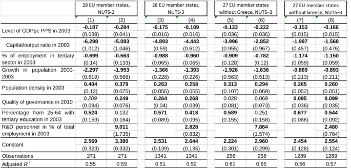
Table 1: Conditional convergence analysis
Source: Authors’ calculation. Note: The dependent variable is GDP per capita at PPS growth in 2003- 17. Huber-White-Hinkley heteroskedasticity consistent standard errors are in parentheses. Bold estimates are statistically significant at 1 percent level, an estimate in italics is statistically significant at 2 percent level.
All independent variables included exhibit the sign we would expect according to economic theory. All other things being equal, growth in GDP per capita from 2003 to 2017 was (i) lower for countries with higher initial levels of PPS GDP per capita; (ii) decreasing in the starting level of capital to output ratio; (iii) decreasing in the initial share of employees in the tertiary sector; (iv) decreasing in the rate of population growth from 2000 to 2003; (v) increasing with the starting level of population density; (vi) increasing in the quality of government indicator; (vii) increasing in the percentage of the population with higher education levels. It is reassuring that these variables, which have a theoretical rationale, are found to have a statistically significant influence on economic developments3.
As a robustness check, we included R&D personnel as a share of total employment, with statistically significant estimates. When including this variable, the percent of the population with higher education levels lost its statistical significance when using NUTS-2 data (columns
3 Other variables, which were tested but were not significant, included business demographics, health indicators and a dummy for whether a region is rural.
(1) (2) (3) (4) (5) (6) (7) (8)
-0.187 -0.284 -0.175 -0.189 -0.133 -0.222 -0.153 -0.166
(0.039) (0.041) (0.016) (0.016) (0.036) (0.036) (0.015) (0.015)
-6.298 -5.083 -4.893 -4.443 -3.996 -2.852 -1.997 -1.568
(1.012) (1.046) (0.59) (0.612) (0.955) (0.967) (0.457) (0.476)
-0.699 -0.563 -0.988 -0.960 -0.909 -0.782 -1.174 -1.150
(0.14) (0.133) (0.065) (0.065) (0.128) (0.12) (0.059) (0.059)
-2.297 -1.953 -1.366 -1.393 -1.926 -1.636 -0.869 -0.893
(0.619) (0.568) (0.228) (0.226) (0.563) (0.513) (0.213) (0.211)
0.404 0.379 0.263 0.258 0.313 0.294 0.265 0.260
(0.12) (0.075) (0.056) (0.055) (0.107) (0.069) (0.052) (0.051)
0.209 0.249 0.264 0.268 0.028 0.069 0.095 0.099
(0.084) (0.076) (0.04) (0.039) (0.081) (0.073) (0.036) (0.035)
0.524 0.132 0.571 0.418 0.589 0.251 0.677 0.544
(0.159) (0.164) (0.089) (0.095) (0.155) (0.158) (0.086) (0.092)
9.011 2.828 7.864 2.480
(1.735) (0.832) (1.574) (0.764)
2.569 3.380 2.531 2.644 2.224 2.960 2.454 2.554
(0.323) (0.332) (0.139) (0.135) (0.301) (0.299) (0.128) (0.124)
Observations 271 271 1341 1341 258 258 1289 1289
Adjusted R2 0.55 0.59 0.51 0.52 0.61 0.65 0.56 0.57
Constant
Percentage from 25-64 with tertiary education in 2003 R&D personnel in % of total employment in 2003
Capital/output ratio in 2003
% of employment in tertiary sector in 2003
Growth in population 2000- 2003
Population density in 2003 Quality of governance in 2010 Level of GDPpc PPS in 2003
28 EU member states, NUTS-2
28 EU member states, NUTS-3
27 EU member states without Greece, NUTS–2
27 EU member states without Greece, NUTS–3
(2) and (6) of Table 1), but retained its significance when using NUTS-3 data (columns (4) and (8)). This result suggests that the larger number of observations and the consequent larger variation between NUTS-3 regions than between NUTS-2 regions allow the impact of a larger set of growth drivers to be uncovered.
The residuals of our regressions correspond to the part of economic growth left unexplained by the variables we included, which we call ‘unexplained economic growth’. This
corresponds to ‘extra growth’ in addition to the growth that would have been explained by the fundamental growth determinants we considered.
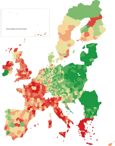
The comparison of regional ranking according to actual economic growth (Figure 1) and unexplained economic growth (Figure 2) reveals major differences. For example, actual economic growth in most Italian regions was rather poor and thus most of Italy is in red on Figure 1. But part of this poor performance was the consequence of unfavourable
fundamentals, since when we control for growth determinants, several Italian regions are in yellow (implying average performance) and some are even in green (implying good growth performance) in Figure 2.
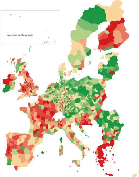
Bulgaria provides a contrary example: its actual growth performance was outstanding, as indicated by mostly green-coloured regions in Figure 1. But Figure 2, which shows
unexplained economic growth, shows that some regions had average or poor growth performance. In other words, given the initial conditions of several Bulgarian regions, economic growth should have been faster than what actually happened.
Figure 1: Actual economic growth by NUTS-3 regions, 2003-2017
Source: Authors’ calculation. Note: The figure shows the declines of GDP per capita at PPS growth in 2003-17 in the EU. The ten deciles are discriminated by alternative colours and ordered from dark red (least growing decile) to dark green (fastest growing decile).
Figure 2: Unexplained economic growth by NUTS-3 regions, 2003-2017
Source: Authors’ calculation. Note: The figure shows the declines of unexplained economic growth defined as the residual from regression (4) of Table 1. The ten deciles are discriminated by alternative colours and ordered from dark red (least growing decile) to dark green (fastest growing decile).
Among the 1341 NUTS-3 regions included in regression (4) of Table 1, the top 134 regions comes from 23 countries, highlighting that there are rather successful regions, in terms of unexplained economic growth, in most EU countries. The unlucky group of 134 worst regions is from 16 countries, suggesting more concentration. In particular, 44 of the 52
Greek regions are in the bottom decile, three are in the second worst decile and two are in the third worst decile, highlighting that Greece suffered massively after 2008.
Greece experienced a very different economic evolution during the period 2003-17 compared to other EU countries because of the divergence in terms of macroeconomic fundamentals and the austerity measures implemented after the 2008 global financial crisis.
These, in turn, had repercussions for the performance of each Greek local entity. For this reason, we re-estimated our models excluding Greece (third and fourth blocks of Table 1).
Interestingly, quality of government loses its statistical significance when the sample does not include Greece when using NUTS-2 level data, but it is highly statistically significant when using NUTS-3 level data. This result again highlights the benefits of using a larger sample. Because of the particular circumstances of the Greek economic and social collapse after 2008, we use model (6) without Greece considering NUTS-2 data and model (8) without Greece considering NUTS-3 data as our baseline scenarios for further analysis.
4 Learning from the project characteristics that could produce the best results
In this section, we compare our estimates of unexplained economic growth with the regions’ cohesion policy project characteristics, in an attempt to uncover interesting patterns. Similarly to the difficulties in detecting causal patterns in literature, we cannot claim causality either, ie that certain cohesion project characteristics explain this extra growth. Other factors might be more important for growth development. For example, on the positive side, that the government attracted large foreign direct investment which boosted production and average productivity in the region; or on the negative side, that there was a major natural disaster. Nevertheless, it is instructive to analyse the best and worst performing regions in terms of the different characteristics of cohesion policy projects. We also discuss certain factors that could explain the associations we found.
4.1 Methodology
We conducted two types of analysis:
1. A correlation analysis across the whole EU, in which we considered all the regions simultaneously to see how their characteristics are correlated with unexplained economic growth, and
2. A quartile analysis by country, in which we contrasted only the best and worst performers within each country, and then averaged the differences across the EU.
Both approaches have a rationale. Correlation analysis of the full sample of regions can highlight patterns systematically over all regions of the EU. However, it is possible that the association between project characteristics and unexplained economic growth is stronger for the best and the worst performers, but less so for those regions which are in the middle of the growth distribution. Furthermore, country-specific characteristics can also play a role.
Therefore, in our second analysis we calculated the difference in project characteristics of the best and worst performing regions for each country, and then averaged these country- specific differences across the EU. Since countries differ in terms of the number of NUTS-2 regions, we considered only those EU countries that have at least four NUTS-2 regions. We considered the top quartile of regions to be the best performers and the bottom quartile of regions to be the worst performers in terms of unexplained economic growth4. As a
robustness check, we analysed NUTS-3 regions where data is available.
4.2 Project characteristic data
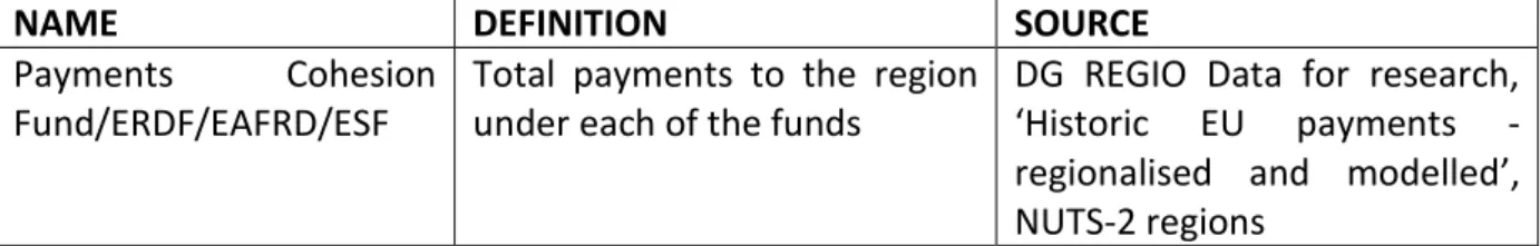
The publicly available data on project characteristics can be grouped essentially into three categories: payments by EU fund, interregional project characteristics and summary project characteristics (including sectoral breakdown).
Payments by fund to each region are available via the DG REGIO Data for research platform (https://ec.europa.eu/regional_policy/en/policy/evaluations/data-for-research/) under the name ‘Historic EU payments – regionalised and modelled’5. The 2014-2020 cohesion funds are split between the European Regional Development Fund (ERDF, 55 percent of total cohesion spending), the European Social Fund (ESF, 23 percent), the Cohesion Fund (CF, 20 percent) and the Youth Employment initiative (1 percent). The European Agricultural Fund
4 That is, when a country has four NUTS-2 regions, then only the best and the worst regions are considered, but when, for example, a country has 12 NUTS-2 regions, we consider the top three and the bottom three regions.
for Rural Development (EAFRD) is part of the Common Agricultural Policy (CAP), but since the EAFRD has a regional focus, we also considered this fund in our analysis. EAFRD is also part of the European Structural and Investment Funds (ESIF), along with the ERDF, ESF, CF and the European Maritime and Fisheries Fund (EMFF)6.
On project characteristics, however, readily available public data at regional level is scarce.
The European Commission aggregates data at programme level, not allowing for detailed regional comparisons. We therefore used two datasets, which we refer to as the 4P dataset and the interregional database. Neither is complete in its coverage of projects, but both provide different insights into project characteristics conducive to analysis of unexplained economic growth.
One data source, which we designate the ‘4P dataset’, comes from the European Commission Regional Policy website (https://ec.europa.eu/regional_policy/en/atlas/), where up to four projects per NUTS-2 region are listed and explained in detail. These same projects can be found by accessing https://cohesiondata.ec.europa.eu/projects, where it states “This is a list of representative projects funded by ESIF. It is not an exhaustive list of all projects”. We have to presume that the sample is indeed representative of projects, even though it is not representative of the funds: of the 606 projects listed, 504 are funded by the ERDF, 51 by the CF, 11 by the ESF, and two by the pre-accession instrument, while the fund is not indicated for 38 projects7. However, as long as the criteria for selecting projects is not related to the characteristics analysed, or to unobservables that affect unexplained
economic growth, the correlations should still convey significant information8. The 606 projects refer to the 2007-2013 Multiannual Financial Framework (MFF) period and their combined budget amounts to 3.2 percent of the total ESIF budget in 2007-2013, a relatively low share.
The other dataset, which we designate as the ‘interregional dataset’
(https://www.keep.eu/), contains projects from interregional programmes from the ERDF.
6 Information about ESIF: https://ec.europa.eu/info/funding-tenders/funding-opportunities/funding- programmes/overview-funding-programmes/european-structural-and-investment-funds_en.
7 While there are 606 unique projects in this dataset, many of them are interregional and thereby altogether there are 896 project+region pairs. In our analysis we consider an interregional project for each region it targets.
8 This argument is analogous to the justification of the use of instrumental variables in econometrics.
These include cross-regional initiatives (within a country) and international initiatives. We focus on data from the 2007-2013 period, for which the database includes 10,089 projects in total, corresponding to 94 percent of the total number of interregional projects under the ERDF in this programming period – thus its coverage is almost complete.
It should be noted that these two datasets relate to different sets of projects. The
interregional dataset covers only projects that involved interregional cooperation and that were ERDF-funded, while the 4P dataset covers projects from all ESIF funds (even though it is dominated by the ERDF, as we noted above), and these projects can be of any type, either region specific or interregional. Thus, findings might not necessarily point in the same direction. See the annex for the definition of the variables we were able to construct from these sources.
4.3 Correlation analysis Fund type
It is first important to highlight that cohesion policy commitments remain tied to the level of regional development. For example in the 2014-2020 programming period, on average, less- developed regions (with GDP per capita at PPS below 75 percent of the EU average)
received 1.61 percent of regional nominal GDP, transition regions (GDP per capita at PPS between 75 percent and 90 percent of the EU average) received 0.31 percent of GDP, while more developed regions (with GDP per capita at PPS over 90 percent of the EU average) received only just 0.07 percent as a share of GDP from ERDF and ESF combined.
Furthermore, only countries with GDP per capita below 90 percent of the EU average are eligible for Cohesion Fund payments, which further increases the amounts received by less- developed and transition regions, by on average 0.53 percent of GDP.
Given the low amounts as a share of GDP, it is unlikely that EU cohesion funds have a material impact on GDP growth in more developed regions. Therefore, as a robustness analysis, we studied the association between unexplained economic growth and project characteristics by excluding more developed regions. We found that our results are robust.
Table 2 shows that the funding received by a region under the Cohesion Fund is highly statistically significant when considering the correlation with a region’s unexplained economic growth, with the correlation being positive. The absolute value of the amount paid into a region had a correlation of 0.272 with unexplained economic growth when all regions are considered, and 0.349 when developed regions are excluded. In contrast, the point estimate of the correlation coefficient is negative for the other three funds, though only marginally significant in the case of the ESF. A possible explanation for these results for the other three funds could be their more diverse goals, including environmental protection and social inclusion, which might not immediately lead to faster economic growth.
Table 2: Correlation between unexplained economic growth and funds received, NUTS-2
All regions Developed regions excluded
ERDF -0.058 -0.135
(0.359) (0.202)
ESF -0.117 -0.179
(0.063) (0.090)
CF 0.272 0.349
(0.011) (0.004)
EAFRD -0.026 -0.129
(0.676) (0.230)
Source: Authors’ calculation. Note: Correlation coefficient refers to the estimated correlation
between unexplained economic growth and funds received in euros at the NUTS-2 level (NUTS-3 level data is not available). The p-value is reported in brackets, which shows the probability of finding the observed (or larger in absolute terms) correlation coefficient when it is actually zero. Thereby, a low p-value indicates evidence for a non-zero correlation coefficient. Bold numbers indicate estimates which have a p-value below 0.1, that is, which are statistically significant at the 10 percent level.
Interregional projects
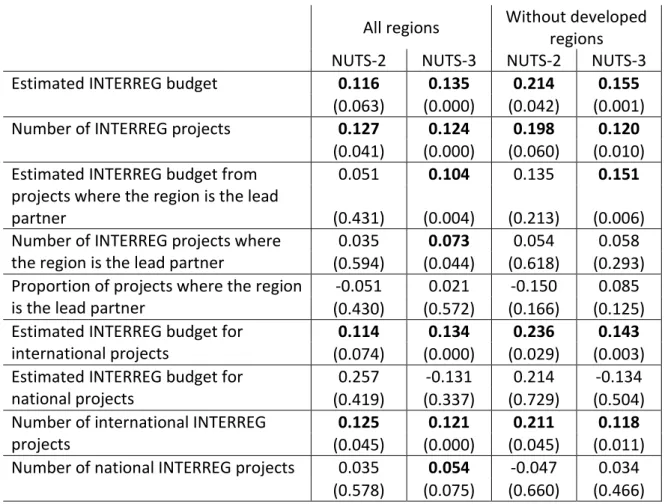
Although the funds received under the ERDF as a whole are not statistically associated with unexplained economic growth, projects under the interregional umbrella do appear to be correlated. Table 3 shows how the total number of interregional projects and estimates of how much budget goes into the region correlate positively with the region’s unexplained economic growth. The estimated correlation coefficients are statistically larger than in all samples: with and without developed regions, and at both NUTS-2 and NUTS-3 levels. Table
3 also shows that participation in interregional projects matters more than their leadership:
the three indicators related to leadership of interregional projects are generally not statistically significantly correlated with unexplained economic growth, only three of the twelve correlation coefficient estimates are statistically significant. Interregional projects might foster the cooperation and knowledge exchange between various regions, which might explain their positive contribution.
By distinguishing between international (connecting regions from different countries) and national (connecting two or more regions from the same country) interregional projects, we find that only international interregional projects are positively, and in a statistically
significant way, associated with better economic performance. Both the budget and the number of such projects are positively related to growth in all four alternative samples included in Table 3. In contrast, the budget of purely national projects is never significantly associated with better economic performance, and in some specifications the direction of association is even negative, while the number of national projects is significant in only one of the four cases.
Table 3: Correlation between unexplained economic growth and various indicators related to interregional funds
All regions Without developed regions
NUTS-2 NUTS-3 NUTS-2 NUTS-3
Estimated INTERREG budget 0.116 0.135 0.214 0.155
(0.063) (0.000) (0.042) (0.001) Number of INTERREG projects 0.127 0.124 0.198 0.120
(0.041) (0.000) (0.060) (0.010) Estimated INTERREG budget from
projects where the region is the lead partner
0.051 0.104 0.135 0.151 (0.431) (0.004) (0.213) (0.006) Number of INTERREG projects where
the region is the lead partner
0.035 0.073 0.054 0.058 (0.594) (0.044) (0.618) (0.293) Proportion of projects where the region
is the lead partner
-0.051 0.021 -0.150 0.085 (0.430) (0.572) (0.166) (0.125) Estimated INTERREG budget for
international projects
0.114 0.134 0.236 0.143 (0.074) (0.000) (0.029) (0.003) Estimated INTERREG budget for
national projects
0.257 -0.131 0.214 -0.134 (0.419) (0.337) (0.729) (0.504) Number of international INTERREG
projects
0.125 0.121 0.211 0.118 (0.045) (0.000) (0.045) (0.011) Number of national INTERREG projects 0.035 0.054 -0.047 0.034
(0.578) (0.075) (0.660) (0.466) Source: Authors’ calculation. Note: Correlation coefficient refers to the estimated correlation between unexplained economic growth and various indicators related to interregional funds (as indicated in the row labels). The p-value is reported in brackets; see its explanation in the note to Table 2.
Most likely, resorting to long-distance partnerships might bring about efficiency gains for project design, procedures and implementation. In order to engage in cross-border cooperation, partners probably consider more ambitious and far-reaching projects, since otherwise the extra administrative burden to work together with entities from other countries might not be worthwhile. Cross-border cooperation potentially provides fruitful knowledge transfers, which could be valuable both between regions at similar levels of development and between regions with different levels of development, thereby helping less-developed regions to learn from their luckier peers. Importantly, projects involving partners from two or more different countries could be less likely to be prone to corruption and waste of resources, as institutions and businesses find themselves outside their usual
network of relationships and in new, unfamiliar environments, where playing by the rules could be the safest and most rational choice.
Summary project characteristics
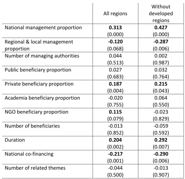
One of the strongest positive associations is between unexplained economic growth and the proportion of projects managed at national level (as opposed to regional and local levels;
Table 4). This might be because of relatively weak local institutions in countries with more room for convergence (eg eastern countries), where central ministries possibly are better at absorbing and managing EU funds. At the same time, national entities might be more able to identify and prioritise projects with the greatest potential.
Regions with a higher proportion of projects whose primary beneficiary is a private company also perform better. This might be because projects targeting companies are more return- driven and can unlock economic growth, but it might simply be a sign of regions with more positive growth prospects – where more companies exist and thus apply for funds. In our models of unexplained economic growth, we tried to control for business demographics (such as birth and death rates of businesses, the population of active enterprises, and employees in the population of active enterprises), and found it not to be a significant factor.
Regions with higher proportions of projects whose primary beneficiary is a non-research NGO also perform better, but only when the full sample is used. When we restrict the sample to less-developed and transition regions, the correlation coefficient is no longer significant. The positive association with non-research NGOs could suggest that such
beneficiaries might be able to mobilise local participants. It is important to highlight that the share of public-sector beneficiaries is not associated with better growth outcomes.
Duration in the 4P dataset is strongly positively associated with unexplained economic growth, potentially hinting at the positive effects of taking a longer-term view of
investments. The result for longer-duration projects suggests that more strategic projects could bring benefits.
We find a strong negative association between the national co-financing rate and unexplained economic growth, with a -0.217 correlation coefficient for all regions and - 0.290 for the subsample without regions. That is, regions with higher national co-financing rates tend to grow less. This finding might be explained by the availability of funding: when the national co-financing rate is low, national authorities might have more resources to spend on other projects, which might stimulate growth.
Table 4: Correlation between unexplained economic growth and summary project characteristics (4P dataset), NUTS-2 regions
All regions
Without developed
regions
National management proportion 0.313 0.427
(0.000) (0.000)
Regional & local management proportion
-0.120 -0.287
(0.068) (0.006)
Number of managing authorities 0.044 0.002
(0.513) (0.987)
Public beneficiary proportion 0.027 0.032
(0.683) (0.764)
Private beneficiary proportion 0.187 0.215
(0.004) (0.043)
Academia beneficiary proportion -0.020 0.064
(0.755) (0.550)
NGO beneficiary proportion 0.115 -0.023
(0.079) (0.829)
Number of beneficiaries -0.013 -0.059
(0.852) (0.592)
Duration 0.204 0.292
(0.002) (0.007)
National co-financing -0.217 -0.290
(0.001) (0.006)
Number of related themes -0.044 -0.013
(0.500) (0.907)
Source: Authors’ calculation. Note: Correlation coefficient refers to the estimated correlation
between unexplained economic growth and various indicators related to project characteristics from the 4P dataset (as indicated in the row labels). The p-value is reported in brackets; see its explanation in the note to Table 2.
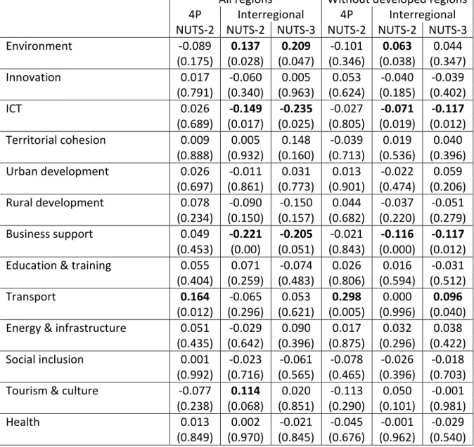
Sectoral breakdown of projects
In terms of the association of sectors with unexplained economic growth, no clear patterns emerge and the results are conflicting when using the two alternative datasets for project characteristics (Table 5). The estimated correlation coefficients are rarely significant, and when this is the case for a particular sample, the coefficient is not significant for other samples. Perhaps the strongest association is with the transport sector for which three of the six samples resulted in statistically significant positive correlation coefficients, yet the other three samples resulted in insignificant estimates. Somewhat surprisingly, business support is negatively associated with unexplained economic growth in the interregional dataset, but such estimates are insignificant for the 4P dataset. Three of the six estimates for environment are significantly positive, but not the other three, of which two even have negative point estimates. For the other sectors, estimates are not significant and often the sign of the point estimate differs for the two datasets. These findings suggest that the sector of intervention is probably less relevant for economic growth.
Table 5: Correlation between unexplained economic growth and sector breakdown of projects
All regions Without developed regions 4P Interregional 4P Interregional
NUTS-2 NUTS-2 NUTS-3 NUTS-2 NUTS-2 NUTS-3
Environment -0.089 0.137 0.209 -0.101 0.063 0.044
(0.175) (0.028) (0.047) (0.346) (0.038) (0.347)
Innovation 0.017 -0.060 0.005 0.053 -0.040 -0.039
(0.791) (0.340) (0.963) (0.624) (0.185) (0.402)
ICT 0.026 -0.149 -0.235 -0.027 -0.071 -0.117
(0.689) (0.017) (0.025) (0.805) (0.019) (0.012)
Territorial cohesion 0.009 0.005 0.148 -0.039 0.019 0.040
(0.888) (0.932) (0.160) (0.713) (0.536) (0.396)
Urban development 0.026 -0.011 0.031 0.013 -0.022 0.059
(0.697) (0.861) (0.773) (0.901) (0.474) (0.206)
Rural development 0.078 -0.090 -0.150 0.044 -0.037 -0.051
(0.234) (0.150) (0.157) (0.682) (0.220) (0.279)
Business support 0.049 -0.221 -0.205 -0.021 -0.116 -0.117
(0.453) (0.00) (0.051) (0.843) (0.000) (0.012)
Education & training 0.055 0.071 -0.074 0.026 0.016 -0.031
(0.404) (0.259) (0.483) (0.806) (0.594) (0.512)
Transport 0.164 -0.065 0.053 0.298 0.000 0.096
(0.012) (0.296) (0.621) (0.005) (0.996) (0.040)
Energy & infrastructure 0.051 -0.029 0.090 0.017 0.032 0.038
(0.435) (0.642) (0.396) (0.875) (0.296) (0.422)
Social inclusion 0.001 -0.023 -0.061 -0.078 -0.026 -0.018
(0.992) (0.716) (0.565) (0.465) (0.396) (0.703)
Tourism & culture -0.077 0.114 0.020 -0.113 0.050 -0.001
(0.238) (0.068) (0.851) (0.290) (0.101) (0.981)
Health 0.013 0.002 -0.021 -0.045 -0.001 -0.029
(0.849) (0.970) (0.845) (0.676) (0.962) (0.540)
Source: Authors’ calculation. Note: Correlation coefficient refers to the estimated correlation
between unexplained economic growth and percentage of projects, which include the sector listed on the row labels among its related themes. The p-value is reported in brackets; see its explanation in the note to Table 2.
4.4 Quartile analysis
It is useful to complement our analysis by focusing on the differences between the best and worst performers, in terms of unexplained economic growth, from each country. The association between project characteristics and unexplained economic growth could be stronger for the best and the worst performers, but less so for those regions in the middle
of the growth distribution. Country-specific characteristics could also play a role. Therefore, in this section, we calculate the differences in terms of the project characteristics of the best and worst performing regions for each country, and then average these country-specific differences across the EU. Thus, any eventual idiosyncratic country-specific factor is eliminated.
We consider only those EU countries that have at least four NUTS-2 regions and regard the best performers as those in the top quartile of regions and the worst performers as those in the bottom quartile of regions, in terms of unexplained economic growth. In principle, these results could be at odds with the correlations that include all regions, as reported in section 4.3, because they only refer to less than half of the total sample and, by design, do not consider the dynamics within the middle of the distribution. However, in practice our results are very much in line with the simple correlation analysis (Table 6), suggesting the
robustness of our results.
The most robust characteristics suggest that the best performing regions have, on average, projects with:
(i) Longer durations,
(ii) More inter-regional focus,
(iii) A higher proportion of private sector or non-research NGOs or academic entities among the beneficiary entities (as opposed to public-sector entities),
(iv) A higher share of funding from the Cohesion Fund, (v) A higher share of EU co-financing.
We do not include the share of national vs. regional/local management of projects in this analysis, because in several countries (Belgium, Czech Republic, France, Germany, Hungary, Netherlands and Portugal) there is very little within-country variability in this indicator. The exclusion of these countries from the analysis, along with the exclusion of those countries that have fewer than four NUTS-2 regions, eliminates most of the observations. Hence, for
the analysis of national vs. regional/local management of projects, we only rely on the correlation analysis presented in section 4.3.
Similarly to the correlation analysis of Section 4.3, no clear patterns emerge for the sectors of intervention and the results are conflicting when using the two alternative datasets for project characteristics9.
Table 6: Differences in project characteristics between the first and the last quartiles of regions by country concerning unexplained economic growth
Source: Authors’ calculation. Note: we first calculate differences of the project characteristics of the best and worst performing regions for each country, and then average these country-specific differences across the EU.
5. Summary and policy implications
The academic literature on the effectiveness of European Union cohesion policy is inconclusive and there are major problems with earlier methodologies, and in particular, with the analysis of causality. Additionally, while many papers focused on the overall impact of cohesion policy, very few works have looked at the characteristics of cohesion projects.
9 Detailed results are available from the authors on request.
Funding from: ERDF interregional projects:
ERDF -0.18 Estimated INTERREG budget NUTS-2 0.13
ESF -0.10 Estimated INTERREG budget NUTS-3 0.65
CF 0.11 Number of INTERREG projects NUTS-2 0.14
EAFRD -0.42 Number of INTERREG projects NUTS-3 0.55
Estimated INTERREG budget from projects where the region is the lead partner NUTS-2
0.01
4P dataset: Estimated INTERREG budget from projects where
the region is the lead partner NUTS-3
0.42 Private beneficiary proportion 0.10 Number of INTERREG projects where the region is
the lead partner NUTS-2
-0.08 NGO beneficiary proportion 0.48 Number of INTERREG projects where the region is
the lead partner NUTS-3
0.22 Public beneficiary proportion -0.11 Proportion of projects where the region is the lead
partner NUTS-2
0.32 Academia beneficiary proportion 0.51 Proportion of projects where the region is the lead
partner NUTS-3
0.19
Duration 0.07 Duration NUTS-2 0.05
National co-financing -0.10 Duration NUTS-3 0.09
We have therefore adopted a novel methodology that first estimated ‘unexplained economic growth’ by controlling for the influence of various region-specific factors, and then analysed its relationship with about two dozen characteristics specific to projects carried out in various regions in the context of EU cohesion policy. We found that the best- performing regions have on average projects with longer durations, more inter-regional focus, lower national co-financing, more national (as opposed to regional and local) management, higher proportions of private or non-profit participants among the
beneficiaries (as opposed to public-sector beneficiaries) and higher levels of funding from the Cohesion Fund. No clear patterns emerged concerning the sector of intervention.
Our results have several implications for EU cohesion policy reform, of which we highlight four.
First, the beneficial effects of longer duration are consistent with the importance of strategic focus in cohesion policy. Setting up long-term strategies and sticking to them in implementation seem to be important factors in the usefulness and effectiveness of cohesion that do not require high levels of flexibility. In contrast the adopted European Union budget for 2021-2027 includes various forms of flexibility, including moving resources between priorities, years or even between spending categories10.
Second, one of the most robust findings from our study is the great potential of interregional projects to unlock growth. Yet only a limited share of EU cohesion policy projects connect regions: the total budget of such projects was just 4.8 percent of the ERDF spending in the 2007-2013 MFF, and hence we recommend allocating more for such
projects. However, care must be taken to avoid divergent tendencies that can arise if more- advanced regions are better able to engage in large-scale cooperation. Capacity building becomes crucial, in which fostering cooperation between more and less-developed regions plays a useful role.
10 See the adopted 2021-2027 European Union budget at: https://ec.europa.eu/info/publications/adopted- mff-legal-acts_en. In general, flexibility within the EU budget can be useful to respond to unforeseen circumstances, such as the 2015 migration crisis. But our findings refute the need for high levels of flexibility
Third, our empirical finding which shows that higher national co-financing is associated with lower economic growth likely reflects the role of fiscal constraints after the 2008 global financial crisis, since higher national contributions leave less scarce public resources for other spending priorities. Yet in countries that do not face fiscal constraints, higher national co-financing might even lead to an increase in cohesion projects, because for a given
amount of EU funding more national funding is added. Thus, the extent of fiscal constraints, or the lack of it, could be a factor in determining the co-financing rate11.
And fourth, the importance of a locally-led perspective should be reconciled with our finding of better centralised management. A possible way to do this would be to couple locally-led demand for projects, driven by more accurate knowledge of local needs and deficiencies, with higher-level allocation, oversight and management. Perhaps our empirical finding of weaker local management results from inadequate administrative capacity at local level – our econometric estimates also confirmed a statistically significant and robust relationship between economic growth and an indicator of institutional quality, which could reflect administrative capacity too. Hence, where administrative capacity is lacking, building proper expertise and structures should be a top priority.
References
Bachtler, J., I. Begg, D. Charles and L. Polverari (2013) Evaluation of the Main Achievements of Cohesion Policy Programmes and Projects over the Long Term in 15 Selected Regions, 1989–2012, Final Report to the European Commission, European Policies Research Centre, University of Strathclyde and London School of Economics,
11 Another aspect of setting the co-financing rate relates to the additionality principle. While the December 2013 Regulation (EU) No 1303/2013 of the European Parliament and of the Council re-confirmed this principle for cohesion policy (“In order to ensure a genuine economic impact, support from the Funds should not replace public or equivalent structural expenditure by Member States”), Varblane (2016) concluded that EU funds replaced the Baltic countries’ own funding of higher education research. If a comprehensive analysis of the observation of this principle in the case of all countries and sectors finds violations, then a higher national co- financing rate would be justified, in order to direct some of the national resources back to the funding of regional and cohesion projects.
http://ec.europa.eu/regional_policy/sources/docgener/evaluation/pdf/eval2007/cohesion_
achievements/final_report.pdf
Bachtler, J., I. Begg, D. Charles and L. Polverari (2017) ‘The long-term effectiveness of EU cohesion policy. Assessing the achievements of the ERDF, 1989–2012’, in J. Bachtler, P.
Berkowitz, S. Hardy and T. Muravska (eds) EU cohesion policy. Reassessing performance and direction, Routledge, London,
https://www.taylorfrancis.com/books/10.4324/9781315401867
Berkowitz, P., Monfort, P., and Pieńkowski, J. (2020) ‘Unpacking the growth impacts of European Union Cohesion Policy: Transmission channels from Cohesion Policy into economic growth’, Regional Studies, 54(1), 60-71,
https://doi.org/10.1080/00343404.2019.1570491
Charron, N., L. Dijkstra and V. Lapuente (2014) ‘Regional governance matters: Quality of government within European Union member states’, Regional Studies, 48(1), 68-90, https://doi.org/10.1080/00343404.2013.770141
Crescenzi, R. and M. Giua (2017) ‘Different approaches to the analysis of EU cohesion policy’, in J. Bachtler, P. Berkowitz, S. Hardy and T. Muravska (eds) EU cohesion policy.
Reassessing performance and direction, Routledge, London, https://www.taylorfrancis.com/books/10.4324/9781315401867
Hagen, T. and P. Mohl (2009) ‘Econometric evaluation of EU cohesion policy – A survey’, Discussion Paper No. 09-052, Zentrum für Europäische Wirtschaftsforschung (ZEW), http://ftp.zew.de/pub/zew-docs/dp/dp09052.pdf
Marzinotto, B. (2012) ‘The growth effects of EU cohesion policy: A meta-analysis’, Working Paper 2012/14, Bruegel, http://bruegel.org/2012/10/the-growth-effects-of-eu-cohesion- policy-a-meta-analysis/
Percoco, M. (2017) ‘Impact of European Cohesion Policy on regional growth: does local economic structure matter?’, Regional Studies 51(6), 833-843,
https://doi.org/10.1080/00343404.2016.1213382
Pieńkowski, J. and P. Berkowitz (2015) ‘Econometric assessments of cohesion policy growth effects: How to make them more relevant for policy makers?’ Regional Working Paper 02/2015, European Commission, Directorate-General for Regional and Urban Policy, https://ec.europa.eu/regional_policy/en/information/publications/working-
papers/2015/econometric-assessments-of-cohesion-policy-growth-effects-how-to-make- them-more-relevant-for-policy-makers
Rodríguez-Pose, A. and E. Garcilazo (2015) ‘Quality of Government and the Returns of Investment: Examining the Impact of Cohesion Expenditure in European Regions’, Regional Studies 49(8), 1274-1290, https://doi.org/10.1080/00343404.2015.1007933
Solow, R.M. (1956) ‘A contribution to the theory of economic growth’, Quarterly Journal of Economics 70(1), 65-94, https://doi.org/10.2307/1884513
Swan, T.W. (1956) ‘Economic growth and capital accumulation’, Economic Record 32(2), 334–361, https://doi.org/10.1111/j.1475-4932.1956.tb00434.x
Varblane, U. (2016) ‘EU structural funds in the Baltic countries: useful or harmful?’ Estonian Discussions on Economic Policy 24(2), 120-137,
https://ojs.utlib.ee/index.php/TPEP/article/view/13098/8175