Reinvestment of earnings in Polish FDI in fl ows

Reinvestment of earnings in Polish FDI in fl ows

ANETA KOSZTOWNIAK

Department of Economic Policy and Banking, Economics and Finance Faculty, Kazimierz Pulaski University of Technology and Humanities in Radom, ul. Chrobrego 31, 26-600 Radom, Poland

Received: June 4, 2019 • Revised manuscript received: September 12, 2020 • Accepted: December 15, 2020

© 2021 Akademiai Kiado, Budapest

ABSTRACT

The aim of this paper is to diagnose the cause-and-effect relationships between reinvestment of earnings (RoE) and other components of FDI inflows and GDP in Poland in the years of 2004–2019, using the VECM model^pp. Changes in the structure of FDI inflows in Poland are in line with the stages of the FDI life cycle. The increase in the share of RoE in the structure of these investments is also accompanied by an increase in the impact and the degree of explanation of changes in GDP. Studies confirmed that changes in the structure of FDI in Poland was adequate to the theoretical cycle of FDI life. The increase in the share of RoE in the structure of FDI inflows is accompanied by a decrease in equities. The VECM model, impulse response function and decomposition analysis confirmed that among FDI components mainly equities, and next, RoE have large participation in the degree of explanation of GDP. In the short-term, mainly equity has the most important impact on GDP, and additionally, RoE. In the long-time, the importance of equity decreases, while increases the impact of RoE, and also, debt instruments. The increase in the share of RoE in the structure of FDI inflows accompanied by the increase in the impact of these investments on GDP changes.

KEYWORDS

FDI, reinvestment of earnings, GDP, Poland, VECM, the response function, variance decomposition JEL CLASSIFICATION INDICES

C50, C52, F41, F43, O11

pCorresponding author. E-mail: a.kosztowniak@uthrad.pl

ppThe views expressed in this study are the views of the author and do not necessarily reflect those of National Bank of Poland.

1. INTRODUCTION

FDI inflows consist of three components: equity capital, reinvestment of earnings (reinvested earnings, RoE) and intercompany debt flows as debt instruments. These financial components of FDI depend on the investment strategy of foreign investors which are made with the knowledge of internal determinants of their companies’development and location conditions in the host country. The structure of the FDI inflows changes according to the phases of the FDI life cycle.

Nearly 60 years of capital expansion in the form of FDI in the Polish economy shows changes in the structure of these investment. In the global FDI inflows, the share of RoE and debt instruments is growing compared to the decline in the share of equity capital. The RoE of non-financial enterprises, e.g., greenfields are particularly important impetus for economic growth. The increase in these reinvestments assures the expansion of property investments, e.g., production factories. This is also a signal of intentions to continue the investment in the future in a favourable climate of the host country.

The aim of this paper is to analyse the cause-and-effect relationships between RoE and other components of FDI inflows and GDP in Poland in the years 2004–2019, using the VAR/VECM model.

We examine:

1. Are the changes in the structure of FDI in Poland during 2004–2019 adequate to the theoretical cycle of the FDI life?

2. Whether the increase in the share of RoE in the structure of FDI inflows was accompanied by a decrease in equities and other forms of capital participation?

3. Whether the increase in the share of RoE in the structure of FDI inflows was accompanied by the increase in the impact of these investments on changes in GDP?

Our hypothesis is that changes in the structure of FDI inflows in Poland are in line with the phases of the FDI life cycle. The increase in the share of RoE in the structure of these in- vestments is also accompanied by an increase in the impact and the degree of explanation of changes in GDP.

This study is organised as follows. After the introduction, Section 2 provides a literature review of the cycle of FDI life, main determinants of RoE and the cause-and-effect relationships between FDI and economic growth. Section 3 presents the methodology offinancial instruments of FDI, and Section 4 gives information about empirical data. Section 5 shows research pro- cedure of the econometric model and Section 6 presents the results of our analysis of VAR/

VECM, impulse response functions and also the variance decomposition. Concluding remarks are provided in Section 7.

2. RELATED LITERATURE

The amount of RoE in the host countries is significantly influenced by: 1) the life cycle of FDI, 2) economic growth conditions and 3) tax regulations.

Theoretical literature focuses on the impact of FDI (all components) on economic growth and mutual relations in the global perspective. These were not theoretical and empirical studies

on the impact of financial structure of FDI (individual components) on the economic growth of the investor’s countries of origin and host countries.

The distinction between the components of FDI in the literature is found mainly in the so- called FDI profitability cycle. This cycle refers to the accumulated FDI inflows, i.e., to FDI in- ward stock, and thus, to the component of reinvested profits. According to Brada –Tomsik (2003), the profitability life cycle of FDI has three-stages. This profitability path of FDI refers to FDI inward stock, because this is the cumulative FDI inflows value and the FDI cumulative profitability:

Stage 1 (opening) is connected with the expenditures of foreign investors in the host country and means negative profitability (increased equity),

In Stage 2 (growth), there is a profit, peaking at around the 6^thyear of the cycle (increased RoE and debt instruments),

Stage 3 (repatriation) is connected with the division of the achieved profit; the dividend is paid out and increase debt instruments, or disinvestments.

An important question is how investors decide whether to engage in FDI inflows between:

equity, RoE and debt instruments. According to Novotny – Podpiera (2008), among the countries of Central and Eastern Europe (CEE), the full-fledged FDI life cycle usually includes a period of 15 years, followed by the projection toward zero annual profitability.

Moreover, it should be noted that there is an abundant literature regarding what motivates foreign investorswhere to invest andhow much to invest, most of these studies have disregarded how these investments are financed. The World Investment Report (2008) pointed out that in the developing countries RoE accounted for about 30% of total FDI inflows as a result of increased profits of foreign affiliates. Therefore, it is very important to find out the determinants of RoE as the significant portion of FDI financial components.

One of the most outstanding analyses of reinvested earnings was conducted by Lundan (2006). She distinguished three explanatory factors: 1) Those encouraging reinvestments, i.e., a strong growth rate in a host country market and rising income levels in a given industry may signal new investment opportunities in the host market. 2) Those encouraging repatriation, i.e., higher corporate tax rates in the host country are also expected to have a deterring effect on RoE and, consequently, to accelerate the repatriation of earnings. 3) Agency consideration: Factors affecting a multinational corporation’s (MNC’s) decisions regarding the amounts of dividend payments may also encourage repatriation. For example, countries that have high market or political risks or that are culturally or institutionally different from the home country of the MNC are likely to cause high levels of repatriation.

The above-mentioned localisation conditions for RoE were analysed empirically by several researchers.Oseghale–Nwachukwu (2010) empirically proved that good governance, market size, market growth rate, exchange rate, quality of labour, and the profitability of existing op- erations are all positively correlated with RoE.Taylor et al. (2013)argued if the economic growth of a host country and the profitability of foreign firms increase, foreign investors tend to hold reinvested earnings in the country. In contrast, a depreciation of the host currency and an increase in the host country’s government consumption seem to decrease the volume of re- investments. Saloria – Brewer (2013) pointed out that RoE are likely to be associated with corporate taxes rates, exchange rates, interest rates, and the operational needs of MNC in

particular countries. They also noted that retained earnings are likely to be responsive to the restrictions on the remittance of profits to the parent company (Table 1).

In reference to the profitability cycle of FDI as well as location factors for reinvested earnings –it should be stated that their amount and changes in time depend on both the stage of in- vestment implementation (phase) and investment climate factors.

However, referring to the empirical analysis that treats FDI as a monolithic form of foreign capital, we can define the analysis as: 1) influence of FDI on GDP–with results: positively, the lack of influence or a very weak one and negatively, and 2) inter-relationships between FDI and GDP–with results: mutually-bidirectional and uni-directional.

As regards the impact of FDI on GDP, the new theories of growth assume the positive impact of capital on production growth in both short- and long-term. For examples, in the models developed by the followers of the real business cycle arguments are raised about higher productivity of FDI in comparison to domestic capital. It is emphasised that the capital spillover effects are stronger than capital diminishing returns (Liu et al. 2000; Gorynia et al. 2005; Faj- gelbaum et al. 2015;Lin–Kwan 2016;Gebrihiwet 2017).

Some empirical studies describe the positive effect of FDI on GDP of the host country (Blomstr€om 1986; De Gregorio 1992;Balasubramanyam et al. 1996;Alfaro et al. 2001;Kornecki –Raghavan 2011). FDI-friendly policies are based on the belief that FDI, apart from bringing in capital and creating jobs, has several positive effects which include productivity gains, tech- nology transfers and the introduction of new managerial skills and know-how into the domestic market (Molendowski–Polan 2013). However, other studies refer tolack of influenceor a very weak one on economic growth (Carkovic–Levine 2002,2005;Kang–Du 2005;Bacic et al. 2005;

Gorynia et al. 2015), while other studies present anegative influenceof FDI on GDP (Saltz 1992;

Mencinger 2003). It is quite important how big the correlation between FDI inflows and GDP in the host country is. If this correlation is low, then the effect of the investment on GDP is also

Table 1.Main location conditions of FDI inflows refer reinvestment of earnings/reinvested earnings in the host country

Location conditions Expected sign of the causality

Consumer confidence Positive

Legislative strengths

Country risk:financial, economic and political risk Negative Payments delays

Corporate tax (represent an extra cost)

Investment profile of host country Positive/Negative

Contract viability for direct investment enterprises GDP (value) and rate of growth

Real effective exchange rate (appreciation/depreciation)

Source: Own compilations based onPolat (2017)andSalora–Brewer (2013).

poor (Herzer et al. 2008). These findings show that FDI may harm the host economy, for instance when foreign investors claim scarce resources or reduce investment opportunities for the local investors. There is also some concern that no positive knowledge spillovers mayfinally occur within the developing countries, because multinationals will be able to protect theirfirm- specific knowledge, or because they may buy their inputs from foreign rather than local sup- pliers.

Next group of researchers studying relationships between FDI and GDP emphasised dif- ferences in their mutual inter-relationships. In some countries it is FDI which has a positive impact on GDP (Bende –Nabende et al. 2000;Nunnenkamp et al. 2007; Jarosinski –Barło- _

zewski 2019). In some others it is GDP that clearly attracts FDI inflows (Chowdhury–Mavrotas 2005).

While some authors found no significant relation between FDI and growth, others showed either an unconditional positive link between these two variables or a relationship that is conditional to particular characteristics of the host country, such as the level of human capital or the depth of the financial system. At least two reasons explain these mixed results:

First, most of the authors analysed the correlation between FDI and growth using a regression analysis framework that is silent on the causality between these two variables.

Second, in the studies that do address the causality issue, the influence of other social and economic variables is seldom taken into account directly within the model and, in many cases, these are simply ignored.

In the opinion ofCarkovic–Levine (2002), the positive effect of FDI and portfolio inflow is a result of technology transfer. They proved that FDI inflow does not affect economic growth independently.Herzer et al. (2008)argued that if FDI considerably “crowd out”domestic in- vestments, then a growth decelerating impact on the recipient country is possible.

In turn of panel-based research, researchers achieve different results. In some countries it is GDP which has effect on FDI and in other countries –vice-versa (Supriyadi – Satria 2017).

What is more, the FDI–GDP relationships depend on economic policy of the host country and its location conditions. Sometimes the importance of technological or human capital compe- tency gaps is underlined. When they are too big, they reduce positive external effects and, in extreme cases, they even block them (Gorynia et al. 2011).

Cause-and-effect relationships between FDI, production and factors of production (total factor productivity, TFP) were also studied by Erricson et al. (2001) for some OECD host countries (Denmark, Finland, Norway, and Sweden), with the use of the VAR model. As a result of using the Granger procedure developed by Tod – Yamamoto (1995) and Yamada – Tod (1998), it was found that long-term correlations occur between FDI and production in Norway and Sweden. A bi-directional relationship in Granger’s sense was discovered in Sweden, whereas a uni-directional type of FDI inflows contributes to the economic growth in Norway. No cor- relations were found in the case of Finland and Denmark. Investigations of a bi-directional relationship revealed two implications for economic policy. Firstly, that economic growth at- tracts inward FDI, secondly, that FDI is a key factor affecting economic growth.

Herzer et al. (2008) investigated short- and long-term causality relationships between net FDI inflows and GDP, and the changes in real GDP in the countries of Latin America, Asia, and Africa in the period of 1970–2003 using the Error Correction Model (ECM). Their studies indicate that it is not possible to define clear cut uni-directional relationships between the

examined variables.Acaravci–Ozturk (2012)examined 10 European countries which under- went transformations, namely Bulgaria, Czech Republic, Estonia, Hungary, Latvia, Lithuania, Poland, Romania, Slovakia, and Slovenia in the years of 1994–2008, using the Autoregression Model (ARDL). This study focused on an analysis of causality in Granger’s sense between FDI, exports of goods and services, and GDP (%). The research results confirmed that only in four out of ten countries, i.e. the Czech Republic, Poland, Latvia and Slovakia both short- and long- term causality occur. Bi-directional relationships between GDP and exports were noted in Latvia and Slovakia, and between exports and FDI in Latvia. Other relationships were of a uni- directional nature. FDI inflows contributed to GDP growth in the Czech Republic and Slovakia.

The GDP growth rate attracted FDI inflows in Latvia. Only in the case of Poland did the FDI inflow affect exports without affecting GDP. In the case of the remaining countries (Bulgaria, Estonia, Hungary, Lithuania, Romania, and Slovakia) no long-term dependencies were found among the three variables.

Studies for Poland refer to the relationships between FDI and PDP (factors of production) have been carried out by few authors, e.g., Gurgul – Lach (2009); Misztal (2012); Marona – Bieniek (2013); Kosztowniak (2016). They used different methods e.g., Vector Autoregression Model (VAR, ADRL) and Vector Error Correction Method (VECM). These researchfindings confirmed a mutual relationship between FDI and PDP.

We can add that many central banks analysis involved in forecasting the FDI components for the purposes of the balance of payments estimates, e.g., for Denmark (Damgaard et al. 2010) or Czech Republic (Novotny 2015,2018), are interested in FDI components. Another reason for the interest in FDI components is also forecasting of FDI outflows in order to assess tax revenues which may enter state budgets of the countries in which transnational corporations have their headquarters (Knetsch–Nagengast 2016).

Decisions on the transfer of RoE by MNC result not only from the investment plans but also from the fiscal burdens (NBP 2020). The amount of taxes on the transfer of profits and the RoE determines their location in both European and American markets. Differences in the amount of taxes affect changes in the inflow of FDI and determine the location of RoE, e.g. in the CEE countries. Lower taxes have a positive effect on these changes in the case of the Czech Republic and Poland (Szabo 2019). According to a study over the last decade, an increasing percentage of the profits reported by U.S. corporations were earned by their foreign subsidiaries and retained outside the U.S. resulting in the deferral of income taxes (Schultz–Fogarty 2009;Edwards et al.

2014).

3. REINVESTMENT OF EARNINGS AS THE FDI COMPONENTS

According to OECD (2008)equity, other than RoE,comprises: equity in branches, all shares in subsidiaries and associates (except non–participating, preferred shares that are treated as debt securities and included under direct investment, debt instruments) and other contributions of an equity nature.

RoE denotes the part of profits, accruing to a direct investor, which remains in the direct investment enterprise, and which is allocated to its further development. RoE comprises the claim of direct investors (in proportion to equity held) on the retained earnings of direct in- vestment enterprises. Moreover, this RoE represents financial account transactions that

contribute to the equity position of a direct investor in a direct investment enterprise. RoE of direct investment enterprises reflects earnings accruing to direct investors (that is, proportionate to the ownership of equity) during the reference period less earnings declared for distribution in that period. Earnings are included in direct investment income because they are deemed to accrue to the direct investor, whether they are reinvested in the direct investment enterprise or remitted to the direct investor. However, RoEs are not actually transferred to the direct investor but rather increase their investment in its direct investment enterprise. Therefore, an entry that is equal to that made in the direct investment income account but thatflows in the opposite direction is made in itsfinancial transactions account. In the direct investment income account, this form of income is referred to as“reinvested earnings”. However, in the direct investment transactions account,“RoE” is the term that is used, to more clearly differentiate between the income andfinancial transactions. Moreover, in cases where the equity asset holder has less than 10% voting power (reverse investmentand investment in fellow enterprises), reinvested earnings and reinvestment of earnings are not recorded (OECD 2008).

Debt instrumentsmean all forms of investment other than the acquisition of shares or equity, or RoE associated with such shares or equities. Debt instruments include, among others, credits and loans, debt securities and other unsettled payments between entities in direct investment relationship (OECD 2018;NBP 2017).

4. EMPIRICAL DATA

In order to analyse the structure of FDI inflows into Poland, their values are presented in the annual terms in 1994–2019 as well as in the quarterly terms of Q1.2004–Q4.2019. In 1994, the annual FDI inflow was 1,875 million USD and 15,029 million USD in 2019. In the last decade, the annual FDI inflows usually fluctuated in the range of 10–15 billion USD. Taking into ac- count the structure of FDI inflows, the upward trend in equity was in the years of 1994–2008. In the following years, there was a drastic outflow of equity (7,279.6 million USD in 2013), followed by an increase in inflow in 2015 (4,802.0 million USD) and a rebound in 2017 (86.0 million USD) and next in 2018 (4,380.0 million USD). Nevertheless, in 2019 the equity inflow decreased again (481.0 million USD) (Fig. 1).

Distinct differences in the financial structure of the FDI inflow are shown in Fig. 2.

During the analysed period (divided into quarters), FDI inflows showed significant fluctu- ations. These fluctuations concerned both the total inflows value as well as its structure (components), assuming generally positive but also negative values (e.g., 2010: Q2, 2012: Q1, 2017: Q2). The average quarterly value of FDI inflows amounted to 3.777 million USD, of which: the equity was 864 million USD, the RoE 1,791 million USD and the debt instruments 1,121 million USD.

The polynomial trend line of reinvestment of earnings indicates a fairly stable upward trend over the period considered (y5 0.9409x² – 30.464xþ 1,466.5, with the coefficient of deter- minationR² ¼ 0:2182 (Fig. 3).

Throughout the period average share of equity in the FDI inflows prevailed (54.85%) against RoE (29.66%) and debt instruments (15.49%). While in 2004: Q1–2013: Q4, the average equity share was 66.58%, for the RoE 20.34% and FDI 13.09%. However, it should be noted that in the last 6 years (2014–2019), the structure of the FDI inflow has changed fundamentally, the average

share of equity decreased to 35.32.0%, the share of RoE increased to 45.19% and the share of debt instruments increased to 19.49%.

5. VECTOR ERROR CORRECTION MODEL

This study uses quarterly Polish time-series data covering the period 2004:Q12019:Q4 (64 quarters) to analyse the relationship between structure of FDI inflows and GDP using the vector error correction model (VECM), with the impulse response functions and forecast error variance decomposition analysis. The research is based on the statistics from balance of payment

-60%

-40%

-20%

0%

20%

40%

60%

80%

100%

Equity Reinvestment of earnings Debt instrumets

Source: Author’s compilation based on NBP (2020).

Fig. 2.The structure of FDI inflow in Poland in the years 1994–2019, million USD (%)

-10,000 -5,000 0 5,000 10,000 15,000

Equity

Reinvestment of earnings Debt instrumets

Source: Author’s compilation based on NBP (2020).

Fig. 1.FDI inflows in Poland in the years 1994–2019, million USD

(NBP 2020) and OECD Internet databases (2020). NBP compiles data on direct investment in compliance with the OECD definition (OECD 2008).

At the beginning, in order to analyse the relationship between changes in GDP values and financial instruments of FDI (components), the final formula for the GDP function was developed:

GDPt ¼ f0þ f1 EQtþf2 RoEtþ f3 DItþξi (1) where GDP– Gross Domestic Product, GDP (USD millions), EQ –Equity other than rein- vestment of earnings (USD millions),RoE–Reinvestment of earnings (USD millions),DI–Debt instruments (USD millions),ξi–random component, andt –period.

Analysis of the model variable basic statistics shows that the lowest level of standard devi- ation and variation coefficient is revealed by the GDP times series, whereas the value of the variation coefficient is noted for RoE (Table 2).

Table 2.Summary statistics, 2004: Q1–2019: Q4

Variable Mean Median Minimum Maximum Std. Dev. C.V.

GDP 9.2371 9.3629 6.6871 1.2193 1.5598 0.1689

EQ 864.4 1,052.5 5,380.0 6,379.0 1,916.9 2.2177

RoE 1,791.3 1,910.0 1,931.0 4,739.0 1,371.5 0.7656

DI 1,120.8 1,395.5 4,573.0 3,617.0 1,624.7 1.4496

Source: Author’s own calculation based onNBP (2020)andOECD (2020), with the use of the Gretl program.

y = 0.9409x²- 30.464x + 1466.5 R² = 0.2182

-3,000 -2,000 -1,000 0 1,000 2,000 3,000 4,000 5,000 6,000

Q1-2004 Q3-2004 Q1-2005 Q3-2005 Q1-2006 Q3-2006 Q1-2007 Q3-2007 Q1-2008 Q3-2008 Q1-2009 Q3-2009 Q1-2010 Q3-2010 Q1-2011 Q3-2011 Q1-2012 Q3-2012 Q1-2013 Q3-2013 Q1-2014 Q3-2014 Q1-2015 Q3-2015 Q1-2016 Q3-2016 Q1-2017 Q3-2017 Q1-2018 Q3-2018 Q1-2019 Q3-2019

Reinvestment of earnings Poly. (Reinvestment of earnings)

Source: Author’s calculations based on balance of payment (NBP 2020).

Fig. 3.The structure of FDI inflow in Poland in the quarters Q1.2004-Q4.2019 (USD million)

Next, all variables expressed in terms of value have been included in the form of natural logarithms. Preliminary analysis of time series graphs leads to the conclusion that in the case of GDP changes we deal with a pronounced non-stationary process. On the other hand, in the case of the variable being the financial instruments of FDI we can speak about the occurrence of a stationary process. ADF tests were carried out for the first difference vari- ables (Table 3).

A comparison between testτstatistics and critical values of these statistics shows that in the case of basic variables, the series are non-cointegrated and variables are non-stationary because the test probabilities are above 0.05. On the other hand, in the case of first differences, the variables are mostly stationary and the series are co-integrated of order 1. The ultimate confirmation of stationarity requires carrying out an additional test, e.g., KPSS (Table 4).

The lag order for the VAR/VECM model was determined on the basis of estimation of the following information criteria: the Akaike information criterion (AIC), Schwartz-Bayesian information criterion (BIC) and Hannan-Quinn information criterion (HQC). According to these criteria, the best, that is, minimal (^p) values of the respective information criteria for:

AIC57, BIC51 and HQC53, with the maximum lag order 8. Ultimately, the lag order 4 was accepted.

The stability of the VAR model was analysed with a unit root test. The test indicates that in the model equation roots, in respect of the module, are lower than one, which means that the model is stable and may be used for further analyses.

Table 3. Stationary test results on the basis of the Augmented Dickey-Fuller (ADF) test

Specification d_GDP d_EQ d_RoE d_DI

Null hypothesis: unit root appears a51; I(1) a51; I(1) a51; I(1) a51;

I(1) With absolute term (const) test statistic: tau_ct(1) 3.4093 6.2639 5.4308 4.5982

asymptoticP-value 0.0107 2.706e 008

2.471e 006

0.0001

Source: Author’s own calculations.

Table 4. KPSS stationarity test results for basic variables andfirst differences of variables

Specification GDP EQ RoE DI d_GDP d_EQ d_RoE d_DI

Without a trend τe 1.6605 0.5071 0.9251 0.3244 0.2246 0.0366 0.0889 0.1097

τcritical 0.351 (10%); 0.462 (5%); 0.729 (1%)

With a trend τe 0.1946 0.1109 0.1286 0.1531 0.1118 0.0357 0.0594 0.0545

τcritical 0.121 (10%); 0.148 (5%); 0.214 (1%)

Note: Test statistic (τe), critical value of the test (τcritical).

Source: Author’s own calculations.

Verification of co-integration was carried out using two tests: the Engle-Granger and Johansen test (1995). The results of the tests comprehensively confirmed co-integration for lag 1.

This is proved by the values of test statisticτewhich are lower than critical valuesτcritical, levels of asymptoticP-values and integrated processes a51 and process I(1), at the significance levela5 0.05 (Table 5).

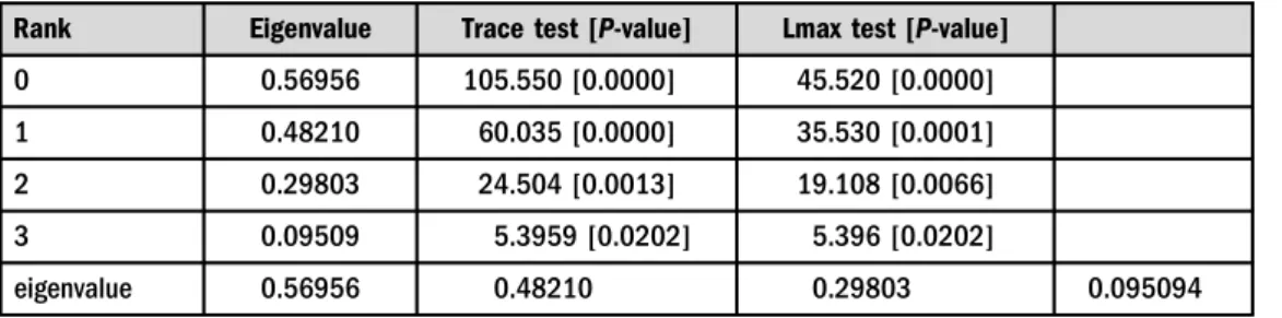
Results of the Johansen test (including trace and eigenvalue) show that at the significance level of 0.05 co-integration of order one occurs (Table 6).

Due to the occurrence of unit element in all-time series and the existence of cointegration between model variables, it was possible to extend and transform the model into vector error correction models.

6. VECM MODEL AND EMPIRICAL RESULTS

Verification of co-integration was carried out with the use of the Engle-Granger and Johansen test which confirmed the occurrence of co-integration, and thus, justified the use of the VECM model for the lag order 4 and co-integration of order 1.

In accordance with the Granger representation theorem, if variablesy_tandx_tare integrated of order I(1) and are co-integrated, the relationship between them can be represented as a vector error correction model (VECM) (Piłatowska 2003).

Table 5.Results of the Engle–Granger co-integration test

Specification d_GDP d_EQ d_ RoE d_DI

Unit root appears a51; I(1) a51; I(1) a51; I(1) a51; I(1) τe(asymptoticP-

value)

2.6194 (0.08896)

6.1443 (5.343e 008)

3.8899 (0.00212)

5.1379 (1.057e 005)

Note: ADF test with constant, test statistic tau_c(1)τe(asymptoticP-value), lag order54.

Source: Author’s own calculations.

Table 6.Johansen test

Rank Eigenvalue Trace test [P-value] Lmax test [P-value]

0 0.56956 105.550 [0.0000] 45.520 [0.0000]

1 0.48210 60.035 [0.0000] 35.530 [0.0001]

2 0.29803 24.504 [0.0013] 19.108 [0.0066]

3 0.09509 5.3959 [0.0202] 5.396 [0.0202]

eigenvalue 0.56956 0.48210 0.29803 0.095094

Source: Author’s own calculations.

The general form of the VECM model can be written as:

ΔYt¼ G1ΔYt−1þG2ΔYt−2þ. . .þGk−1ΔYt−kþ1þpYt−kþ«t¼X^k−1

i¼1

GiΔYt−iþpYt−kþ«t;

(2) where

Gi¼ Xⁱ

j¼1

AjΙ; i¼1;2; . . .;k1; Gk¼p¼−pð1Þ ¼− ΙX^k

i¼1

Ai

!

and Ι is a unit matrix.

Analysis of the VECM model allows us to draw the following conclusions: the levels of vector f parameters indicating the rate of GDP adjustments in successive VECM model equations show that the highest rate of these adjustments was noted for own changes in GDP.

Some conclusions can be drawn from the evaluation of the vector correction model component (EC1) representing the mechanism of short-term adjustments which serves attainment of the long-term model balance. The evaluation of the EC1 indicates that the strongest correction of the deviation from long-term equilibrium occurs in the case of the DI equation.

Here, around 4.5% of the imbalance from the long-term growth path is corrected by a short- term adjustment process. Weaker deviation adjustments occur for GDP (2.12%), EQ (1.15%) and for RoE (0.12%). The values of the coefficient of determinationR²reveal adjustment of the VECM model equations to empirical data, i.e., for GDP (67.86%), EQ (66.57%), RoE (87.49%) and DI (93.11%) (Table 7).

Table 7. The main research results for VECM model (lag order54, rank51)

Maximum likelihood estimates, observations 2005:22019:4 (T559)

b(Cointegrating vectors) (standard errors) a(Adjustment vectors)

d_GDP 1.0000 (0.00000) d_GDP 0.021222

d_EQ 16.825 (6.7557) d_EQ 0.011570

d_RoE 44.967 (14.841) d_RoE 0.0012407

d_DI 72.791 (10.988) d_DI 0.044618

Specification d_d_GDP d_d_EQ d_d_RoE d_d_DI

Coefficient (P-value)

EC1 0.0212 (0.5289) 0,0116 (0.3615) 0.0012 (0,8379) 0,0446 (8.23e09)

R2 0.678619 0.665721 0.874899 0.931127

DW 1.927042 2.082761 2.260048 2.080093

Source: Author’s own calculations.

In order to verify the correctness of the VECM model results two tests were carried out verifying the occurrence of autocorrelation, i.e.: Autocorrelation Ljung-Box Q⁰test, lag order for test54 and ARCH test, lag order for test 54.

Ljung-Box tests (LMF, LM, Q) were carried out to verify autocorrelation, for the lag order 4.

The verifying statistic using the autocorrelation coefficient function (ACF) in the form Q⁰and empiricalP-value levels higher than the nominal onef 50.05, let us conclude that there is no autocorrelation in the residual process (Kufel 2011: 110111).

The ARCH test results indicate that in the examined model of the residual-based process (four variables), the ARCH effect is not observed because LM test statistics are lower than the levels ofc². This means that there is no autoregressive changeability of the conditional variance and there is no need to estimate model parameters by means of weighted least squares method.

Thus, the results of both tests which were carried out, confirm credibility of the VECM model and allow us to draw conclusions on their basis.

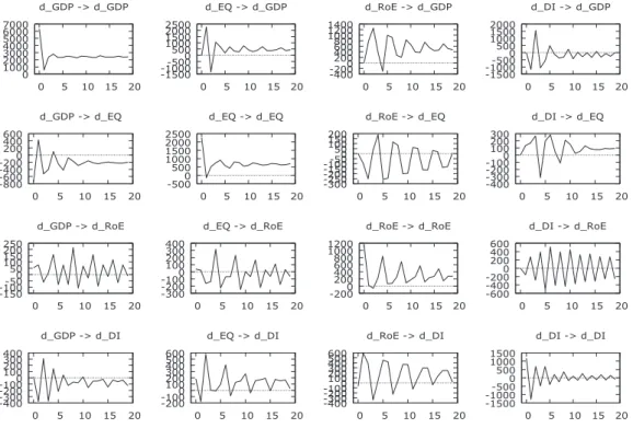
6.1. The impulse response functions

Analysis of the GDP responses to shocks derived from FDI components reveal that the GDP responses are the strongest to impulses from EQ and RoE. The impact of debt instruments, affects GDP changes comparably less. The summary list of all impulses and answers is shown inFig. 4.

1000 0 2000 3000 4000 5000 6000 7000

0 5 10 15 20 d_GDP -> d_GDP

-1500 -1000 1000 1500 2000 2500-500 500 0

0 5 10 15 20 d_EQ -> d_GDP

-400-200 200 400 600 800 0 1000 1200 1400

0 5 10 15 20 d_RoE -> d_GDP

-1500 -1000 1000 1500 2000-500 500 0

0 5 10 15 20 d_DI -> d_GDP

-800-600 -400-200 0 200 400 600

0 5 10 15 20 d_GDP -> d_EQ

-500 500 0 1000 1500 2000 2500

0 5 10 15 20 d_EQ -> d_EQ

-300-250 -200-150 -100-50 50 0 100 150 200

0 5 10 15 20 d_RoE -> d_EQ

-400-300 -200-100 100 200 300 0

0 5 10 15 20 d_DI -> d_EQ

-150-100-50 50 0 100 150 200 250

0 5 10 15 20 d_GDP -> d_RoE

-300-200 -100 100 200 300 400 0

0 5 10 15 20 d_EQ -> d_RoE

-200 200 400 600 800 0 1000 1200

0 5 10 15 20 d_RoE -> d_RoE

-600-400 -200 200 400 600 0

0 5 10 15 20 d_DI -> d_RoE

-400-300 -200-100 0 100 200 300 400

0 5 10 15 20 d_GDP -> d_DI

-200-100 100 200 300 400 500 600 0

0 5 10 15 20 d_EQ -> d_DI

-400-300 -200-100 0 100 200 300 400 500 600

0 5 10 15 20 d_RoE -> d_DI

-1500 -1000 1000 1500-500 500 0

0 5 10 15 20 d_DI -> d_DI

Source: Author’s own calculations.

Fig. 4.Impulse response function –for horizon period 20 quarters

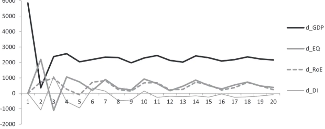
The strongest GDP responses occur in periods (quarters): 1^st, and next 3^rd-4^thshowing sta- bilisation in subsequent periods. Periods 3 and 4 are characterised by a falling tendency after which fluctuations in GDP responses stabilise slowly, usually from period 5 or 6. The GDP responses to their own errors in forecasts, indicate fading/weakening tendencies in periods 1–3, to stabilise in successive periods and clearly from period 20 onwards. However, presentation of GDP responses to impulses shows clearly that GDP responds most strongly to its own standard deviations (Fig. 5).

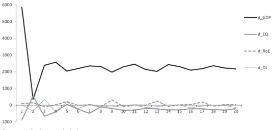
While the components of FDI responses to impulses of GDP remain mainly positive in the case of RoE, very weaker for equity and become negative for debt instruments. The debt in- strument responses reach the maximum positive value in period 3. All examined FDI compo- nents to GDP-derived impulses show clearly that they demonstrate weakening tendencies in the initial periods (1–2) (Fig. 6).

The research results for Poland are convergent with e.g., Polat (2017), who examined the relationships between RoE (i.e., one FDI component) and selected macroeconomic indicators for 80 countries in the period of 2006–2012. Her studies found strong evidence that RoE are positively correlated with political risk ratings (confidence level) and also with GDP, GDP growth rate and consumer confidence level in each host country and are negatively associated with repatriation and payment delay risk ratings.

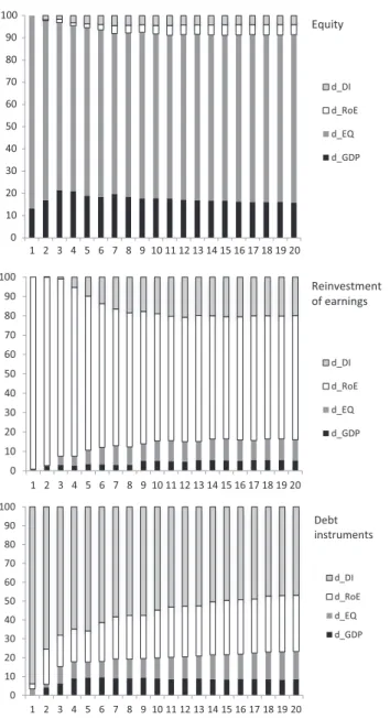
6.2. The decomposition of variance

Results of GDP decomposition indicate that in period 1 these changes are in 100% accounted for by their own forecast errors. In period 2, their own changes lose in significance (84.0%), and such FDI components as RoE (1.4%), equity (11.8%) and debt instruments (2.8%) grow in significance.

In the following periods, GDP’s own changes stabilise the constant effect at the level of 84.7%, whereas RoE grows (3.8%), and similarly, debt instruments grow (3.0%) and equity loses in sig- nificance (8.4%). Thus, we can conclude that FDI significance in forecasting the degree of explanation of GDP amounts jointly to ca. 15.2% in the 20^thquarter, it’s 5 years (Fig. 7).

-2000 -1000 0 1000 2000 3000 4000 5000 6000

1 2 3 4 5 6 7 8 9 10 11 12 13 14 15 16 17 18 19 20

d_GDP

d_EQ

d_RoE

d_DI

Source: Author’s own calculations.

Fig. 5.Response of GDP to a standard shock in own GDP and components of FDI inflows (quarters)

Results of decomposition for EQ show that the degree of its explanation in periods 1 and 20 of the forecast depends, first of all, on own forecast errors (86.7% and 75.2%, respectively) and when it comes to GDP–13.3% and 16.1%, respectively.

Next, results of the degree of explanation of changes in RoE indicate that in period 1 these changes are accounted for in 99.2% by own forecast errors, in 0.8% by GDP, 0.7% by equity and in 0.0% by debt instruments (DI). In period 20 of the forecast the degree of explanation of reinvestment is distributed almost evenly between: reinvestment own changes (63.4%) and debt instruments (20.1%), and also, equity (11.0%) and GDP (5.4%).

In the case of debt instruments (DI) the key significance in their explanation have own forecast errors (93.8% and 46.9%) and RoE (2.8% and 29.9%), and especially, in period 20 GDP (0.0% and 8.6%) (Fig. 8).

-1000 0 1000 2000 3000 4000 5000 6000

1 2 3 4 5 6 7 8 9 10 11 12 13 14 15 16 17 18 19 20

d_GDP

d_EQ

d_RoE

d_DI

Source: Author’s own calculations.

Fig. 6.Responses of FDI to a one-standard error shock in d_GDP (quarters)

0 10 20 30 40 50 60 70 80 90 100

1 2 3 4 5 6 7 8 9 10 11 12 13 14 15 16 17 18 19 20 d_DI d_RoE d_EQ d_GDP GDP

Source: Author’s own calculations.

Fig. 7.Forecast variance decomposition for GDP (quarters)

A detailed analysis of the decomposition of the analysed variables from the 1^stto the 20^th quarter of the forecast variables indicate that the strongest impact (apart from their own forecast errors) was as follows for:

0 10 20 30 40 50 60 70 80 90 100

1 2 3 4 5 6 7 8 9 10 11 12 13 14 15 16 17 18 19 20

0 10 20 30 40 50 60 70 80 90 100

1 2 3 4 5 6 7 8 9 10 11 12 13 14 15 16 17 18 19 20 d_DI d_RoE d_EQ d_GDP d_DI d_RoE d_EQ d_GDP

Reinvestment Equity

of earnings

0 10 20 30 40 50 60 70 80 90 100

1 2 3 4 5 6 7 8 9 10 11 12 13 14 15 16 17 18 19 20 d_DI d_RoE d_EQ d_GDP Debt instruments

Source: Author’s own calculations.

Fig. 8.Forecast variance decomposition for EQ, RoE and DI (quarters)

GDP–12.4% EQ (Q4), 3.9% RoE (Q19) and 5.6% DI (Q5), RoE–5.5% GDP (Q17), 10.9% EQ (Q19) and 20.5% DI (Q16).

Moreover, we can add that the results obtained for the GDP decomposition of variance are convergent, for example, with the research results achieved byKosztowniak (2016)in the field of GDP decomposition with participation of FDI (jointly for all components) in her studies for Poland in the years of 1992–2012. Her investigations indicated that FDI accounted for GDP changes in 1.7% in period 2 and this value increased to 5.23% in period 10 of the forecast. This means confirmation of the presented research results and maintaining growing degrees of explanation for GDP changes by FDI components, in the consecutive years of the study, i.e. 2004: Q12019: Q4. Jointly, the degree of explanation of GDP by the above mentioned FDI financial instruments amounts to approx. 15.2% in the 20^th quarter.

This increase in the explanation of GDP changes results from the growth of FDI inward stocks, maintaining current investments (increase in RoE) and the inflow of new investments (increase in equity).

According to the 2019Eurostat data in the European Union between 2010 and 2016, the share of value added by foreign-controlled enterprises rose by 2.3%. At the level of the individual EU member states, the countries with the highest shares of value added by foreign-controlled enterprises in 2016 were Hungary (51.4%), Slovakia (48.1), Luxembourg (44.6%) and Poland (36.8%). In contrast, four EU member states had shares under 20%: Cyprus (13.4%), Italy (15.8%), Greece (16.3%) and France (16.4%) compared to the average for EU-26 (25%).

7. CONCLUSIONS

The aim of this paper is to analyse the cause-and-effect relationships between RoE and other components of FDI inflows and GDP in Poland in the years of 2004–2019. The modelling results of VAR/VECM, the impulse response functions and forecast error variance decompo- sition analysis confirmed the occurrence of mutual dependencies.

We stated that:

1. Changes in the structure of FDI in Poland during 2004–2019 were adequate to the theoretical cycle of FDI life. The increase in RoE results from the implementation of the 2^nd stage in most foreign investments.

2. The increase in the share of RoE in the structure of FDI inflows accompanied a decrease in shares and other forms of equity participation. In the analysis years of 1994–2019, the share of capital in the structure of the FDI inflows decreased from ca. 60%–15% and debt in- struments with ca. 20%–5%, with the increase in the share of RoE from 20% to 80%.

3. The increase in the share of reinvestment of earnings in the structure of FDI inflows accompanied by the increase in the impact of these investments on changes in GDP.

GDP decomposition analysis indicates that the current GDP changes to the largest extent are explained by forecast: own errors from 100% in the 1^stperiod to 84.7% in the 20^thperiod, and from 2^ndperiod to 20^thperiod–in case of equity from 11.9% to 8.4%, RoE from 1.3% to 3.8%

and debt instruments from 2.8% to 3.0%.

Jointly, the degree of explanation of GDP by the above mentioned FDI financial instruments amounts to ca. 15.9% (2^ndperiod) and 15.2% (20^thperiod). That is, the importance of equity

decreases with other FDI components. Although the total degree of explanation of changes in GDP by FDI changes remains comparable.

Our research results allowed to positively verify the hypothesis that the changes in the structure of FDI inflows in Poland are in line with the phases of the FDI life cycle. The increase in the share of RoE in the structure of these investments is also accompanied by an increase in the impact and the degree of explanation of changes in GDP.

Summing up, the effectiveness of the impact of FDI inflows on GDP is determined not only by the value of FDI inflows but also by the changes in their financial structure. Changes in the strength of individual FDI components for GDP in Poland will increase in the future, which is related to the stages of the FDI life cycle and the stages of economic development.

Considering the positive impact of RoE on changes in GDP has been demonstrated– the government and specialised agencies e.g., Polish Investment & Trade Agency should strengthen the investment incentives for foreign investors who decide to maintain FDI, including as part of the increase in the RoE. Particularly important for Poland as an FDI host country is the consolidation of the reinvestment process in industries supporting competitiveness and inno- vation as well as creating the highest added value.

REFERENCES

Acaravci, A.– Ozturk, I. (2012): Foreign Direct Investment, Export and Economic Growth: Empirical Evidence from New EU Countries.Romanian Journal of Economic Forecasting, 2.

Alfaro, L.–Chanda, A.–Kalemli-Ozcan, S.–Sayek, S. (2001): FDI and Economic Growth: The Role of Local Financial Markets. Harvard Business School,Working Paper, No. 01-083.

Bacic, K.–Racic, K.–Ahec-Sonje, A. (2005):The Effects of FDI on Recipient Countries in Central and Eastern Europe.Hamburg Institute of International Economics.

Balasubramanyam, V. N.–Salisu, M.–Sapsford, D. (1996): Foreign Direct Investment as an Engine of Growth.Journal of International Trade and Economic Development, 8(1): 27–40.

Bende-Nabende, A.–Ford, J. L.–Sen, S.–Slater, J. (2000):Long-Run Dynamics of FDI and its Spillovers onto Output: Evidence from the Asia-Pacific Economic Cooperation Region. University of Birmingham Department of Economics,Discussion Paper, No. 00-10.

Blomstr€om, M. (1986): Foreign Direct Investment and Productive Efficiency: The Case of Mexico.Journal of Industrial Economics, 15(1): 97–110.

Brada, J. C.–Tomsık, V. (2003): Reinvested Earnings Bias, the‘Five Percent’Rule and the Interpretation of the Balance of Payments–with an Application to Transition Economies. William Davidson Institute, Working Paper, No. 543.

Carkovic, M.–Levine, R. (2002): Does Foreign Direct Investment Accelerate Economic Growth. University of Minnesota, Department of Finance,Working Paper.

Carkovic, M. – Levine, R. (2005): Does Foreign Direct Investment Accelerate Economic Growth? In:

Moran, T.–Graham, E.–Blomstr€om, M. (eds):Does Foreign Direct Investment Promote Development?

Washington, DC: Institute for International Economics, pp. 195–220.

Chowdhury, A.–Mavrotas, G. (2005): FDI and Growth: A Causal Relationship. United Nations University, WIDER,Research Paper, No. 25.

Damgaard, M. L.–Laursen, F.–Wederinck, R. (2010): Forecasting Direct Investment Equity Income for the Danish Balance Payments. Denmark National Bank,Working Papers, No. 65.

Edwards, A.–Todd, K.–Ryan, J. (2014): Trapped Cash and Profitability of Foreign Acquisitions.Rotman School of Management Working Paper, No. 1983292: 1–50.

Ericsson, J.–Irandoust, M. (2001): On the Causality Between Foreign Direct Investment and Output: A Comparative Study.The International Trade Journal, 15(1): 122–132.

Eurostat (2019):Foreign-Controlled Enterprises in EU: Value Added,Https://Ec.Europa.Eu/Eurostat/Web/

Products-Eurostat-News/-/DDN-20190411-1 (11.04.2019).

Fajgelbaum, P.–Grossman, G. M.– Helpman, E. (2015): A Linder Hypothesis for Foreign Direct In- vestment.Review of Economic Studies, 82: 83–121.

Ghebrihiwet, N. (2017): Acquisition or Direct Entry, Technology Transfer, and FDI Policy Liberalization.

International Review of Economics & Finance, 51(2): 455–469.

Gorynia, M.–Nowak, J.–Wolniak, R. (2005):Fostering Competitiveness of Polish Firms: Some Musings on Economic Policy and Spatial Expansion. International Management Development Association, XIV, pp. 428–435.

Gorynia, M.–Nowak, J.–Wolniak, R. (2011): Investing in a Transition Economy. Motives and Modes of Foreign Direct Investment in Poland. In: Marinov, M.–Marinova, S.:The Changing Nature of Doing Business in Transition Economies.Palgrave Macmillan, pp. 148–182.

Gorynia, M.– Nowak, J. – Tra¸pczynski, P. –Wolniak, R. (2015): Government Support Measures for Outward FDI: An Emerging Economy’s Perspective.Argumenta Oeconomica, 1(34): 229–258.

Gurgul, H.–Lach,Ł. (2009): Zwia¸zki Przyczynowe Pomie¸dzy Bezposrednimi Inwestycjami Zagranicznymi W Polsce a Podstawowymi Wskazniki Makroekonomiczne (Wyniki Badan Empirycznych) (Causalities Between Foreign Direct Investment in Poland and Basic Macroeconomic Indicators (Empirical Find- ings)).Ekonomia Menadzerska, 6: 77–91._

Herzer, D. – Klasen, S. – Howak-Lehmann, F. (2008): In Search of FDI-Led Growth in Developing Countries: The Way Forward.Economic Modelling, 25(5): 793–810.

Jarosinski, M. – Barło_zewski, K. (2019): Differences in Competitive Strategies between Rapidly and Incrementally Internationalising Firms.Acta Oeconomica, 69(S2): 161–187.

Johansen, S. (1995): Likelihood-Based Inference in Cointegrated Vector Autoregressive Models. Oxford:

Oxford University Press.

Kang, Y.–Du, J. (2005):Foreign Direct Investment and Growth: Empirical Analyses on Twenty OECD Countries.Http://Www.Ssc.Uwo.Ca/Economics/Undergraduate/400E-001/Draftpapers/Dukang.Pdf.

Knetsch, T. A.–Nagengast, A. J. (2016): On the Dynamics of the Investment Income Balance. Deutsche Bundesbank,Discussion Paper, No. 21: 1–36.

Kornecki, L.–Raghavan, V. (2011): Inward FDI Stock and Growth in Central and Eastern Europe.The International Trade Journal, 25(5): 539–557.

Kosztowniak, A. (2016): Verification of the Relationship Between FDI and GDP in Poland.Acta Oeco- nomica, 66(2): 307–332.

Kufel, T. (2011):Ekonometria (Econometrics). Warsaw: Wydawnictwo Naukowe PWN.

Lin, M.–Kwan, Y. K. (2016): FDI Technology Spillovers, Geography, and Spatial Diffusion.International Review of Economics&Finance, 43: 257–274.

Liu, X.–Siler, P.–Wang, Ch.–Wei, Y. (2000): Productivity Spillovers from Foreign Direct Investment:

Evidence from UK Industry Level Panel Data. Journal of International Business Studies, 31(3):

407–425.

Lundan, S. M. (2006): Reinvested Earnings as a Component of FDI: An Analytical Review of the De- terminants of Reinvestment.UN Transnational Corporations, 15(3): 33–64.

Marona, B. – Bieniek, A. (2013): Wykorzystanie Modelu VECM do Analizy Wpływu Bezposrednich Inwestycji Zagranicznych na Gospodarke¸ Polski w Latach 1996–2010 (Analysis of the Influence of Foreign Direct Investment on Polish Economy in 1996–2010 Using VECM Methodology).Acta Uni- versitatis Nicolai Copernici–Ekonomia, XLIV(2): 333–350.

Mencinger, J. (2003): Does Foreign Direct Investment Always Enhance Economic Growth?International Review for Social Sciences, Kyklos, 56(4): 491–509.

Misztal, P. (2012): Bezposrednie Inwestycje Zagraniczne Jako Czynnik Wzrostu Gospodarczego w Polsce (Foreign Direct Investment as a Factor of Economic Growth in Poland).Finanse, 1(5): 9–26.

Molendowski, E. –Polan, W. (2013): Changes in Intra-Industry Competitiveness of the New Member States (EU-10) Economies during the Crisis, the Years 2009–2011.Comparative Economic Research, 16:

63–83.

NBP (2017):Balance of Payments Statistics. Methodological Notes. Department of Statistics NBP, Warsawa.

NBP (2020):Balance of Payments, Financial Account–Direct Investment, 2020.

Novotny, F. (2015): Profitability Life Cycle of Foreign Direct Investment and its Application to the Czech Republic. Czech National Bank,Working Paper Series, No. 11: 1–25.

Novotny, F. (2018): Profitability Life Cycle of Foreign Direct Investment: Application to the Czech Re- public.Emerging Markets Finance and Trade, 54(7): 1623–1634.

Novotny, F.–Podpiera, J. (2008): The Profitability Life-Cycle of Direct Investment: An International Panel Study.Economic Change and Restructuring, 41(2): 143–153.

Nunnenkamp, P.–Schweickert, R.–Wiebelt, M. (2007): Distributional Effects of FDI: How the Interaction of FDI and Economic Growth Policy Effects Poor Households in Bolivia.Development Policy Review, 25(4): 429–450.

OECD (2018): Benchmark Definition of Foreign Direct Investment. Fourth Edition. Paris: OECD Pub- lishing, pp. 70–72.

OECD (2020): OECD Stat., International Trade and Balance of Payments,https://stats.oecd.org.

Oseghale, B. D. – Nwachukwu, O. C. (2010): Effect of the Quality of Host Country Institutions on Reinvestment by United States Multinationals: A Panel Data Analysis.International Journal of Man- agement, 27(3): 497–510.

Piłatowska, M. (2003):Modelowanie Niestacjonarnych Procesow Ekonomicznych. Studium Metodologiczne (Modelling of Non-Stationary Economics Processes. A Methodological Study). Uniwersytet M. Koper- nika, Torun.

Polat, B. (2017): Determinants of Reinvested Earning as a Component of Foreign Direct Investment.

Journal of Economics and Management Research, 6(1): 24–45.

Salorio, E. M.–Brewer, T. L. (2013): Components of Foreign Direct Investment Flows.Latin American Business Review, 1(2): 27–45.

Saltz, I. (1992): The Negative Correlation between Foreign Direct Investment and Economic Growth in the Third World: Theory and Evidence.Rivista Internazionale di Scienze Economiche e Commerciali, 39:

617–633.

Shultz, T. – Fogarty, T. (2009): The Fleeting Nature of Permanent Reinvestment: Accounting for the Undistributed Earnings of Foreign Subsidiaries.Advances in Accounting, 26(1): 112–123.

Supriyadi, D.–Satria, D. (2017): Model of Causality between FDI and Gross Domestic Product on ASEAN- 5 Countries from 1980–2014.Journal of Indonesian Applied Economics, 7(1): 1–17.

Szabo, S. (2019):FDI in the Czech Republic: A Visegrad Comparison. Economic Brief 042, Luxembourg, European Commission.

Taylor, T.–Mahabir, R.–Jagessar, V.–Cotton, J. (2013):Examining Reinvestment in Trinidad and Tobago.

Central Bank of Trinidad and Tobago, Port-of-Spain,Working Paper, No. 10.

Toda, H. Y.–Yamamoto, T. (1995): Statistical Inference in Vector Autoregressions with Possibly Inte- grated Processes.Journal of Econometrics, 66(1-2): 225–250.

Yamada, H.–Toda, H.Y. (1998): Inference in Possibly Integrated Vector Autoregressive Models: Some Finite Sample Evidence.Journal of Econometrics, 86(1): 55–95.