.
Research Article
© 2018 Kiss Gabor David and Isaac Kwesi Ampah.
This is an open access article licensed under the Creative Commons Attribution-NonCommercial-NoDerivs License (http://creativecommons.org/licenses/by-nc-nd/3.0/).
Macroeconomic Volatility and Capital Flights in Sub-Saharan Africa:
A Dynamic Panel Estimation of some Selected HIPC Countries
Kiss Gabor DavidUniversity of Szeged, Faculty of Economics and Business Administration, H-6722 Szeged, Kálvária Sgt 1. Hungary
Isaac Kwesi Ampah
University of Szeged, Faculty of Economics and Business Administration,
H-6722 Szeged, Kálvária Sgt 1. Hungary Doi: 10.2478/mjss-2018-0148
Abstract
For several years, illicit financial outflows though unobservable have remained rampant in the sub- Saharan Africa (SSA) sub-region. This paper examines whether macroeconomic volatilities as perceived by domestic investors in the sub-region have any influence on these outflows taking some selected Heavily Indebted Poor Countries (HIPC) and dataset for the period 1990 to 2012 as the case study. In addition, the study employs a Generalized Autoregression Heteroscedasticity (GARCH) model and Panel Autoregressive Distributed Lag model in its estimation. The outcomes of the econometric investigation, which reflects the current situation in the sub-region, support the view that domestic investors will withdraw their investments and other financial holdings from the domestic economy if they perceived present and future government policies to be volatile. These results suggest that government in HIPC Countries in SSA should focus on stabilising their macroeconomic and political situation if they want to reduce the outflow of domestic capital.
Keywords: sub-Saharan Africa; Capital Flight; Heavily Indebted Poor Countries; Generalized Autoregression Heteroscedasticity; Pooled Mean Group (PMG).
Introduction 1.
Over the past forty years (1970 to 2010), sub-Saharan Africa (SSA) countries alone have lost more than $814.2 billion with compound interest reaching over $1.06 trillion - draining valuable national resources that could have been used for building infrastructure and capital investment, facilitating the underground economy, worsening the income inequality, and promoting crime and corruption in the sub-region. Interestingly, this amount exceeds the combined economic size of these countries as indicated by their Gross Domestic Product ($1.05 trillion), official development aid of $659.5 billion and $306.4 billion of Foreign Direct Investment for the same period (Boyce and Ndikumana, 2012). According to the UN-Economic Commission for Africa (2015), these estimates might even fall below the actual values since accurate statistics for the computation of illicit financial flows do not exist for some countries, and, may also exclude other form of capital outflow that by nature are difficult to measure such as proceeds from drug or human trafficking and/or corruption.
These outflows of resources are of serious concern, given the low level of development and the extreme nature of poverty in the region. Currently, access to good quality healthcare, safe and
potable water, proper education and housing are limited in the sub-region. The number of the sub- regions population is living less than US$1.25 a day is still predicted to have increased by more than 100 million [from 290 million in 1990 to 414 million in 2010 (UN-Economic Commission for Africa, 2015)]. What is more disturbing is the steady rise in commodity and fuel prices and the massive reductions of official development assistance and foreign direct investment in the region after the global economic and financial crises. These reasons coupled with the balance of payment difficulties of most countries in the region have called for the need for more resource mobilisation either locally or abroad to achieve the Sustainable Development Goals (SDG’s) the sub-region envisages.
A study by Atisophon et al. (2011) indicates that SSA would need an extra capital of about
$72 billion to $89 billion per year to achieve the economic growth rates that are compatible with the Millennium Development Goals (MDG’s) at that time. At the sectoral level, Nkurunziza (2014) also added that Africa would need to invest about $93 billion a year in building new infrastructure and in the maintenance of existing infrastructure for ten years in addition to $54 billion in developing small- scale and large-scale irrigation. The main question is if resources are that relevant to the growth and development of the sub-region, then what are the factors driving these resources out. The literature indicates that if the content and direction of present and future macroeconomic policies are uncertain and/or volatile, domestic investors will be unsure about the effect of these macroeconomic volatilities on the value of their assets locally. This vulnerability may motivate them to pull back their investments from the economy and invest in foreign assets instead. In this paper, we investigate this issue and examine whether domestic macroeconomic uncertainties in the region have any influence on the growing capital flight.
Apart from the introduction which also specifies the aim of the research, the rest of the paper is structured as follows. Section two presents overview of how capital flight and macroeconomic volatility are defined and measured in the literature, as well as a review of the recent theoretical and empirical literature whereas the methodological framework, data sources and estimation techniques employed in the study, are also analysed critically in section three. Section four and five examines and discusses the results, the conclusion as well as the policy implications of the paper.
Literature Review 2.
The determinants of capital flight in the SSA have been an attractive area of research, both theoretically and empirically. However, before sharing some of these studies, this paper provides a review of the definition and measurement of capital flight and volatility in the literature.
2.1 Definition and measurement of capital flight
The notion of capital flight means different things to different people and even different things to the same person. Sometimes, it is seen as legal since the capital outflows, and the sources of funds are considered legitimate. While at the other end, capital flight is considered illegal since capital outflows representing the transfer abroad are out of reach of domestic law enforcement and tax authorities. For instance, capital outflows from developed countries are often referred to as an outward foreign direct investment (OFDI), while, such outflows from developing countries are labelled as capital flight. As a result, there are conflicting views on the definition of capital flight in the literature, and this has generated different definitions with different meanings. Loosely defined, capital flight is the unreported private accumulation of foreign assets (Eggerstedt et al. 1995).
Trevelline (1999) defined capital flight as any cross-border transfer of money where the transfer is motivated either by the desire to flee a weak currency’s limited investment opportunities or the desire to secret money away from government authority. Deppler and Williamson (1987) define it as the acquisition or retention of a claim on non-residents, motivated by the owner’s concern that the value of his/her assets would be subject to discrete losses or impairment if his/her claims continued to be held domestically. This study interprets capital flight as consisting of private capital outflows of any kind, motivated by the residents’ (of any country) desire to reduce the actual and potential level of government control (including the risk of expropriation) over such capital and as well to acquire
foreign assets.
Just like the definition of the term, capital flight measurement has followed a similar trend.
There are several approaches used in the literature to measures capital flight. The residual method used by World Bank in 1985 and further modified by Morgan Guaranty Trust in 1986, the Hot money measure or balance of payment method introduced by Cuddington’s (1986), the Mirror stock statistics or the asset method by Collier et al., (2001). The Dooley’s method which includes all capital outflows placed beyond the control of domestic authorities was also utilised by Dooley in 1986 and later Deppler and Williamson (1987). In this paper, capital flight is measured by employing the methodology outlined by Ndikumana, Boyce and Ndiaye (2014) which is a modified version of the World Bank (1985) residual method. This method computes capital flight as the variation between recorded capital inflows and foreign-exchange outflows. Adjustments are made for trade misinvoicing, under-reporting of remittances, inflation and exchange rate. Capital flight is therefore estimated as
CF = 𝛥DEBTADJ + FDI – (CA +𝛥RES) + MISIN + RID
Where: CF represent capital flight, 𝛥DEBTADJ is the change in the stock of external debt outstanding adjusted for exchange rate fluctuations, FDI is a net foreign direct investment, 𝛥RES represents net additions to the total stock of external reserves, CA is the current account deficit, MISIN is the net trade misinvoicing and RID represent unrecorded remittances. Ndikumana, Boyce and Ndiaye (2014) presented a detailed analysis of how these indicators where measured.
2.2 Definition and measurement of macroeconomic volatility
Logically, it is not too difficult to accept the notion that the general macroeconomy, whether stable or volatile can have an influence on the flow of capital in a country but modelling it can be very challenging primarily due to its multiplicity of causes or multidimensional phenomenon. In a simpler form, Frenkel and Goldstein (1991) defined volatility of a variable as representing short-term variations of a variable from their longer-term trends. In this way, volatility reflects a situation where a variable say GDP per capita assume values far different from its mean value. In mainstream economics, such variations in a series is not necessarily a problem. We realised that economic agents such as government, firms or individual consumers always act or make decisions without knowing the actual values of the inputs at the time of the decision making. Therefore, they do so by making certain assumptions about the behaviour of the variables and assign a probability to their various states. This decision is almost always subjected to cyclical and seasonal variations.
According to Abaidoo (2012), the fluctuations in economic decisions become more problematic when they are large and can not be predicted, generating uncertainty for consumers, manufacturers, government officials or investors. To him, decision making under this kind of volatility can either lead to a bad decision or suboptimal decisions for these economic agents.
For the purpose of this study, we defined macroeconomic volatility as large fluctuations of an economic variable arising from domestic or external shocks that are unforeseen or unpredictable.
Since volatility is not predictable or even observable, it is not easy to quantify it. In the literature, what most of the empirical studies does is to compute the mean of a variable and examine the variation of the variable from its mean. If the variation of the variable is greater than fifty (50) percent (%) or close to 100% then clearly uncertainty does exits in the variable. This study shall use the recently developed ARCH and GARCH model introduced by Bollerslev (1986), and Taylor (1986) in computing the conditional variance of the macroeconomic variables considered.
2.3 Determinants of capital flight
Studies examining the determinants of capital flight in the SSA region can be divided into two main groups. The first group based its investigation on the portfolio theory of international capital flows where capital flight is seen as an outcome of portfolio choice by economic agents as they choose between domestic and foreign assets to allocate their wealth to maximize the overall risk-adjusted
return on their portfolios (Fofack and Ndikumana, 2014; Collier et al., 2001; Cuddington, 1987). In this context, the impact of domestic macroeconomic variables on the relative returns between domestic and foreign assets are seen as the main cause of capital flight. For instance, factors such as large interest rate differentials, overvalued exchange or more specifically the expected rate of appreciation or depreciation of the exchange rate; and other determinants of the rate of return to investment are found to be the main driver of capital flight.
The second group of studies also based on the "risk differentials" approach where capital flight is based on the differences in the perceived risks associated with investing domestically or abroad.
Factors such as inflation inconsistency and unsustainable fiscal and monetary policies; volatile regulatory environment and the legal system etc. are the causes of capital flight. Unfortunately, this second approach which serves as the focus of this study has not been an attractive area of research for some time now. Empirical studies have only been interested in examining the impact of domestic policies on capital flight and not the risk part which represents the volatility. Table 1 provides brief sample evidence of the current studies conducted in examining the determinants of capital flight in the SSA sub-region.
Table 1: Sample empirical evidence of the determinants of capital flight in SSA
Source: compiled by the authors
Author(s) Nature of examination Country Time
frame Estimation
Technique Major Finding(s)
Ndikumana
(2016) Causes and Effects of capital flight
Africa (Cameroon, Congo, Zimbabwe, Kenya, and Ethiopia, Burkina Faso and Madagascar
1990-
2012 Case studies Mixed results
Mucha – Muchai
(2016) Fiscal policy and capital
flight Kenya 1970–
2012 ARDL taxation and
government expenditure policies
Ramiandrisoa – Rakotomanana (2016)
Why is there capital flight
from developing countries Madagascar 1970–
2012 Vector Auto
Regressive (VAR) political and macroeconomic crises
Domfeh (2015) capital flight and institutional
governance 32 sub-Saharan African
countries 2000-
2012
Generalized Method of Moments (GMM),
Fixed Effect and the pooled-OLS regression models
macroeconomic uncertainty, institutional and political instability, less developed financial system, and higher interest rate differentials Salisu – Isah (2017
Capital Flight-Growth Nexus in Sub-Saharan Africa: The Role of Macroeconomic Uncertainty
28 Sub-Saharan African
countries 1986 –
2010
mean-group (MG) and pooled mean- group (PMG) estimators
macroeconomic uncertainty Osei-Assibey,
Domfeh – Danquah (2018)
Corruption, institutions and
capital flight: 32 sub-Saharan African
countries 2000-
2012
Generalized Method of Moment and Fixed Effect Regression
regime durability and the rule of law Ndikumana –
Boyce (2011) external debt and capital
flight Sub-Saharan African
Countries
1970 to 2008
GMM, Fixed Effect
and Random EffectExternal Debt
Hermes – Lensink (2001)
Capital flight and the uncertainty of government
policies Least Developed
Countries (LDCs) 1971–
1991
Generalized Method of Moments (GMM)
the uncertainty of budget deficits, tax payments, government consumption and the inflation rate Agu (2010) Domestic Macroeconomic
Policies and Capital Flight Nigeria Macro-econometric
Modelling Political risk and macroeconomic volatility
Model Specification
3.
To examine whether the uncertainties surrounding current and future direction of macroeconomic policies have any impact on illicit capital outflows in SSA, this paper draws on a similar model by Ampah et al. (2018), and Hermes and Lensink (2001) and estimate a dynamic panel data model where capital flight is a function of macroeconomic volatilities and other control variables as;
Where CF is capital flight, F represents domestic policies uncertainties, Z is a vector of other control variables and is the error term. β, and are the coefficients of CF, F and Z respectively. This study considers inflation rate volatility, political regime volatility, real interest rate volatility, and exchange rate volatility as the domestic macroeconomic volatility. Also, financial development (FD), Gross Domestic Product (GDP) and external debt (EXT) are also chosen as the control variables for the study. These variables are chosen as a result of carefully examining the theoretical and empirical literature. Therefore F and Z can be re-written as
Where VINF is inflation rate volatility; VREA is the real interest rate volatility, VPOL is the political stability volatility, and VEXC is the real exchange rate volatility. GDP also represent annual Gross Domestic Product per capita growth, EXT is total external debt as a percentage of GDP and FD is measured as a broad money supply (M2) as a percentage of GDP. Replacing equation (2) and (3) into equation (1) and specifying an extended form of the equation, the empirical model of the study can be re-written as;
Where are the parameters to be estimated? accounts for the stochastic error term and denotes the unobserved country-specific time-invariant effect. stand for a country, and is time. also, represent the constant All other variables are already defined. Table 2 provides a brief illustration of how the variables are defined and measured as well as their sources.
In estimating the volatility variables, this paper employs the Generalized Autoregressive Conditional Heteroskedasticity (GARCH) (1,1) models introduced by Bollerslev (1986), and Taylor (1986) to predict the time-varying conditional variance of the variables as a function of its past values. The choice of the GARCH (1,1) is based on the annual series nature of the data which tends to follow or support the GARCH process better. Also, because GARCH models are easy to apply and possess the ability to check the robustness of the model. Considering this, the GARCH (1,1) for the study is therefore defined as
Where
The conditional variance ( ) specified in equation (6), captures the mean ( ) of the conditional variance, data about previous volatility measured as the lag of the squared residuals from the mean equation ( ) which also it the Autoregressive Conditional Heteroskedasticity (ARCH) term and the previous forecast error variance, ( ) which is the GARCH term.
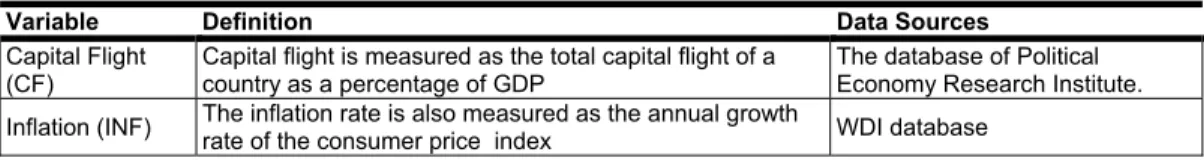
Table 2: Variables in the model: Measurements and data sources.
Variable Definition Data Sources
Capital Flight (CF)
Capital flight is measured as the total capital flight of a country as a percentage of GDP
The database of Political Economy Research Institute.
Inflation (INF) The inflation rate is also measured as the annual growth
rate of the consumer price index WDI database
0 1 1 2 3 (1)
it it it it it
C F =α + β C F − +δ F + ∂ Z +ε
ε
δ ∂( , , , ) (2)
F = f VIN F VPO L V REA VE XC
( , , ) (3) Z = f G D P EXT FD
1 1 1 2 3 4 5 6 7 8 (4)
it it it it it it it it i it
CF = +α βCF− +βVINF +βVPOL +βVREA +βVEXC +βGDP+βEXT +βFD u+ +ε
0 to 8
β β εit
ui i t
α1
1 (5)
it it it
vol = + ∂ϕ vol− +u (0, )
it t
u ≈N h
2
1 1 (6)
it it it it
h = +ϕ u − +γh− +
ht ϕ
2 1
ut−
1
ht
γ −
Variable Definition Data Sources
Political Stability (POLITY)
Political Stability measures the competitiveness and openness of the country’s elections, the level of political participation, and the nature of checks on administrative and supervisory authority.
Polity 2 data series from Polity IV database
Real Interest rate (REA)
The real interest rate is the lending interest rate adjusted
for inflation as measured by the GDP deflator WDI database Real Exchange
rate (EXC)
The real effective exchange rate as used in the study refers to the nominal effective exchange rate divided by a price deflator
WDI database External Debt
(EXT)
Total external debt measured as total stock of external
debt as a ratio of GDP WDI database
GDP growth rate GDP growth rate measures the annual growth rate of real
Gross Domestic Product per capita. WDI database Financial
development (FD)
Financial development measured as broad money (M2) as
a percentage of GDP WDI database
Source: constructed by the authors 3.1 Data and sources
We investigate the objective of the study by constructing a panel dataset of thirteen (13) HIPC countries in SSA for the period 1990–2012. Essentially, the study targeted all the thirty (30) HIPC countries in the SSA sub-region, however, due to data problems, only thirteen (13) HIPC countries were used for the empirical analysis. These countries are Cameroon, Congo DR, Cote d'Ivoire, Ethiopia, Malawi, Mozambique, Mali, Sierra Leone, Rwanda, Senegal, Tanzania, Uganda and Zambia. Annual data for most of the variables were sourced from the World Development Indicators (WDI) of the World Bank (2016), capital flight data were obtained from the database of Political Economy Research Institute (PERI) at the University of Massachusetts, and Polity 2 data series which was used as a proxy for political stability is sourced from the Polity IV (2016) database for the.
3.2 Estimation procedures
The estimation process of the study shall involve two stages. The first stage involves testing the time series properties of the data using Levin, Lin & Cho (LLC) (1992), the Pesaran, Shin and Smith (IPS) (1997), and the Fisher-Type Chi-square. The aim is to ensure that all the variables used for the estimation are integrated of an order relevant for the estimation method and also to avoid spurious regression. Thereafter, the mean-variance equation for each macroeconomic variable was then generated. The second stage also tested the existence of cointegration among the variables using Pedroni (2004) test before using the Autoregressive Distributed Lag (ARDL) approach to examine the long-run and short-run impacts of domestic policy uncertainties on capital flight. To analyse the cointegration among the variables, equation (7) is specified as
Where denotes the first difference operator, 𝑃 is the lag order selected by Akaike’s Information Criterion (AIC), and is the white noise error term which is ~N (0, δ2). The parameters are the short-run parameters and are the long-run multipliers. All the variables are defined as previously.
The Long run estimates is specified as
1 1 2 1 3 1 4 1 5 1 6 1 7 1 8 1 1
1
2 3 4 5 6 7
1 1 1 1 1 1
p
it o it it it it it it it it j it j
j
p p p p p p
j it j j it j j it j j it j j it j j
j j j j j j
CF CF VINF VPOL VREA VEXC GDP EXT FD CF
VINF VPOL REA EXC GDP
β β β β β β β β β α
α α α α α α
− − − − − − − − −
=
− − − − −
= = = = = =
Δ = + + + + + + + + + Δ
+ Δ + Δ + Δ + + +
8
1
(7)
p
it j j it j i it
j
EXT− αFD− u υ
=
+ + +
Δ
υit α
β
After the estimation of the long run model, the estimation of the short-run parameters and the error correction representation of the model is estimated as
Here γ is the speed of adjustment and is the residuals from the long run equation estimated.
Empirical Results 4.
Table 3 provides summary statistics of the variables used in the study. It presents information on the mean, median, maximum and minimum values, the standard deviation, skewness, kurtosis, the normal distribution, the autocorrelation and the heteroskedasticity of the variables. These descriptive statistics are derived for the countries considered for the study and within the period 1990-2012. The result indicates that the mean of capital flight is 0.91 with standard deviation showing a narrow variation of 8.01. The value of the capital flight ranges between 63.21 and -37.41.
The annual GDP per capita and financial development also follow a similar trend with the mean of 2.19 and11.736 and a narrow standard deviation of 6.44 and 7.29 respectively. It is only external debt that had a wide variation of 56.07 apart from the volatility variables. The value of the inflation rate volatility ranges between -35.837 and 110.95 with a mean and standard deviation of 11.11 and 14.79 respectively. The political stability volatility has a mean of 0.0685 (range: -9 and 8), mean of interest rate volatility is 7.8209 (range: -52.44 – 95.78), and the mean of real exchange rate volatility is 546.48 (range: 0.00 – 4349.2). The corresponding standard deviations are 4.9233, 107.95, and 701.61, respectively.
Table 3: Summary statistics of the variables
CF VINF VPOL VREA VEXC GDP EXT FD
Mean 0.909 11.114 0.0685 7.8209 546.48 2.1929 85.013 11.736
Median 0.599 6.731 0 8.206 405.3 2.462 74.73 10.23
Maximum 63.21 110.9 8 95.78 4349. 37.13 258.2 36.50
Minimum -37.4 -35.8 -9 -52.4 0.000 -47.7 10.70 0.198
Std. Dev. 8.008 14.78 4.923 107.9 701.6 6.434 56.07 7.293
Skewness 1.363 2.800 0.039 0.238 2.632 -1.15 0.754 0.915
Kurtosis 20.14 15.79 1.681 7.401 11.43 16.53 2.864 3.611
Jarque-Bera 40.32 26.10 23.34 26.21 13.20 25.20 30.65 49.80 Probability 0.000 0.000 0.000 0.000 0.000 0.000 0.000 0.000 Autocorrelation 0.541 0.009 0.000 0.031 0.000 0.111 0.326 0.133 heteroscedasticity (p) 0.001 0.000 0.000 0.000 0.000 0.000 0.000 0.000
Observations 321 321 321 321 321 321 321 321
Source: Computed using E-views 10.0
In addition, a casual glance of the result shows that most of the variables with higher mean are also accompanied by a higher standard deviation. These result as further illustrated by their kurtosis seems to suggest that the large magnitude fluctuations among the variables are more probable than they should be under the assumption of normal distribution since most of the variables are leptokurtic. The test of heteroscedasticity shows that volatility variables are heteroscedastic (does not have a common variance) but the autocorrelation test indicates that the error terms are not
0 1 2 3 4
0 0 0 0
5 6 7 7
0 0 0 0
( 8 )
p p p p
i t j i t j j i t j j i t j j t i
j j j j
p p p p
i t i i t j i t j i t j i i t
j j j j
C F C F V I N F V P O L V R E A
V E X C G D P E X T F D u
μ β β β β
β β β β ψ
− − − −
= = = =
− − − −
= = = =
= + + + +
+ + + + + +
0 1 2 3 4
0 0 0 0
5 6 7 8
0 0 0 0
(9 )
p p p p
it j it j j it j j it j it j
j j j j
p p p p
j it j j it j j it j j it j it j it
j j j j
C F C F V IN F V P O L V R E A
V E X C G D P E X T F D E C T
φ δ δ δ δ
δ δ δ δ γ
− − − −
= = = =
− − − − −
= = = =
Δ = + Δ + Δ + Δ + Δ +
+ + + + + Ω
ECTit j−
serially correlated. The total number of observation considered in the study as indicated in the table is 321.
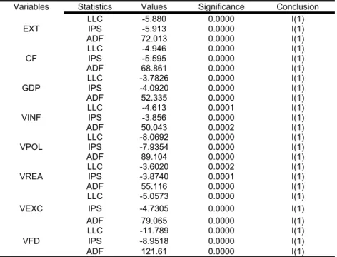
4.1 Results of the panel unit root test
The study applied the three commonly used panel unit root tests. The first is by Levin, Lin and Cho (LLC) (1992), the second Pesaran, Shin and Smith (IPS) (1997), and finally the Fisher-Type Chi- square to examine the non-stationarity properties of the series. These tests are based on the evidence that all the variables are non-stationary under the null hypothesis but accounts for individual heterogeneity among the coefficient. The result is reported in Table 4. From the result, all the variables are integrated of either order one I(1) suggesting that the autocorrection in the dataset is not a problem and can be solved with first differenced and also the Pooled Mean Estimator can estimate the dataset without any difficulties.
Table 4: Result of the panel unit root test
Variables Statistics Values Significance Conclusion EXT
LLC -5.880 0.0000 I(1)
IPS -5.913 0.0000 I(1)
ADF 72.013 0.0000 I(1)
CF LLC -4.946 0.0000 I(1)
IPS -5.595 0.0000 I(1)
ADF 68.861 0.0000 I(1)
GDP
LLC -3.7826 0.0000 I(1)
IPS -4.0920 0.0000 I(1)
ADF 52.335 0.0000 I(1)
VINF
LLC -4.613 0.0001 I(1)
IPS -3.856 0.0000 I(1)
ADF 50.043 0.0002 I(1)
VPOL
LLC -8.0692 0.0000 I(1)
IPS -7.9354 0.0000 I(1)
ADF 89.104 0.0000 I(1)
VREA
LLC -3.6020 0.0002 I(1)
IPS -3.8740 0.0001 I(1)
ADF 55.116 0.0000 I(1)
VEXC
LLC -5.0573 0.0000 I(1)
IPS -4.7305 0.0000 I(1)
ADF 79.065 0.0000 I(1)
VFD
LLC -11.789 0.0000 I(1)
IPS -8.9518 0.0000 I(1)
ADF 121.61 0.0000 I(1)
Source: Computed using E-views 10.0
4.2 Estimation of the Mean-Variance Equation
The presence of the heteroscedasticity in the in the data as shown in Table 3 endorsed the application of the Generalized Autoregression Heteroscedasticity (GARCH) models to estimate the conditional mean-variance equation for each of the macroeconomic variables to avoid the correlation bias as indicated by Kiss and Pontet (2015). The choice of the GARCH (1,1), according to literature is best in capturing the volatility underneath this series and also because it possesses the ability to check the robustness of the model (Kiss and Pontet 2015). According to Enders (1995), in order to ensure that the conditional variance is finite and robust, then it should be such that the coefficient of the GARCH model estimated is close to unity and statistically significant.
From the conditional variance result in Table 5, the estimated innovation coefficients of the GARCH for Cameroon is positive for all the variables and greater than 0.5. This indicates that the
magnitude of the current macroeconomic variables for Cameroon is influenced by their lagged conditional variance. This conditional variance analysis was performed for all the variables for each country in the study. The results were not different from that of Table 5 above, meaning the presence of volatility persists in all the countries analysed. Table 5 presents the GARCH result.
Table 5: Conditional variance of the variables for Cameroon
INF POL REA EXC
Constant 1.2889 85.0737 32399.8 0.2205
Innovation coefficient 0.6338 0.5669 0.9998 0.7405
Standard Deviation 0.0867 0.0000 0.0000 0.0075
Source: Computed using Matlab 14b.
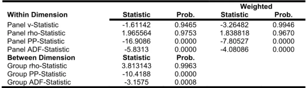
4.3 Results of the panel cointegration test
Before estimating the long run result, the Pedroni (2004) cointegration technique that accounts for heterogeneity by using specific parameters was employed by the paper in analysing the existence of long-run cointegration among the series. This technique employs four-panel statistics (Panel V, Panel rho, panel PP and Panel ADF) and three group statistics (Group rho, Group PP and Group ADF) for which cointegration analysis can be examined. The four-panel statistics are also estimated using the weighted averages making it eleven (11) statistics in all. The panel statistics are computed as the averages of individual autoregressive parameters along the within dimensions of the panel, while the group statistics are based on the pooling the residuals between the dimension of the panel. Table 6 presents the result.
Table 6: Panel cointegration test
Weighted
Within Dimension Statistic Prob. Statistic Prob.
Panel v-Statistic -1.61142 0.9465 -3.26482 0.9946
Panel rho-Statistic 1.965564 0.9753 1.838818 0.9670
Panel PP-Statistic -16.9086 0.0000 -7.80527 0.0000
Panel ADF-Statistic -5.8313 0.0000 -4.08086 0.0000
Between Dimension Statistic Prob.
Group rho-Statistic 3.813143 0.9963
Group PP-Statistic -10.4188 0.0000
Group ADF-Statistic -3.1575 0.0008
Source: Computed using E-views 10
From the estimated result in Table 6, the null hypothesis of no cointegration is rejected at 1% level of significance for six (6) out of the eleven test statistics (11) employed by the Pedroni (2004) cointegration technique. The result proves that the variables chosen for the study are cointegrated such that their short and long-run relationship can be computed using the panel Autoregressive Distributed Lag Model.
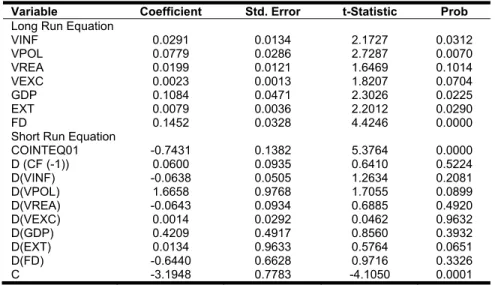
4.4 Results of the panel ARDL
Within the ARDL estimation, the regression estimations are carried out by three (3) separate estimators; the Pooled Mean Group (PMG), the Mean Group (MG) estimation and the Dynamic Fixed Effect (DFE) estimators. This study estimates the ARDL using the Pooled Mean Group (PMG) estimation techniques in the panel ARDL, and the results are presented in Table 7. Due to the heteroscedasticity, associated with the volatility variables, this study takes natural logs of them
to address the underlying heteroscedasticity. The other control variables are in their absolutes values as explained in Table 3.
Table 7: Estimated Long run equation using Pooled Mean Estimation.
Variable Coefficient Std. Error t-Statistic Prob Long Run Equation
VINF 0.0291 0.0134 2.1727 0.0312
VPOL 0.0779 0.0286 2.7287 0.0070
VREA 0.0199 0.0121 1.6469 0.1014
VEXC 0.0023 0.0013 1.8207 0.0704
GDP 0.1084 0.0471 2.3026 0.0225
EXT 0.0079 0.0036 2.2012 0.0290
FD 0.1452 0.0328 4.4246 0.0000
Short Run Equation
COINTEQ01 -0.7431 0.1382 5.3764 0.0000
D (CF (-1)) 0.0600 0.0935 0.6410 0.5224
D(VINF) -0.0638 0.0505 1.2634 0.2081
D(VPOL) 1.6658 0.9768 1.7055 0.0899
D(VREA) -0.0643 0.0934 0.6885 0.4920
D(VEXC) 0.0014 0.0292 0.0462 0.9632
D(GDP) 0.4209 0.4917 0.8560 0.3932
D(EXT) 0.0134 0.9633 0.5764 0.0651
D(FD) -0.6440 0.6628 0.9716 0.3326
C -3.1948 0.7783 -4.1050 0.0001
Source: Computed using E-views 10
A casual observation of the result in Table 7 shows that the long run regression result is more robust as compared with the short run estimates. In the short run, it is only the external debt and political stability volatility that was significant at 10 percent significance level. Therefore, this discussion shall concentrate more on the long run impact of the volatility and other control variables on capital flight. From the results, all the variables are significant except the interest rate volatility, and they all assume the apriori expected positive signs with the only exception being annual GP per capital and financial development which were surprisingly positive even though the apriori expected signs are negative. Macroeconomic uncertainty measured by the inflation rate has a positive impact on capital flight in the SSA as expected and it is statistically significant at 5 per cent level signifying that volatility in the price level in the region plays a significant role in channelling resources from the region. This result is naturally expected as uncertainty around price level will mean a higher cost of investing in the country. Volatility in political stability is also positive and contribute significantly to the exodus of capital in the region. The result shows that a percent increase in fluctuations in political stability releases 7 percent of valuable national resources from the region. In the exchange rate volatility, the result found it to be positive and statistically significant. The theory indicates that distortions in the exchange rate result in the fall of the value of assets invested or profit expected to be generated. This perceived reduction in the asset value or profit may encourage investors rather shift their resources abroad.
Regarding the other control variables, both annual GDP growth and financial development are positive and statistically significant contrary to expectation. Normally, higher economic growth is an indication of higher expected returns on investment and saving. Also, the theory predicts that financial development region also boosts investor confidence in the region and expected to decrease the amount of capital outflow. But the positive impact of external debt on a capital flight is expected as it confirms the revolving door hypothesis in the region. The coefficient and statistically coefficient of the error correction term means that the deviation of the variables from their long-term growth rate is corrected roughly by 74 percent. In other words, the highly significant error correction term suggests that more than 74 % of the instability in the previous year is amended in the current year.
Conclusion and Policy Implications of the Study 5.
This paper investigated the impact of domestic policy uncertainties as perceived by domestic wealth holders on capital flight. The study covers the period between 1990 and 2010 for thirteen HIPC in the SSA region. The variable used to capture the macroeconomic uncertainties included inflation rate volatility, political stability volatility, real interest rate volatility and exchange rate volatility. In addition, other control variables such as external debt, financial development and annual GDP growth were included. The uncertainties of the macroeconomic variables were investigated using the GARCH model. The outcomes of the econometric investigation which reflects the current situation in SSA support the view that domestic investors will withdraw their investments from the country and buy foreign assets if they perceived that the content and direction of current and future public policies are uncertain especially macroeconomics volatility. Volatility in the inflation rate, political stability and exchange rate all undermines the effort to retain valuable capital on the continent. As a recommendation, policymakers in Africa should focus on macroeconomic stability. In that case, there will be stability in the inflation, political institution and exchange rate which will help in reducing the exodus of capital in the region. In addition, the study could not find evidence that improvement in the financial system and growth in the economy can help in reducing the capital flight.
References
Abaidoo, R. (2012). Macroeconomic Volatility and Macroeconomic Indicators among Sub-Saharan African Economies. International Journal of Economics and Finance, 4(10), 1-14.
Agu, C. (2010). Domestic Macroeconomic Policies and Capital Flight from Nigeria: Evidence from a Macro- Econometric Model. Central bank of Nigeria, 48(3), 49.
Ampah, I. K., Gábor, D. K., & Balázs, K. (2018). Capital flight and external debt in Heavily Indebted Poor Countries in Sub-Saharan Africa: An empirical investigation. In Udvari B. – Voszka É. (Eds): Challenges in National and International Economic Policies. University of Szeged, Doctoral School in Economics, Szeged, 135–159.
Atisophon, V., Bueren, J., De Paepe, G., Garroway, C., & Stijns, J. P. (2011). Revisiting MDG cost estimates from a domestic resource mobilisation perspective. OECD Development Centre Working Papers, (306), 1.
Bollerslev, T. (1986). Generalized autoregressive conditional heteroskedasticity. Journal of Econometrics, 31(3), 307-327.
Boyce, J. K., & Ndikumana, L. (2012). Capital flight from Sub-Saharan African Countries: Updated Estimates, 1970-2010. Political Economy Research Institute Research Report (October 2012). University of Massachusetts: Amherst.
Collier, P., Hoeffler, A., & Pattillo. C. (2001). Flight capital as a portfolio choice. World Bank Economic Review, 15(1), 55-80.
Cuddington, J. T. (1986). Capital flight: Estimates, issues, and explanations. Princeton, NJ: International Finance Section, Department of Economics, Princeton University.
Deppler, M., & Williamson, M. (1987). Capital flight: Concepts, measurement and issues. Staff Studies for the World Economic Outlook. Washington, DC: The International Monetary Fund.
Domfeh, K. O. (2015). Capital Flight and Institutional Governance in Sub-Saharan Africa: The Role of Corruption (master’s dissertation, University of Ghana).
Dooley, M. (1986): Country-specific premiums, capital flight and net investment income in selected countries. Unpublished Paper, IMF Research Department, IMF, Washington, DC.
Enders, W. (1995). Applied Economic Time Series. New York: Wiley.
Eggerstedt, H., Hall, R. B., & Van Wijnbergen, S. (1995). Measuring capital flight: a case study of Mexico. World Development, 23(2), 211-232.
Frenkel, J. A., & Goldstein, M. (1991). Exchange rate volatility and misalignment: Evaluating some proposals for reform. In Evolution of the International and Regional Monetary Systems (99-131). Palgrave Macmillan, London.
Fofack, H., & Ndikumana, L. (2014). Capital Flight and Monetary Policy in African Countries. Political Economy Research Institute Working Paper Series, (362).
Hermes, N., & Lensink, R. (2001). Capital flight and the uncertainty of government policies. Economics Letters, 71(3), 377-381.
Im, K. S., Pesaran, M. H., & Shin, Y. (1997). Testing for unit roots in heterogeneous panels. Cambridge Working Papers in Economics, 9526.
Kiss, G. D., & Pontet, J. (2015). The isolation of Sub-Saharan floating currencies. Acta Academica karviniensia, 15(4), 41-53.
Lessard, D. R. & Williamson J. (1987). Capital flight and third world debt. Washington, D.C.: Washington Institute for International Economics.
Levin, A. Lin, C. F. & Chu, C. S. J. (2002). Unit root tests in panel data: asymptotic and finite-sample properties.
Journal of Econometrics, 108, 1, 1–24.
Morgan Guaranty Trust Company (1986). LDC capital flight. World Financial Market, 2, 13–16.
Muchai, D. N., & Muchai, J. (2016). Fiscal policy and capital flight in Kenya. African Development Review, 28(S1), 8-21.
Ndikumana, L. (2016). Causes and effects of capital flight from Africa: lessons from case studies. African Development Review, 28(S1), 2-7.
Ndikumana, L., & Boyce, J. K. (2011). Capital flight from sub‐Saharan Africa: linkages with external borrowing and policy options. International Review of Applied Economics, 25(2), 149-170.
Ndikumana, L., Boyce, J. K., & Ndiaye, A. S. (2014). Capital Flight from Africa: Measurement and Drivers. In Ajayi, S. I. & Ndikumana, L. (Eds.), Capital Flight from Africa: Causes, Effects and Policy Issues. Oxford:
Oxford University Press (Forthcoming).
Nkurunziza, J. D. (2015): Capital flight and poverty reduction in Africa. Capital Flight from Africa: Causes, Effects and Policy Issues, 81-110.
Osei-Assibey, E., Domfeh, K. O., & Danquah, M. (2018). Corruption, institutions and capital flight: evidence from Sub-Saharan Africa. Journal of Economic Studies, 45(1), 59-76.
Pedroni, P. (2004): Panel cointegration: asymptotic and finite sample properties of pooled time series tests with an application to the PPP hypothesis. Econometric theory, 20(3), 597-625.
Polity, I. V. (2016): Political regime characteristics and transitions. Online Database. Retrieved from:
http://www.systemicpeace.org/inscrdata.html.
Ramiandrisoa, O. T., & Rakotomanana, E. J. M. (2016). Why is there capital flight from developing countries?
The case of Madagascar. African Development Review, 28(S1), 22-38.
Salisu, A. A., & Isah, K. (2017). A Capital Flight-Growth Nexus in Sub-Saharan Africa: The Role of Macroeconomic Uncertainty (No. 034). https://ideas.repec.org/p/cui/wpaper/0034.html
Taylor, S. J. (1986): Modelling Financial Time Series. Wiley: Chichester, UK.
UN- Economic Commission for Africa, (2015): Illicit financial flow: report of the high-level panel on illicit financial flows from Africa. http://www.uneca.org/sites/default/files/PublicationFiles/ iff_main_ report_26feb en.pdf.
World Bank (1985): World Development Report. Washington, D. C.
World Bank (2016): World Development Indicators On-line Database. Washington, DC.