Introduction Analysingthetrendovertimeofantibioticconsumptioninthecommunity:atutorialonthedetectionofcommonchange-points

(1)

Analysing the trend over time of antibiotic consumption in the community: a tutorial on the detection of common change-points

Robin Bruyndonckx ^1,2*, Samuel Coenen ^1,3, Niels Adriaenssens^1,3, Ann Versporten¹, Dominique L. Monnet⁴, Herman Goossens¹, Geert Molenberghs^2,5, Klaus Weist⁴and Niel Hens^2,6on behalf of the ESAC-Net study group†

1Laboratory of Medical Microbiology, Vaccine & Infectious Disease Institute (VAXINFECTIO), University of Antwerp, Antwerp, Belgium;

2Interuniversity Institute for Biostatistics and statistical Bioinformatics (I-BIOSTAT), Data Science Institute, Hasselt University, Hasselt, Belgium;³Centre for General Practice, Department of Family Medicine & Population Health (FAMPOP), University of Antwerp, Antwerp, Belgium;⁴Disease Programmes, European Centre for Disease Prevention and Control, Stockholm, Sweden;⁵Interuniversity Institute for

Biostatistics and statistical Bioinformatics (I-BIOSTAT), Catholic University of Leuven, Leuven, Belgium;⁶Centre for Health Economic Research and Modelling Infectious Diseases, Vaccine & Infectious Disease Institute (VAXINFECTIO), University of Antwerp,

Antwerp, Belgium

*Corresponding author. E-mail: robin.bruyndonckx@uhasselt.be

†Members are listed in the Acknowledgements section.

Objectives: This tutorial describes and illustrates statistical methods to detect time trends possibly including abrupt changes (referred to as change-points) in the consumption of antibiotics in the community.

Methods: For the period 1997–2017, data on consumption of antibacterials for systemic use (ATC group J01) in the community, aggregated at the level of the active substance, were collected using the WHO ATC/DDD methodology and expressed in DDD (ATC/DDD index 2019) per 1000 inhabitants per day. Trends over time and presence of common change-points were studied through a set of non-linear mixed models.

Results: After a thorough description of the set of models used to assess the time trend and presence of common change-points herein, the methodology was applied to the consumption of antibacterials for systemic use (ATC J01) in 25 EU/European Economic Area (EEA) countries. The best fit was obtained for a model including two change-points: one in the first quarter of 2004 and one in the last quarter of 2008.

Conclusions: Allowing for the inclusion of common change-points improved model fit. Individual countries investigating changes in their antibiotic consumption pattern can use this tutorial to analyse their country data.

Introduction

The European Surveillance of Antimicrobial Consumption Network (ESAC-Net¹, formerly ESAC) is an international network of surveillance systems that enables data on antibiotic consumption to be collected across the EU/European Economic Area (EEA). With these data, various aspects of antibiotic consumption in the community (i.e. primary care sector), including changing trends in consumption of main antibiotic groups, have been studied in a previous series of articles.^2–7However, while these changes could have occurred gradually, which would require a time-trend, they could also have occurred more abruptly, which would necessitate the inclusion of changes in the time-trend, referred to as change-points.

Comparison of the location of these change-points with the timing of public campaigns could provide valuable insights into the effectiveness of such campaigns.

Change-points, also referred to as transition-points, switch- points or break-points, are usually estimated using either the likelihood framework^8–10or the Bayesian framework.^11–13When comparing the two approaches, the likelihood framework is com- putationally faster and does not require the specification of prior distributions while the Bayesian framework is less sensitive to starting values and allows the location of the change-points to be data-driven.^14,15 For this tutorial, we focus on an adaptive Bayesian model in which both the number of common change- points and their location(s) are data-driven.¹⁶ This model was applied in this series of articles that reviews temporal trends, seasonal variation and presence of change-points, and composition of antibiotic consumption in the community for the period 1997–2017.^17–22

In subsequent sections of this tutorial, the data and the application of the adaptive Bayesian model to antibiotic consumption in

V^C The Author(s) 2021. Published by Oxford University Press on behalf of the British Society for Antimicrobial Chemotherapy.

This is an Open Access article distributed under the terms of the Creative Commons Attribution License (http://creativecommons.org/licenses/

Downloaded from https://academic.oup.com/jac/article/76/Supplement_2/ii79/6328678 by University of Szeged user on 20 October 2021

(2)

the EU/EEA community are presented step by step. The data structure and procedures used to fit the models are presented in Appendix 1 (available asSupplementary dataatJACOnline).

Data

This tutorial explains how a change-point model can be fitted to quarterly data on antibiotic consumption in the community of 25 EU/EEA countries for the period 1997–2017. Data were expressed in DDD (ATC/DDD index 2019) per 1000 inhabitants per day and aggregated at the level of the active substance, in accordance with the WHO ATC classification.²³The methods for collecting the data are described in the introductory article of this series.²⁴The structure of the dataset is presented in Appendix 1 (available as Supplementary dataatJACOnline).

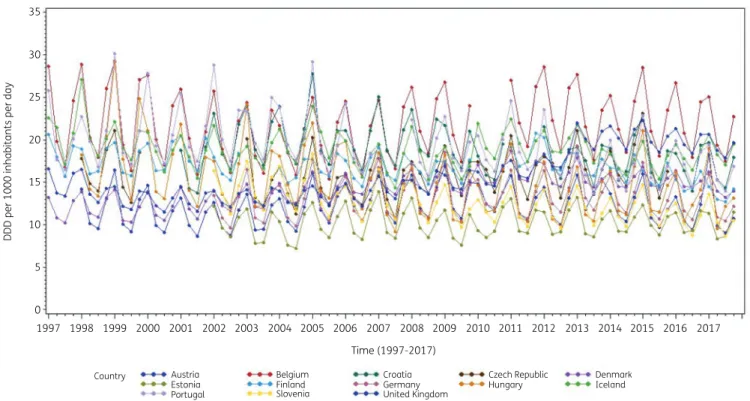
Consumption of antibacterials for systemic use (ATC J01) for a subset of countries that reported quarterly data for at least 15 years during the period 1997–2017 is presented in Figure1.

These longitudinal profiles show clear seasonal variation in antibiotic consumption with upward winter peaks and downward summer troughs, associated with seasonality in viral and bacterial pathogens.²⁵In addition, the profiles demonstrate homogeneity within and heterogeneity across countries. The less complete series were for countries that did not join the network since its start, missed intermittent calls for quarterly data, or did not yet submit quarterly data for the more recent years.

Methodology

The different steps taken in analysing quarterly antibiotic consumption data are described in subsequent sections. An illustration

of how the methodology can be applied is also presented. All models are fitted in a fully Bayesian way. To ensure convergence, we recommend the use of two chains with 110 000 iterations, of which the first 10 000 iterations must be discarded, i.e. burn-in.

Thinning, i.e. discarding samples, to every 5th sample is recommended because of the autocorrelation present for some of the parameters in the model. The code used to fit the models can be found in Appendix 2 (available as Supplementary data at JAC Online).

Model without change-points

To model antibiotic consumption data, we needed a model that accounts for (a) homogeneity in observations within countries, (b) heterogeneity in observations between countries and (c) seasonal variation. One admissible approach is the non-linear mixed model in which random effects represent the country-specific deviations from the average and a sine wave captures the seasonality. An ad- vantage of this model is that it does not require balanced data, which makes it a very suitable approach for modelling the combin- ation of complete and incomplete longitudinal profiles for antibiotic consumption in the community. The non-linear mixed model is formulated as:

Y_ij¼ðb₀þb_0iÞ þðb₁þb_1iÞt_ijþb^S₀þb^S_0iþb^S₁t_ij

sinxt_ijþdþe_ij; (Eq. 1) where Yij is the total antibiotic consumption in the community (in DDD per 1000 inhabitants per day) for countryi(i¼1;2;. . .;N) at timepointtij(j¼1;2;. . .;84), time = 1 corresponds to the start

35

30

25

20

DDD per 1000 inhabitants per day

15

10

5

0

1997 1998 1999

Country Austria Estonia Portugal

Belgium Finland Slovenia

Croatia Germany

Czech Republic Hungary

Denmark Iceland United Kingdom

2000 2001 2002 2003 2004 2005 2006 2007 Time (1997-2017)

2008 2009 2010 2011 2012 2013 2014 2015 2016 2017

Figure 1. Seasonal variation in consumption of antibacterials for systemic use (J01) in the community, expressed in DDD (ATC/DDD index 2019) per 1000 inhabitants per day, in 13 countries reporting consumption per quarter for at least 15 years, 1997–2017.

Bruyndonckxet al.

(3)

of the study (first quarter of 1997),b¼ ðb₀;b₁;b^S₀;b^S₁;x;dÞis a vector of fixed effects whereb₀is the general intercept,b₁is the general change in antibiotic consumption over time,b^S₀is the general amplitude,b^S₁ is the general change in amplitude over time,xis the frequency of the sine wave (¼2p=TwithT¼4) anddis the phase shift of the sine wave,b_i¼ ðb0i;b1i;b^S_0iÞis the vector of random effects whereb0i is the country-specific deviation from the general intercept, b1i is the country-specific deviation from the general change in antibiotic consumption over time andb^S_0iis the country-specific deviation from the general amplitude. We as- sumeb_iNð0;DÞwhereDis a 3%3 diagonal covariance matrix.

We assume that alle_ij are independent and normally distributed with mean zero and constant variancer²_e.

Model with one common change-point

Inclusion of a common change-point, which signals an abrupt change in the evolution of antibiotic consumption over time, modifies Equation 1 as follows:

Yij¼ ðb₀þb0iÞ þ ðb₁þb1iÞtijþ ðb_CPþbCPiÞðtijCPÞ_þ

þðb^S₀þb^S_0iþb^S₁tijÞsinðxtijþdÞ þe_ij; (Eq. 2) where the fixed effects b₀;b₁;b^S₀;b^S₁;x andd, and the random effectsb0i;b1iandb^S_0iare defined as before,xþ=max(x;0), CP represents a common change-point,b_CPis the general difference in the linear trend after versus before the change-point,bCPiis the country- specific deviation from the general difference in the linear trend after versus before the change-point ande_ijis an unexplained error term. The location of this common change-point is data-driven.

Model with additional common change-points

Inclusion of additional common change-points generalizes Equation 2 as follows:

Yij¼ ðb₀þb0iÞ þ ðb₁þb1iÞtijþX^K

k¼1

b_kþ1þbðkþ1Þi

ðtijCPkÞ_þ

þðb^S₀þb^S_0iþb^S₁tijÞsinðxtijþdÞ þe_ij;

(Eq. 3) Wherexþ, the fixed effectsb₀;b₁;b^S₀;b^S₁;xandd, and the random effectsb0i;b1i andb^S_0i are defined as before,Kis the number of common change-points, fork¼1;2;. . .;K,CPkrepresents thek^th common change-point,b_kþ1is the general difference in the linear trend after versus before thek^thchange-point,bðkþ1Þiis the country-specific deviation from the general difference in the linear trend after versus before thek^thchange-point ande_ijis an unexplained error term. The model with one change-point is gradually extended by including additional change-points of which the loca- tions are again data-driven. When including more change-points than present in the data, the model will experience difficulties in obtaining convergence.

Model selection

The Deviance Information Criterion (DIC) is typically used to se- lect the model that explains the data best in a Bayesian

setting.²⁶ The DIC is a Bayesian equivalent to the Akaike Information Criterion (AIC) and is composed as the sum of the posterior expectation of the deviance (D), which measures goodness of fit, and a penalty term for model complexity (pD), which is given by the difference between the posterior expectation of the deviance (D) and the deviance evaluated at the posterior mean (DðhÞ). BecausepD is not invariant to reparame- terization and can become negative, pV [which estimates the effective number of parameters in the model as Var(Deviance)/

2] can be used instead. In model comparison, a smaller DIC represents a better fitting model. Convergence of the algorithm can be checked using trace plots.²⁷

Prior specification

To fit the above models in a fully Bayesian way, prior distributions need to be specified. As a reflection of our lack of knowledge about the regression coefficients, uninformative priors can be used. For the change-points, this translates to a uniform distribution over the whole time-range for the first common change-point, and a uniform distribution over the time-range following the previous change-point for additional change-points to avoid switching of change-points which would result in difficulties with model convergence. For the fixed and random effects, a normal prior with a large variance was used to reflect lack of prior knowledge.

The selected priors are specified as follows:

b₀;b₁;b_ðkþ1Þ;b^S₀;b^S₁;d Normal (0, 1000), independently

withk=1,. . .KandKthe number of change-points,

C1Uniform (1,84), CkUniform (Ck1,84), b0iNormal(0,r²_b

0), b1iNormal(0,r²_b₁), bðkþ1ÞiNormal(0,r²_b

ðkþ1Þ), b^S_0iNormal(0,r²_bS

0). (Eq. 4)

For the hyperparameters, an uninformative inverse gamma distribution is used, which is specified as follows:

r²_b

0;r²_b

1;r²_b

ðkþ1Þ;r²_bS 0

;r²_e IGammað0:001;0:001Þ;independently;

(Eq. 5) wherexIGammaða;bÞmeans that 1=xhas a Gamma distribution with meana=band variancea=b².²⁸

Application of the methodology

We illustrate the methodology discussed above using ESAC-Net quarterly data on antibiotic consumption in the community for 25 EU/EEA countries during the period 1997–2017.

We considered the following models:

Model 1: Non-linear mixed model without change-points Model 2: Non-linear mixed model with one unknown common change-point (C1)

JAC

(4)

Model 3: Non-linear mixed model with two unknown common change-points (C1and C2with C1<C2)

Model 4: Non-linear mixed model with three unknown common change-points (C1, C2and C3with C1<C2<C3)

The results in Table1clearly indicate the need for at least one common change-point, which is reflected by the big decrease in DIC from Model 1 to Model 2. Including an additional unknown common change-point (Model 3) decreased the DIC further.

Including a third common change-point (Model 4) resulted in non- convergence, indicating that a non-linear mixed model with two common change-points (Model 3) was the best fitting model for antibiotic consumption in the community. A summary of the posterior distributions for the model parameters in Models 1–3 is given in Table1.

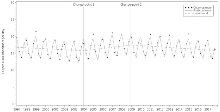
The estimate for the first unknown change-point obtained from fitting Model 2 was 44.529 (last quarter of 2007). Allowing a second change-point, positioned the first change-point at 29.028 (first quarter of 2004) and the second change-point at 48.839 (last quarter of 2008).

The average observed, predicted and predicted linear consumption of antibacterials for systemic use expressed in DDD per 1000 inhabitants per day illustrated that Model 3 fitted the data well (Figure2). The observed and predicted consumption of antibacterials for systemic use expressed in DDD per 1000 inhabitants per day for three selected countries (Belgium, Sweden and the Netherlands) shows that the country-specific predictions closely followed the observed values (Figure3).

Discussion

In this tutorial, the methodology of an adaptive change-point analysis is explained and applied to quarterly data on antibiotic consumption in the community for 25 EU/EEA countries in the period 1997–2017. The inclusion of change-points in the non-linear mixed models used earlier²⁹to describe the trend and seasonal variation in antibiotic consumption over time was motivated by the need to allow for abrupt changes which then could be com- pared with the timing of public awareness campaigns, e.g. the European Antibiotic Awareness Day, policy changes, e.g. changing the reimbursement of antibiotics, or other interventions.³⁰ This analysis can be performed at the third level of the ATC classification, as shown in the example presented here for antibacterials for systemic use (ATC J01), but could also be performed at any other ATC level, e.g. to study the evolution of consumption of amoxicillin/

clavulanic acid over time. Analyses can be performed using consumption data expressed in DDD per 1000 inhabitants per day, as shown in the example presented here, but could also be performed using data expressed in any other metric of antibiotic consumption, e.g. packages or prescriptions per 1000 inhabitants per day. Analyses can be performed for multiple countries, as shown in the example presented here for 25 EU/EEA countries, but could be performed for a smaller subset of countries as well, e.g.

only Northern European countries. Analyses of antibiotic consumption in one specific country could be conducted after removing the now-redundant random effects (boi;b1i;bðkþ1Þi and b^S_0i) from the models. Analyses of yearly antibiotic consumption could be conducted after removing the now-redundant sine wave from the models.

While the fitted change-points were motivated by the need to account for abrupt changes following antimicrobial awareness campaigns, several other events could serve as an explanation for the observed changes in antibiotic consumption. Examples include shortages in specific compounds (e.g. narrow-spectrum penicillins in Belgium),³¹product restrictions (e.g. EMA recommendations on fluoroquinolones),³² changes in package size possibly driven by companies packaging practices,^33,34and accordance of package size with treatment recommendations³⁵ or even a pandemic (COVID-19).³⁶

The models described in this tutorial could be extended by including country-specific latent indicators, thus allowing the common change-point to be switched off for individual countries.

A limitation of this approach is that it hinders convergence, often limiting the model to the inclusion of one common change-point with a country-specific latent indicator. Because the model with two change-points fitted the data best, we did not consider including country-specific latent indicators as a valuable alternative in the current setting. Another option that makes the models described in this tutorial even more flexible would be to include Table 1. Estimates for model fit and parameters: posterior means

(standard errors)

Parameters Model 1 Model 2 Model 3

DIC(pD) 5105.98 4877.68 4759.9

DIC(pV) 5119.56 4958.78 4864.17

b₀ 17.784 (1.258) 17.392 (1.286) 18.046 (1.410) b₁ 0.001 (0.010) 0.014 (0.026) #0.017 (0.022)

b₂ – #0.009 (0.041) 0.054 (0.039)

b₃ – – #0.051 (0.050)

C1 – 44.529 (1.278) 29.028 (1.186)

C2 – – 48.839 (4.168)

b^S₀ 3.790 (0.345) 3.803 (0.351) 3.808 (0.342) b^S₁ #0.012 (0.003) #0.012 (0.002) #0.012 (0.002)

d 0.397 (0.017) 0.397 (0.016) 0.399 (0.015)

r²_b

0 42.970 (14.345) 41.289 (15.914) 40.711 (15.455) r²_b

1 0.002 (0.001) 0.015 (0.007) 0.007 (0.004)

r²_b

2 – 0.035 (0.017) 0.029 (0.014)

r²_b

3 – – 0.042 (0.025)

r²_bS 0

2.543 (0.856) 2.556 (0.847) 2.572 (0.847) r²_e 2.146 (0.084) 1.794 (0.072) 1.646 (0.067)

DIC(pD): Deviance Information Criterion calculated using a penalty term for model complexity (pD); DIC(pV): Deviance Information Criterion calculated using an estimate for the effective number of parameters in the model (pV);b₀, general intercept;b₁, general change in antibiotic consumption over time;b₂, general difference in the linear trend after versus before the first change-point;b₃, general difference in the linear trend after versus before the second change-point;C1, location of the first change-point;C2, location of the second change-point;b₀^S, general amplitude;b₁^S, general change in amplitude over time;d, phase shift of the sine wave;r²_b

0, random intercept variance;r²_b

1, random slope variance;r²_b

2, random difference (after versus before the first change-point) variance; r²_b

3, random difference (after versus before the second change-point) variance; r²_bS

0

, random amplitude change variance; r²_e, residual variance.

Bruyndonckxet al.

(5)

30 Change-point 1 Change-point 2

Observed mean Predicted mean Linear trend 25

20

15

10

5

0

1997 1998 1999 2000 2001 2002 2003 2004 2005 2006 2007 Time (1997-2017)

2008 2009 2010 2011 2012 2013 2014 2015 2016 2017

Figure 2. The average observed (dots), predicted (solid line) and predicted linear (dashed line) consumption of antibacterials for systemic use expressed in DDD (ATC/DDD index 2019) per 1000 inhabitants per day obtained from fitting Model 3.

35 Change-point 1 Change-point 2

30

25

20

15

10

5

0

1997 1998 1999 2000 2001 2002 2003 2004 2005 2006 2007 Time (1997-2017)

2008 2009 2010 2011 2012 2013 2014 2015 2016 2017

Figure 3. The average observed (dots, triangles and stars) and predicted (solid, dashed and dotted lines) consumption of antibacterials for systemic use expressed in DDD (ATC/DDD index 2019) per 1000 inhabitants per day obtained from fitting Model 3 for three selected countries: Belgium, Sweden and the Netherlands from top to bottom.

JAC

(6)

country-specific rather than common change-points (with country-specific latent indicators). However, the added complexity often limits the number of change-points that could be included to one single change-point. Because our main interest was in the trend of antibiotic consumption over time for the EU/EEA, we pre- ferred the inclusion of a higher number of common change-points over the inclusion of country-specific change-points. For individual countries, investigating the trend and changes in their own antibiotic consumption might be a valuable exercise when evaluating the impact of public awareness campaigns, changes in regulations and other national or international interventions.

In conclusion, allowing for the inclusion of common change- points improved model fit. Individual countries investigating changes in their antibiotic consumption patterns can use this tutorial to analyse their country data.

Acknowledgements

We are grateful to the National Focal Points for Antimicrobial Consumption, Operational Contact Points for Epidemiology — Antimicrobial Consumption and Operational Contact Points for TESSy/IT data manager — Antimicrobial Consumption, that constitute the European Surveillance of Antimicrobial Consumption Network (ESAC- Net), for their engagement in collecting, validating and reporting antimicrobial consumption data to ECDC.

Members of the ESAC-Net study group

Reinhild Strauss (Austria), Eline Vandael (Belgium), Stefana Sabtcheva (Bulgaria), Marina Payerl-Pal (Croatia), Isavella Kyriakidou (Cyprus), Jirı´

Vlcek (Czechia), Ute Wolff So¨nksen (Denmark), Elviira Linask (Estonia), Emmi Sarvikivi (Finland), Philippe Cavalie´ (France), Tim Eckmanns (Germany), Flora Kontopidou (Greece), Ma´ria Matuz (Hungary), Gudrun Aspelund (Iceland), Karen Burns (Ireland), Filomena Fortinguerra (Italy), Andis Seilis (Latvia), Rolanda Valint_elien_e (Lithuania), Marcel Bruch (Luxembourg), Peter Zarb (Malta), Stephanie Natsch (the Netherlands), Hege Salvesen Blix (Norway), Anna Olczak-Pienkowska (Poland), Ana Silva (Portugal), Gabriel Adrian Popescu (Romania), Toma´s Tesar (Slovakia), Milan Cizman (Slovenia), Antonio Lo´pez Navas (Spain), Vendela Bergfeldt (Sweden) and Berit Mu¨ller-Pebody (the United Kingdom).

Funding

R.B. is funded as a postdoctoral researcher by the Research Foundation—

Flanders (FWO 12I6319N). N.H. acknowledges support from the University of Antwerp scientific chair in Evidence-Based Vaccinology, financed in 2009#2020 by an unrestricted grant from Pfizer and in 2016–2019 from GSK. Support from the Methusalem finance programme of the Flemish Government is gratefully acknowledged.

Transparency declarations

The authors have none to declare. This article is part of a Supplement.

Supplementary data

Appendixes1and2are available asSupplementary dataatJACOnline.

References

1 European Centre for Disease Prevention and Control (ECDC). European Surveillance of Antimicrobial Consumption Network (ESAC-Net). 2020.

https://www.ecdc.europa.eu/en/about-us/partnerships-and-networks/

disease-and-laboratory-networks/esac-net.

2 Adriaenssens N, Coenen S, Versporten A et al.European Surveillance of Antimicrobial Consumption (ESAC): outpatient antibiotic use in Europe (1997-2009).J Antimicrob Chemother2011;66: vi3–12.

3 Versportern A, Coenen S, Adriaenssens Net al. European Surveillance of Antimicrobial Consumption (ESAC): outpatient penicillin use in Europe (1997-2009).J Antimicrob Chemother2011;66: vi12–24.

4 Versporten A, Coenen S, Adriaenssens Net al.European Surveillance of Antimicrobial Consumption (ESAC): outpatient cephalosporin use in Europe (1997-2009).J Antimicrob Chemother2011;66: vi25–35.

5 Adriaenssens N, Coenen S, Versporten Aet al.European Surveillance of Antimicrobial Consumption (ESAC): outpatient macrolide, lincosamide and streptogramin (MLS) use in Europe (1997-2009.).J Antimicrob Chemother 2011;66: vi37–45.

6 Adriaenssens N, Coenen S, Versporten Aet al.European Surveillance of Antimicrobial Consumption (ESAC): outpatient quinolone use in Europe (1997–2009).J Antimicrob Chemother2011;66: vi47–56.

7 Coenen S, Adriaenssens N, Versporten Aet al.European Surveillance of Antimicrobial Consumption (ESAC): outpatient use of tetracyclines, sulphonamides and trimethoprim, and other antibacterials in Europe (1997-2009).

J Antimicrob Chemother2011;66: vi57–70.

8 Penfold RB, Zhang F. Use of interrupted time series analysis in evaluating health care quality improvements.Acad Pediatr2013;13: S38–44.

9 Lopez Bernal J, Cummins S, Gasparrini A. Interrupted time series regression for the evaluation of public health interventions: a tutorial.Int J Epidemiol 2016;46: 348–55.

10 Hinkley DV. Inference about the change-point in a sequence of random variables.Biometrika1970;57: 1–17.

11 Hall CB, Lipton RB, Sliwinski Met al.A change point model for estimating the onset of cognitive decline in preclinical Alzheimer’s disease.Statist Med 2000;19: 1555–66.

12 Jacqmin-Gadda H, Commenges D, Dartigues J-F. Random changepoint model for joint modeling of cognitive decline and dementia.Biometrics2006;

62: 254–60.

13 Smith AFM. A Bayesian approach to inference about a change-point in a sequence of random variables.Biometrika1975;62: 407–16.

14 van den Hout A, Muniz-Terrera G, Matthews FE. Smooth random change point models.Statist Med2011;30: 599–610.

15 Hall CB, Ying J, Kuo Let al.Bayesian and profile likelihood change point methods for modeling cognitive function over time.Comput Stat Data Anal 2003;42: 91–109.

16 Minalu G, Aerts M, Coenen Set al.Adaptive change-point mixed models applied to data on outpatient tetracycline use in. Stat Model 2013;13:

253–74.

17 Bruyndonckx R, Adriaenssens N, Hens Net al.Consumption of penicillins in the community, European Union/European Economic Area, 1997–2017.

J Antimicrob Chemother2021;76Suppl 2: ii14–ii21.

18 Adriaenssens N, Bruyndonckx R, Versporten Aet al.Consumption of mac- rolides, lincosamides and streptogramins in the community, European Union/European Economic Area, 1997–2017.J Antimicrob Chemother2021;

76Suppl 2: ii30–ii36.

19 Versporten A, Bruyndonckx R, Adriaenssens Net al.Consumption of ceph- alosporins in the community, European Union/European Economic Area, 1997–2017.J Antimicrob Chemother2021;76Suppl 2: ii22–ii29.

Bruyndonckxet al.

(7)

20 Adriaenssens N, Bruyndonckx R, Versporten Aet al. Consumption of quinolones in the community, European Union/European Economic Area, 1997–2017.J Antimicrob Chemother2021;76Suppl 2: ii37–ii44.

21 Versporten A, Bruyndonckx R, Adriaenssens Net al.Consumption of tetracyclines, sulphonamides and trimethoprim, and other antibacterials in the community, European Union/European Economic Area, 1997–2017.

J Antimicrob Chemother2021;76Suppl 2: ii45–ii59.

22 Bruyndonckx R, Adriaenssens N, Versporten Aet al. Consumption of antibiotics in the community, European Union/European Economic Area, 1997–2017: data collection, management and analysis. J Antimicrob Chemother2021;76Suppl 2: ii2–ii6.

23 WHO collaborating centre for drug statistics methodology. ATC Classification index with DDDs 2019. 2018.

24 Bruyndonckx R, Adriaenssens N, Versporten Aet al.Consumption of antibiotics in the community, European Union/European Economic Area, 1997–

2017.J Antimicrob Chemother2021;76Suppl 2: ii7–ii13.

25 Choe YJ, Smit MA, Mermel LA. Seasonality of respiratory viruses and bacterial pathogens.Antimicrob Resist Infect Control2019;8: 125.

26 Spiegelhalter DJ, Best NG, Carlin BPet al.Bayesian measures of model complexity and fit.J Royal Statistical Soc B2002;64: 583–639.

27 Gelman A, Carlin JBB, Stern HSSet al. Bayesian Data Analysis,3rd edn.

Texts in Statistical Science. Chapman and Hall, 2014.

28 Ntzoufras I. Bayesian Modeling Using WinBUGS. John Wiley & Sons, 2009.

29 Minalu G, Aerts M, Coenen Set al.Application of mixed-effects models to study the country-specific outpatient antibiotic use in Europe: a tutorial on longitudinal data analysis.J Antimicrob Chemother2011;66:

vi79–87.

30 Bruyndonckx R, Coenen S, Hens Net al.Antibiotic use and resistance in Belgium: the impact of two decades of multi-faceted campaigning.Acta Clin Belg2021;76: 280–8.

31 Colliers A, Adriaenssens N, Anthierens Set al.Antibiotic prescribing quality in out-of-hours primary care and critical appraisal of disease-specific quality indicators.Antibiotics2019;8: 79.

32 European Medicines Agency (EMA). Quinolone- and fluoroquinolone-containing medicinal products. 2020. https://www.ema.europa.eu/en/medi cines/human/referrals/quinolone-fluoroquinolone-containing-medicinal- products.

33 Frippiat F, Vercheval C, Layios N. Decreased antibiotic consumption in the Belgian community: is it credible?Clin Infect Dis2016;62: 403–4.

34 Bruyndonckx R, Hens N, Aerts Met al.Measuring trends of outpatient antibiotic use in Europe: jointly modelling longitudinal data in defined daily doses and packages.J Antimicrob Chemother2014;69: 1981–6.

35 Rusic D, Bozic J, Bukic Jet al.Evaluation of accordance of antibiotics package size with recommended treatment duration of guidelines for sore throat and urinary tract infections.Antimicrob Resist Infect Control2019;8: 30.

36 Armitage R, Nellums LB. Antibiotic prescribing in general practice during COVID-19.Lancet Infect Dis2021;21: e144.