Detailed study of quantum path interferences inhigh harmonic generation driven by chirped laserpulses

(1)

PAPER • OPEN ACCESS

Detailed study of quantum path interferences in high harmonic generation driven by chirped laser pulses

To cite this article: Tamás Csizmadia et al 2021 New J. Phys. 23 123012

View the article online for updates and enhancements.

Detailed study of quantum path interferences in high harmonic generation driven by chirped laser pulses

Tamás Csizmadia¹^,^∗ , L´enárd Gulyás Oldal¹ , Peng Ye¹ , Szilárd Majorosi¹, Paraskevas Tzallas¹^,² , Giuseppe Sansone¹^,³ , Valer Tosa⁴ , Katalin Varj´u¹^,⁵ , Balázs Major¹^,⁵ and Subhendu Kahaly¹^,⁶^,^∗

1 ELI-ALPS, ELI-HU Non-Proﬁt Ltd., Wolfgang Sandner utca 3., H-6728 Szeged, Hungary

2 Foundation for Research and Technology-Hellas, Institute of Electronic Structure & Laser, GR-70013 Heraklion (Crete), Greece

3 Physikalisches Institut, Albert-Ludwigs-Universität, Stefan Meier Strasse 19, 79104 Freiburg, Germany

4 National Institute for R & D of Isotopic and Molecular Technologies, RO, 400293, Cluj-Napoca, Romania

5 Department of Optics and Quantum Electronics, University of Szeged, D´om t´er 9, Szeged 6720, Hungary

6 Institute of Physics, University of Szeged, D´om t´er 9, Szeged 6720, Hungary

∗ Authors to whom any correspondence should be addressed.

E-mail:tamas.csizmadia@eli-alps.huandsubhendu.kahaly@eli-alps.hu

Keywords:quantum path interference, high-order harmonic generation, dipole phase parameters, Maker fringes, attosecond, ultrashort, atomic and molecular physics

Abstract

We investigate the electron quantum path interference (QPI) effects during high harmonic generation in atomic gas medium driven by ultrashort chirped laser pulses. To achieve that, we identify and vary the different experimentally relevant control parameters of such a driving laser pulse inﬂuencing the high harmonic spectra. Speciﬁcally, the impact of the pulse duration (from the few-cycle to the multi-cycle domain), peak intensity and instantaneous frequency is studied in a self-consistent manner. Simulations involving macroscopic propagation effects are also

considered. The study aims to reveal the microscopic background behind a variety of interference patterns capturing important information both about the fundamental laser ﬁeld and the

generation process itself. The results provide guidance towards experiments with chirp control as a tool to unravel, explain and utilize the rich and complex interplay between QPIs including the tuning of the periodicity of the intensity dependent oscillation of the harmonic signal, and the curvature of spectrally resolved Maker fringes.

1. Introduction

Coherent light sources in the extreme ultraviolet (XUV) and soft x-ray regimes is considered as one of the most useful resources to observe and manipulate various physical, chemical, and biological systems at their natural spatial (nanometric) and temporal (attosecond) scales [1–3]. Due to their relative compactness and low implementation cost, sources based on high harmonic generation in gases (GHHG) [4,5] are the front-runners in generating coherent electromagnetic radiation in the short wavelength domain [6–9].

Being a nonlinear optical process, GHHG can provide a broad spectrum and therefore ultrashort optical pulses in the form of attosecond pulse trains (APT) [10] or even single attosecond pulses [11,12].

Characterization and control of the intensity, temporal spacing, and duration of the individual atto-pulses constituting an APT are of utmost importance in attosecond physics and its applications [13–15]. These properties can be accessed through the investigation and shaping of the XUV spectral (or equivalently temporal) phase behaviour by the simultaneous tuning of speciﬁc parameters of the intense ultrashort laser pulse that drives the high harmonic generation process [16]. In particular, the effect of the fundamental pulse’s chirp on GHHG process has been the subject of studies for several years [17,18], and is still actively pursued [19,20]. The harmonic spectral phase is inherently determined by the microscopic generation process theoretically described by the response of an individual atomic dipole to the strong alternating electric ﬁeld. A simple physical picture of this interaction is provided by the classical model that is built up

(3)

of three distinguishable steps [21]: (1) the emission of a single electron into the continuum (ionization);

(2)accelerationin the continuum over a classical trajectory drawn by the rapidly changing driving electric force and (3)recombination, in which the total (kinetic and potential) energy of the electron is converted into harmonic radiation. Although the classical model gives an intuitive insight into the dynamics of the electron under the inﬂuence of the intense laser ﬁeld and provides good agreement for many experimentally observed features of the harmonic spectrum [22], it does not consider phenomena with quantum

mechanical origin, like phase accumulation due to tunnelling, quantum diffusion of the electron wave packet during propagation, or quantum interference effects. A more realistic semi-classical model was developed by Lewensteinet al[23] incorporating the strong ﬁeld approximation (SFA), where the inﬂuence of the atomic potential during the propagation of the electron wave packet in the continuum is neglected.

The Lewenstein theory obtains the time-dependent dipole moment as D(t)=i

_t

−∞dt _∞

−∞dp E(t)d(p+A(t))d^∗(p+A(t)) exp{iS(p,t,t)}+c.c., (1) In (1) (expressed in atomic units, assuming a negative electron charge),A(t) describes the magnetic vector potential interacting with the target atom;E(t) is the associated electric ﬁeld (E(t)=−∂A(t)/∂t);pis the canonical momentum;d(p)is the dipole matrix element for bound-free transitions; andS(p,t,t) is the quasiclassical action, given by the following expression:

S(p,t,t)= _t

t

dt

[p+A(t)]²

2 +I_p

, (2)

whereIpis the ionization energy. The Fourier transform of (1),D(ωq)=F{D(t)}represents the emitted harmonic spectrum, where the emission rate associated to the harmonic frequencyωq=qω₀ (ω0is the central angular frequency of the driving electric ﬁeld) is proportional toS(ω_q)=ω³_q|D(ω_q)|². The saddle point approximation (or stationary phase approximation, SPA) allows us to convert the continuous integral within (1) to a coherent superposition of quantum paths, which enables the separate investigation of the behaviour and contribution of different electron trajectories within a single emission process [2,24]. Here, the classical electron paths are generalized to complex-valued functions (quantum trajectories), which consist of phase terms equal to the classical actions along the path and suitably assigned amplitudes. When the contributions of various trajectories become comparable, their relative phase difference introduces interference effects (quantum path interference, (QPI)) that play a cardinal role in the formation of the high harmonic spectrum, and can thereby serve as a special tool for probing the atomic dipole and allowing access to the electronic structure and dynamics of atoms or molecules [25–27]. Commonly, high harmonic generation setups can be considered as atomic scale, ultrafast interferometers, where the phase difference between electron trajectories can be altered with the spatial and temporal driving intensityI(r,t), the emitted frequencyω_q, the angle of emissionθ, as well as by various phase matching conditions in the generating medium [28,29]. This physical complexity gives rise to a large variety of experimentally observable interference phenomena.

A simple way to directly perceive QPI is, for example, through the oscillation of the harmonic emission yield either as a result of changing the intensity [30] or the wavelength of the driving electric ﬁeld [31].

Over the past decade, QPI has been extensively studied both in theory and throughout experiments using spectral and spatial filtering techniques [32–34], which has led to powerful applications in attosecond metrology targeting the precisein situmicroscopic level control of the XUV emission process in atoms [35,36] or in aligned molecules [37]. Liuet altheoretically investigated QPI during HHG in argon driven by chirped laser pulses and demonstrated the multi-quantum path interference effect both in a single atom and in macroscopic medium [38]. Recently, detailed interference structures were experimentally observed using chirped, multi-cycle laser pulses: Carlströmet aldiscovered off-axis interference from contributions of long trajectories only, and on-axis interference with the participation of both short and long trajectory groups [39]. Although these studies revealed, both theoretically and experimentally, the dependence of QPI on the chirp of the fundamental laser field, the microscopic details of the underlying electron dynamics influenced by the different chirp-connected features of the driving pulse have not yet been investigated with a comprehensive, self-consistent methodology. Moreover, these researches on QPI driven by chirped pulses so far was conducted on the long pulse (>30 fs) regime, although multiple studies have shown that the trajectory behaviour is significantly altered due to the cycle-to-cycle variation of the fundamental laser pulse [25,40]. This implies that QPI interpretation needs to be handled with care for ultrashort few-cycle pulses, which are now widely available to the community both from table-top laboratory sources, as well as in large-scale facilities like ELI-ALPS.

The purpose of the present paper is to reveal the role of different microscopic mechanisms that result in QPIs during HHG in noble gas atoms exposed to intense, chirped laser pulses. Speciﬁcally, we describe the

(4)

effect of chirp induced, sub-cycle and multi-cycle variations of the driving light pulse on the interference dynamics. The paper is organized as follows: in section2we deﬁne the simple formula of a chirped light pulse with the set of parameter ranges used in our analysis, and depict the details of the model used in the calculations. Sections3–5presents the results obtained through extensive numerical simulations

corresponding to pulses with various peak intensities, durations and instantaneous frequency sweeps. In particular, section3deals with the effect of the pulse duration and high harmonic order on the intensity dependent QPI oscillation utilizing transform-limited pulses as a base scenario. Section4discusses the additional effect of the instantaneous frequency change on the QPI pattern, while section5deals with a realistic chirp model with all aforementioned effects incorporated. Relevant macroscopic calculations are performed in section6. In section7, we discuss the observed alterations of the interference patterns as a function of the applied laser pulse parameters. Finally, section8reports our conclusions.

2. Description of the chirp model

A diversity of chirp models have been utilized in literature [41–46] to emphasize and express different physical aspects through the calculations. An appropriate description of the chirped light ﬁeld that is experimentally accessible and relevant is important for correlating the computational results with

experimental observations. In our case we define the electric field in the spectral domain (E(ω)) so that the spectral intensity (I(ω)∝ |E(ω)|², including both the peak spectral intensity and the bandwidth) is assumed to be unaffected by the chirp, a realistic scenario usually encountered in experiments, where the chirp is introduced by stretching an ultrashort pulse of a fixed energy:

E(ω)=√ 2E0cBπ

Δω exp

−cBπ Δω

2

(ω−ω₀)²

exp(−iφ(ω)), (3)

whereE₀, andΔωare the electric ﬁeld amplitude and the full width at half maximum (FWHM) of the intensity (I(ω)∝ |E(ω)|²) envelope, respectively, andcB=2 ln(2)/π≈0.4413 is the time-bandwidth product for a pulse with a Gaussian envelope.

For ultrashort, chirped light pulses, the spectral phase termφ(ω) in equation (3) is generally presumed to be a smooth function which can be expanded to a Taylor series around theω0central angular frequency as:

φ(ω)=φ0+φ1(ω−ω0)+φ2

2(ω−ω0)²+O(3). (4) This can be approximated with the following formula:

φ(ω)≈ −φCEO−1

2 arctan(ξ)+ξcBπ Δω

2

(ω−ω0)²+O(3). (5) Thereby, for consecutive Taylor coefﬁcients one obtains:

φ0=−ΦCEO−1

2 arctan(ξ), φ1=0, andφ2=2ξc_Bπ Δω

2

, (6)

whereφ₂is the common physical quantity known as group delay dispersion. The Fourier transform of equation (3) (withO(3) phase terms neglected) becomes

E(t)= E0

4

(1+ξ²) exp

− t² τ(ξ)²

cos

ξ t²

τ(ξ)² +ω0t+φCEO

, (7)

whereτ(ξ)=

1+ξ²τ0andτ0= ^√^τ^W,0_c

Bπare the chirped and the transform-limited pulse widths, respectively, andτW,0is the FWHM of the intensity (I(t)∝ |E(t)|²) envelope forξ=0. The calculations were carried out with ﬁelds havingω₀=1.829 rad fs⁻¹central angular frequency (corresponding to a 1030 nm central wavelength) andφ₀=0 carrier envelope offset.E(t) was considered to be linearly

polarized. Equation (7) explicitly shows that three major characteristics—the peak amplitude, the envelope, and the phase—of the transform-limited (ξ=0) driving ﬁeld are altered by the presence of the chirp, all of which have signiﬁcant and distinct impacts on QPI in HHG. In order to benchmark, compare and

differentiate between the effects on the HHG process caused by these distinguishable (but interconnected) chirp induced modifications of the driving pulse, we define three different scenarios, which could also be implemented in real-life experiments. Without any restriction, in general one can rewrite the electric field as:

E(t)= E₀ 4

(1+ξ²_I) exp

− t² (1+ξ_II²)τ₀²

cos

ξIII

t²

(1+ξ_III²)τ₀² +ω0t+φ0

, (8)

(5)

whereξ_I,ξ_IIandξ_IIIare three individual control parameters. It is evident from (8) that the control parameters can be appropriately tuned to probe different aspects of the QPI process:

(I) The peak intensity changes as⁷

I=I0/

1+ξ²_I, (9)

(II) The pulse width is modiﬁed as

τW=

1+ξ_II²τW,0, (10)

(III) The instantaneous frequency within the pulse spans towards higher (ξ_III>0) or lower (ξ_III<0) frequencies within a deﬁned frequency interval that depends on the chirp parameter. The difference between the instantaneous frequencies at the beginning and at the end of the temporal electric ﬁeld can be expressed as:

δωinst=ω(tmax)−ω(tmin)∝ξIII

1+ξ_III² Δω, (11)

whereΔω=cB2π/τ0is the FWHM spectral bandwidth, andtmax−tmin=

1+ξ_III²τ0.

•Ifξ_III=0,ω(t_max)−ω(t_min)=0, the instantaneous frequency does not change in time, there is no chirp.

•If|ξIII| 1,ω(tmax)−ω(tmin)∝ξ_III, the frequency shift linearly varies with the chirp parameter.

•I|ξIII| 1,ω(tmax)−ω(tmin)∝Δω. In this case, the maximum frequency variation covers the bandwidth that matches the known linear nature of chirp (new frequency components do not appear).

Therefore, tuningξ_I(withξ_II=ξ_III=0) in (8) is equivalent to controlling the peak intensity of a transform-limited pulse with a given duration. Variation inξ_II(withξ_I=ξ_III=0) represents a change in transform-limited pulse duration with the same peak intensity, and finallyξ(=ξ_I=ξ_II=ξ_III) indicates the most general case with chirpξ, where the peak intensity and pulse duration are self-consistently modified as mentioned before. In order to investigate the effects of these contributing mechanisms separately, a specific parameter range has been selected (shown in table1) corresponding to the same chirp range

(−3ξ=ξ_I=ξ_II=ξ_III3) in case of all three aforementioned actions. The total applied intensity range in process (I) was chosen considering that it should support the generation of harmonics, while preferably keeping the maximum applied intensity (I₀) relatively low in order to avoid excessive ionization of the medium⁸, thereby preserving the validity of the single-atom simulations. The resulting intensity range deﬁned the chirp parameter regime in table1based on (9). Every computation involved reference atoms having a Gaussian ground state wave function (d(p)=i/(πα_f)^3/4(p/α_f) exp −p²/(2α_f)

), whereαf=I_p is the ﬁtting parameter adjusted to the ionization potential of argon (15.76 eV) [2,23,25]. Recombinations after multiple visits of the parent ion by the accelerating electron have been neglected (therefore only the contributions of trajectories shorter than one optical cycle have been considered). We point out here that the atomic phase shift is neglected in the SFA and it can affect the high-order harmonic spectrum by introducing features that are dependent on the speciﬁc electronic structure of the target atom. The cooper minimum (CM) in argon [47–49] and other ionic [50] or molecular systems [51] is one such

instance. It is worth to note, however, that the location of CM in the high-order harmonic spectrum does not depend on the driving laser intensity and wavelength (see for example ﬁgure 1 in [49,52]) and the spectral phase variation of the harmonics near the CM is observed to be limited to a narrow region near the dip [49,53]. Thus, in general for systems exhibiting CM like behaviour or other intrinsic effects

like giant resonance [54], the experimental conditions can be adapted to either a lower intensity regime, so that the harmonics in the CM region does not reach the plateau of the spectrum, or one can spectrally ﬁlter and select the appropriate harmonic orders to record the QPI patterns, where CM effects do not appear.

7Due to computational reasons, the vector potentialA(t)=−t

−∞E(t)dtwas approximated with the closed-form expression A(t)=−^E0ω0

1

√4

(1+ξ2 ) exp

−_τ(ξ)2^t² sin

ξ_τ(ξ)2^t² +ω0t

for calculating (1). In this case, both the peak intensity (9) and pulse duration (10) slightly depend onξ_III. However, equations (9) and (10) generally provide a very good approximation of the peak intensity and pulse duration, respectively, with a relative error of<5×10⁻³corresponding to the parameter range used in this work.

8Using the set of parameters in table1, the maximum rate of ionization at focus (@ξ=0) would be 3.4%, while @ξ=3 only 0.011% of the atoms would be ionized.

(6)

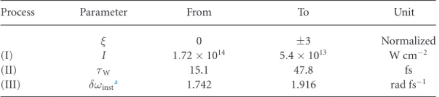
Table 1. The parameter range used in the calculations.

Process Parameter From To Unit

ξ 0 ±3 Normalized

(I) I 1.72×10¹⁴ 5.4×10¹³ W cm⁻²

(II) τW 15.1 47.8 fs

(III) δωinsta 1.742 1.916 rad fs⁻¹

aCalculated atξ_III=3 andt_max−t_min=τ_Wusing (11).

To explain in more details the ﬁner aspects of CM goes beyond the scope of this study. Nevertheless, QPI effects depend strongly on the phase accumulated by the electronic wave packet in the continuum, which is a strong function of the intensity and the temporal shape of the laser ﬁeld in general supporting the validity of the SFA in studying QPI [30,55–57]. Hence, in a differential intensity resolved measurement, such as the one carried out in our work, one would expect that the QPI features would be retained.

Moreover, in order to ensure the validity of the simulations, various single-atom emission spectra calculated with the Lewenstein integral and the saddle point method [2] were compared. We also carried out numerical simulations solving the time-dependent Schrödinger equation with a soft-core Coulomb potential in the single active electron approximation [58] in some cases to justify the correctness of the SFA calculations.

3. QPI driven by transform-limited ultrashort pulses

3.1. Effect of the pulse duration and high harmonic order on the intensity dependent QPI oscillation Following theceteris paribusprinciple, first we investigate only process (I) considering Fourier-limited driving fields (i.e.ξ_II, andξ_III=0 in (8)) with different pulse durations. Alteration in the peak intensity of the driving electric field alters QPI via the modification of the phases of particular trajectories associated to the same harmonic order. The phaseφ^q_j associated to the quantum pathjcontributing to the harmonic orderqis directly connected to the quasiclassical action (equation (2)) and can be approximated by:

φ^q_j ≈ −Upτ_j^q≈ −α^q_jI(in atomic units), whereUpis the ponderomotive energy andα^q_j, known as reciprocal intensity, is roughly proportional to the electron excursion timeτ_j^q[59]. Longer trajectories inherently result in stronger intensity dependence of the corresponding dipole phase. The interference between quantum paths with marginally different excursion times (‘long’ and ‘short’ trajectories) results in an intensity dependent oscillation in the harmonic signal with the angular frequency ofΔα^q=α^q_l −α^qs, correspondingly to their phase difference. This is demonstrated in ﬁgure1(a) for a plateau harmonic (19th) in case of two unchirped pulses with different temporal extents:τW,0=15 fs (blue) and 48 fs (red). Clear oscillations are visible in case of both pulse lengths, although with different oscillation frequencies, Δα^H19(τW,0=15 fs)=4.81±0.12×10⁻¹³cm²W⁻¹for the shorter (blue) pulse, and greater

Δα^H19(τW,0=48 fs)=5.16±0.11×10⁻¹³cm²W⁻¹for the longer (red) pulse. As the harmonic orderq increases,∂φ^q_j/∂Idecreases (increases) for the short (long) trajectories in all half-cycles in the laser ﬁeld, converging towards a common value in the cut-off region [60]. Consequently, differences betweenφ^q_j of differentjtrajectories become smaller, which results in a decrease of the QPI frequency as represented in ﬁgure1(b).

While preserving the oscillation introduced by process (I), we now incorporate the effect of process (II) in order to investigate the dependence of the QPI angular frequency on the transform-limited pulse duration. In this case, the observation in figure1(a) applies in figure1(b) as a general trend, i.e. higher QPI frequencies are produced with the longer driving field in case of all investigated harmonics. This effect is demonstrated in a broader pulse duration range, fromτ_W,0 =12 fs to 48 fs in case of two plateau

harmonics in ﬁgure1(c), where a clear change of the QPI periodicity can be observed for the pulse duration range between approximately 12 and 25 fs, followed by a relatively constant region for pulses longer than 25 fs. In order to gain insight into the underlying processes affecting the QPI frequency as a function of pulse duration and harmonic order, the contribution of different quantum trajectories (havingα^q_j

reciprocal intensities) to the formation of the dipole signal (oscillating with the frequency ofΔα^q) has to be investigated.

3.2. Disentangling quantum path contributions without trajectory analysis

It is possible to disentangle the different quantum path contributions from the dipole moment for several laser peak intensities by using a wavelet-like sliding window Fourier transform on the intensity dependent dipole moment. This simple numerical method has already been utilized by several research groups [61–63]

and it can be viewed as a Gábor-type of analysis on an intensity dependent signal resulting in a 3D

(7)

Figure 1. (a) Oscillation of the single-atom harmonic emission rate as a function of the peak laser intensity in case of two Fourier-limited pulses with different pulse lengths:τW,0=15 fs (blue) andτW,0=48 fs (red). (b) The dependence of the angular frequency of the QPI oscillation on the harmonic order. (c) Variation of the QPI angular frequency with the pulse length using Fourier-limited driving pulses in case of the 19th (green) and 25th (purple marks) harmonic orders. The blue (red) squares in figures1(b) and (c) indicate the same data extracted from the oscillating curve in case of the 15 (48) fs long fields, both depicted in figure1(a).

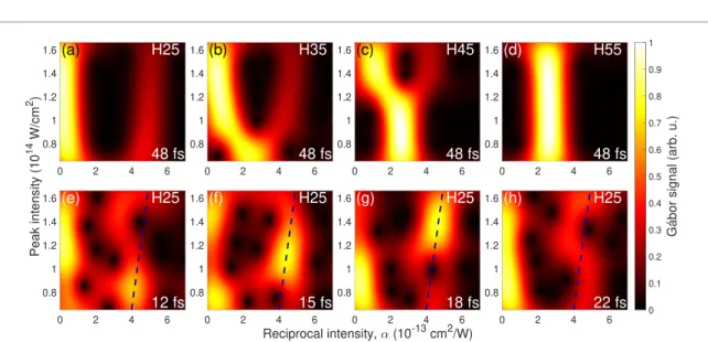
Figure 2. Pseudo-colour maps of the intensity dependent phase behaviour of different harmonic orders (25th (a), 35th (b), 45th (c), and 55th (d)), and in case of pulse lengths (τW,0=12 fs (e), 15 fs (f), 18 fs (g), and 22 fs (h)). AτW,0=48 fs long pulse was used to calculate subplots (a)–(d), while (e)–(h) were evaluated from the dipole phase corresponding to the 25th harmonic.

representation of the intensity (I)—reciprocal intensity (α^q) plane. Speciﬁcally, the Fourier transform is executed on the apodized dipole termd_φ^q(I) consisting of the intensity dependent dipole phase at a given harmonic multiplied by a Gaussian window function:

G(I,α^q)=F{d_φ^q(I)}= _∞

−∞eîφ^q^(I)e^−(a^w^(I^−I))²e^−iα^qÎdI, (12) whereφ^q(I)=arg(D(q,I)), andIis the central intensity for a given apodization window spanning from I1+1/awup to typicallyI2−1/aw, whereI1andI2mark the lowest and highestIintensities of the studied peak intensity range, respectively. The valueawcorresponds to the length of the apodization window and is determined by a trade-off between the resolutions on the intensity and reciprocal intensity axes. In the calculations presented in figure2,aw =5×10⁻¹⁴cm²W⁻¹has been used. By choosing a sufficiently small aw value, (12) practically turns into a Fourier transform resulting in the QPI angular frequency values represented in figure1(b).

Figure2(a) shows that in case of the 25th harmonic, which is located in the plateau region for the entire investigated intensity range, the intensity/reciprocal intensity distribution is dominated by two

distinguishable trajectory classes with marginally differentα^H25_j values, namely short paths (with τs^q<0.6167×2π/ω0andα^H25_s <10⁻¹³cm²W⁻¹) and long paths (withτ_l^q>0.6167×2π/ω0and α^H25_l ≈4–6×10⁻¹³cm²W⁻¹). When the harmonic order is shifted towards higher values (ﬁgures2(b)

(8)

and (c)), theαvalues of the two trajectory groups tend to move towards each other to join as a single class of cut-off trajectory (ﬁgure2(d)) resulting in a smallerΔα^q=α^q_l −α^qs value. Thus this upward shift of the characteristic fork-like structure of the density plots explains the decrease in the QPI angular frequency observed in ﬁgure1(b).

Concerning the pulse length dependence shown in figures1(c) and2(e) reveals that forτW,0 =12.1 fs the contribution of the long trajectory class is strong around one particular intensity (atI≈0.85× 10¹⁴W cm⁻²). At this intensity, theα^H25_l value of the long trajectory (defined as the position of the signal maximum) can be extracted. When tuning the pulse length (figures2(e)–(h)), the maximum is shifted along a linear curve (marked with a dashed dark blue line) until it exits from the studied peak intensity range atτW,0 =22 fs (figure2(h)), while theα^H25_s of the short trajectory remains relatively constant. The Δα^H25values corresponding to different pulse durations are depicted in figure1(c) (with empty dark blue circles and a solid dark blue line as a linear fitting) showing good agreement with the previously calculated QPI angular frequencies.

4. Effect of instantaneous frequency on QPI pattern

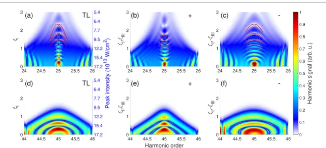
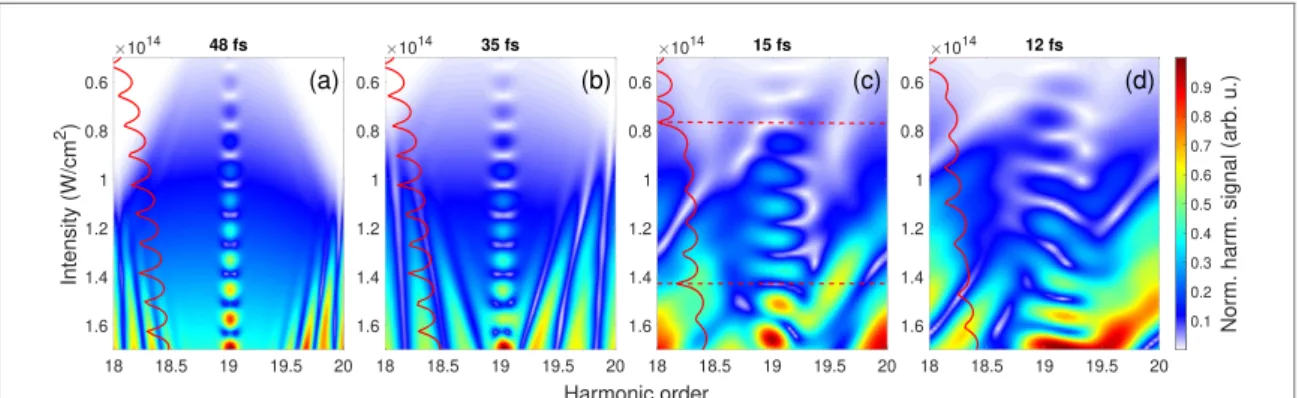
In order to study the effect of the instantaneous frequency variation described in process (III), three intensity-scans (0ξ_I3) were conducted with the use of Fourier-limited (ξ_II=0), positively chirped (0< ξ_III3), and negatively chirped (−3ξ_III<0) fundamental ﬁelds shown in ﬁgures3(a)–(c) and (d)–(e) for spectra around one lower plateau (25th) and one higher plateau harmonic (45th), respectively.

The pulse length of the applied pulses was kept atτW,0=48 fs for all three scans in pursuit of excluding the effect of the pulse length change on the QPI pattern. The fact thatτW,0is fixed (ξ_II=0 or constant) entails that the transform-limited duration is fixed, so the bandwidth is fixed. Figure3shows rich interference patterns in the spectral domain for all three cases. Since the Gábor-type transformation is not able to resolve the intra-pulse dynamics of the driving laser field needed to differentiate between positively and negatively chirped fundamental pulses, we analyse this case by studying the markedly different interference patterns visualized in figure3. Two main effects contribute to the apparent change of the observable textures. The instantaneous frequency of harmonicqcan be described as

ωq(t)=qω0+ ΔωIR,q(t)+ Δωdip(t), (13) whereΔω_IR,q(t) andΔω_dip(t) are the contributions from the instantaneous frequency variation of the driving field and the harmonic chirp caused by the intensity dependence of the atomic dipole phase, respectively [62,64]. At the rising (falling) edge of the pulse, where the intensity increases (decreases), Δω_dip(t) is always positive (negative), which leads to a blue (red) shift at this part of the pulse. These two shifts result in the broadening of the harmonics, provided that no ground state depletion takes place. The broadening is stronger for higher peak intensities (when|∂I/∂t|is greater) at smallerξ_Ivalues, as shown in figure3(a). A positively chirped fundamental pulse contributes with a red frequency shift (Δω_IR,q(t)<0) during the rising edge and a blue shift (ΔωIR,q(t)>0) during the trailing edge that compensates the harmonic chirp resulting in sharp harmonics for highξ_IIIvalues (see aroundξ_III=3 in figure3(b)). On the contrary, a negatively chirped driver further enhances the broadening effect introduced by the intensity dependent dipole phase, resulting in increasingly broadening harmonics with increasingξ_IIIas observed in figure3(c). The frequency chirp of harmonics has been extensively studied both in theory [65–67] and in laboratory experiments [68]. In order to explain the shape of the interference pattern, the instantaneous frequency of harmonicqwas analytically calculated from (13), whereΔωIR,q(t)=2qtξIII/((1+ξ²_III)τ₀²) and Δωdip(t)=α^q_j∂I(t)/∂t. The use of (2) to expressΔωdip(t) results in the following equation:

ΔΩ =ωq(ξI,ξIII)−qω0=±

2qξIII

(1+ξ_III²)τ₀ −α^q_j 4Im

(1+ξ_II²)τ₀

1+ξ_II²

2 ln I0

1+ξ_I²Im

, (14)

whereImmarks certain intensities corresponding to giventntimes, at which the same phase difference between trajectories are sustained for different pulse shapes depending on the applied chirp. In real experimental conditions, theI_mterm refers to intensities at which longitudinal phase matching conditions are optimized spatially and temporally during the simultaneous propagation of the IR and XUV ﬁelds, thereby macroscopic effects are also introduced. Due to the role of phase matching in the formation, these fringes are often referred to as Maker fringes [69–71], even though the shape of the fringe pattern can still be traced back to microscopic mechanisms [70,71]. In our calculations,I_m=I₀/

1+ξ²_I,0, whereξ_I,0 marks the starting points of the curves corresponding toΔΩ(ξ_I,ξ_III)=0. In ﬁgure3, the lines representξ_I andξ_IIIas a function ofΔΩ(assumingξ_II=0 in all cases). Figures3(a), (b) and (c) show lines calculated

(9)

Figure 3. The harmonic spectra around the 25th (a), (b), (c) and 45th (d), (e), (f) harmonics as a function of the chirp parameter in case of (a), (d) transform-limited (ξ_II,III=0,ξ_Ichanges), (b), (e) positively chirped (ξ_II=0,ξ_I,IIIchanges) and (c), (f) negatively chirped (ξ_II=0,ξ_I,IIIoppositely changes) driving pulses. 48 fs long driving pulses were utilized in all six cases.

The same phase difference between short (grey dotted), long (grey dashed), and cut-off (red dot-and-dashed) trajectories were indicated with lines deﬁned by (14) using theα^qvalue of the given trajectory. The red solid lines were calculated with a single intermediateα^qvalue (α^qs< α^q< α^q_l). The square root of the emission rate (

S_q(ω_q)) was plotted (applying also to ﬁgures4 and7) to enhance the visualization of the interference features in the evolving high harmonic spectra.

for the short (grey dotted line), and long trajectories (grey dashed line) at three arbitraryξ_I,0values using theα^H25_j values extracted from the Gábor-type analysis depicted in ﬁgure2. The spectral interference fringes visibly fall between the two lines corresponding to the short and long trajectory groups. The red solid lines were calculated with an intermediate reciprocal intensity value (α^H25_s < α^H25=1.67×10⁻¹³

cm²W⁻¹< α^H25_l ) adjusted for best agreement with the fringe structure. The good overlap between these solid red lines (all nine calculated with the sameα^H25value) and the spectral interference pattern suggests that although the change in the instantaneous frequency of the fundamental beam causes apparent differences between the obtained textures in the vicinity of the 25th harmonic, it leaves theα^q_j reciprocal intensities mainly unaffected. Closer to the cut-off regime of the spectrum, a single reciprocal intensity value (α^H45=2.5×10⁻¹³cm²W⁻¹, extracted from the Gábor-type transformation in ﬁgure2(c)) gives excellent agreement with the fringe pattern, as represented by the red dot-and-dashed lines in

figures3(d)–(f). During the investigation of similar interference features in spectrally and spatially resolved high-order harmonic radiation, Carlströmet alalso found that the curvature of the fringes depends on the mean value (α^q_l+α^qs)/2, as well as on the differenceΔα^q=α^q_l −α^qs, while the fringe periodicity is determined solely byΔα^q. Utilizing this behaviour and a fitting procedure based on an analytical model, it was possible to retrieve the separate dipole phase parameters of the short (α^qs) and long (α^q_l) trajectories from experimentally obtained modulation patterns [39]. It is important to note that the simple analytical model given in equation (14) does not take into account higher order terms in the intensity dependent dipole phase (O(∂²φ^q_j/∂I²)=0), neither does it incorporate the different relative contributions of the trajectories. Such limitation is manifested in figure3(b), where the transition of the interference features from downward concave to downward convex at the harmonic centre is not represented well, despite the correct curvature prediction (with opposite orientation) by equation (14).

5. The combined effect of the fundamental chirp

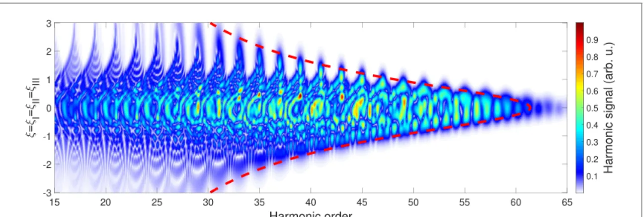
In a real experimental scenario involving the change of the chirp (for example by rotating a plane–parallel plate, translating a wedge-pair or using an acousto-optical modulator), all three of the aforementioned processes must be simultaneously considered (ξ=ξ_I=ξ_II=ξ_IIIin (8)). Figure4reveals complicated interference structures on a spectrogram obtained by a chirp-scan: in case of short generating pulses (corresponding to chirp values from appr.−0.5 to 0.5) the spectral map is dominated by erratic spectral fringes originating from the interferences between the small number of consecutive attosecond bursts.

However, in the multi-cycle regime (|ξ|>0.5), when a well-deﬁned harmonic comb structure is formed, ripples analogous to the previously studied Maker fringes clearly emerge. In addition, features observable at even harmonic orders (in particular at negativeξvalues around−2) are similar to interferences between the long quantum paths only [24]. The combined effect of the harmonic chirp and the instantaneous frequency

(10)

Figure 4. Progression of the single-atom harmonic spectra as a function of chirp parameter (ξ=ξ_I=ξ_II=ξ_III). The dashed red line marks the calculated position of the cut-off. The bandwidth-limited pulse duration wasτW,0=15 fs.

Figure 5. Density plots (F(q,α^q)) obtained by the 2D Fourier analysis (equation (15)) of spectral maps produced with (a) transform-limited (ξII,III=0,|ξ_I|3

15 fs long, (b) transform-limited (ξ_II,III=0,|ξ_I|3) 48 fs long and (c) chirped (0ξ=ξ_I=ξ_II=ξ_III3) generating ﬁelds. The QPI frequencies at which the signal is maximum are marked by dashed white, black and grey lines for case (a), (b) and (c), respectively.|F(q,α)|²is visualized, which was normalized independently for everyqharmonic order to enhance the visibility of the QPI signal.

change of the fundamental ﬁeld results in the ﬁrm sharpening of the harmonic streams for positively chirped generating pulses (ξ >0), and wide, smoothed textures in case of negatively chirped drivers (ξ <0). The cut-off position of each spectrum predicted by the Lewenstein model

(q_cut−off=(F(Ip/Up)Ip+3.17Up)/ω0, whereF(Ip/Up) is equal to 1.32 forIpUpand slowly reaches 1 as I_p/U_pincreases [23]) is marked with the dashed red line in ﬁgure4.

Although the QPI fringes are clearly visible on the spectral map for most plateau harmonics, evaluation of their periodicity is not straightforward due to the constantly varying pulse length, and the overlapping spectral interference patterns. Therefore, a 2D windowed Fourier transform was performed on the spectral maps (S(q,ξ)):

F(q,Δα)= _∞

−∞

_∞

−∞e

(q−q)2 Δq2

S(q,ξ(I))dqe^−iΔαIdI, (15) where a window with the width ofΔq≈1 harmonic order was utilized (figure5). This technique was also used to estimate the error bars—for the points in figures1(b) and (c)—that were defined as the FWHM of the QPI angular frequency signal. The shift between QPI angular frequencies corresponding to different bandwidth-limited pulses—similarly to what was presented in figure1(b)—is clearly noticeable in figures5(a) and (b), when comparing the maxima of the angular frequency signals marked with white and black dashed lines for the transform-limited 15 fs and 48 fs driving pulses, respectively. Figure5(c)

(obtained as the 2D windowed Fourier transform of ﬁgure3) shows a signal located between the white and black dashed lines corresponding to the 15 and 48 fs transform-limited cases, respectively. This is in agreement with the range of pulse durations in the chirped scenario spanning from 15 fs@ξ=0 to 48 fs@ξ=3 according to table1.

(11)

6. Macroscopic effects in QPI

Finally, for a possible experimental observation of the discussed microscopic level interference textures, macroscopic effects (including plasma generation, absorption and refraction during propagation) cannot be neglected. We performed macroscopic simulations using a three-dimensional non-adiabatic model

described in detail in references [72–74].

The applied model consists of three main computational steps. In the ﬁrst step, the propagation of the E(r,t) electric ﬁeld of the fundamental laser pulse (E(r,t)=E(t)f(r), whereE(t)=−∂A(t)/∂t) in the generating medium is calculated by solving the nonlinear wave equation [72]

∇²E(r,t)− 1 c²

∂²E(r,t)

∂t² = ω₀²

c²(1−η_eff²(r,t))E(r,t), (16) wherecis the speed of light in vacuum. The effective refractive indexη_eff(r,t) is calculated as [75]

ηeff(r,t)=η0+ ¯η2I(r,t)−ω²_p(r,t)

2ω₀² , (17)

whereI(r,t)= ¹₂0c|E(r,˜ t)|²is the intensity envelope of the laser ﬁeld (calculated using the complex electric ﬁeldE(r,˜ t) [76]), andω²_p=n_ee²/(m₀) is the square of the plasma frequency (expressed using the number density of electronsne, the elementary chargee, the effective mass of the electronm, and the vacuum permittivity0). Dispersion, absorption, Kerr effect, and plasma dispersion along with absorption losses due to ionization [77] are taken into account via the linear (η₀) and nonlinear (¯η₂) part of the refractive index, respectively. The model assumes cylindrical symmetry (r→r,z) and uses paraxial approximation [75]. By applying a moving frame with the speed of light, and by eliminating the temporal derivative using Fourier transform, the equation to be solved explicitly is

∂²

∂r² +1 r

∂

∂r

E(r,z,ω)−2iω c

∂E(r,z,ω)

∂z =ω²

c²F[(1−η²_eff)E(r,t)]. (18) The solution is obtained using the Crank–Nicolson method in an iterative algorithm [75]. The laser ﬁeld distribution in the input plane of the medium is calculated using the ABCD-Hankel transformation [78].

The second step is the calculation of the single-atom response (dipole momentD(t)) based on the laser-pulse temporal shapes available on the full (r,z) grid, using the Lewenstein integral deﬁned in (1). For the macroscopic nonlinear responseP_nl(t), the depletion of the ground state is taken into account [23,79], giving

P_nl(t)=n_aD(t) exp

− _t

−∞w(t)dt

, (19)

wherew(t) is the ionization rate obtained from tabulated values that were calculated using the hybrid anti-symmetrized coupled channels approach (haCC) [80] showing good agreement with the Ammosov–Delone–Krainov model [81] andnais the number density of atoms in the speciﬁc grid point (r,z) [75,82].

The third and last step is to calculate the propagation of the generated radiationEh(r,t) by the wave equation

∇²Eh(r,t)− 1 c²

∂²Eh(r,t)

∂t² =μ0

d²Pnl(t)

dt² , (20)

withμ₀being the vacuum permeability. Equation (20) is solved similarly to (16), but since the source term is known, there is no need for an iterative scheme. The amplitude decrease and phase shift of the harmonic ﬁeld—caused by absorption and dispersion, respectively—are taken into account at each step when solving equation (20) using textbook expressions describing the effect of complex refractive index on wave

propagation [83]. The real and imaginary parts of the refractive index in the XUV regime are calculated using tabulated values of atomic scattering factors [84].

It was assumed in the calculations that a 15 fs long pulse (in bandwidth-limit) having a Gaussian spatial intensity distribution with 5 mm intensity radius (1/e²) and 187μJtotal pulse energy is focussed into argon gas with a 1 m focal length focussing optics (leading to a 66μmfocussed beam waist) to match the

parameter range used in the single-atom calculations (table1) at the on-axis focal position. The beginning of the generating medium has been inserted at the position of the beam waist (ﬁgure6). The gas medium had uniform pressure distribution of 667 Pa (5 Torr) and 250μmlength along the laser beam propagation axis.

(12)

Figure 6. Schematic illustration of the focussing geometry used for macroscopic simulations. The entry and exit planes are demarcated. The colour map shows the peak intensity of the laser pulse as a function of the spatial coordinates. The blue lines mark the borders of the generation medium, showing that the confocal parameter is much larger than the jet size in this case.

Figure 7. Evolution of the chirp-dependent harmonic spectra around the 25th harmonic during macroscopic propagation in case of (a), (d) transform-limited (ξ_II,III=0,|ξ_I|3) 15 fs long, (b), (e) transform-limited (ξ_II,III=0,|ξ_I|3) 48 fs long and (c), (f) chirped (0ξ=ξ_I=ξ_II=ξ_III3) driving laser ﬁelds. (a)–(c) Response at the beginning of the medium (equivalent to the single-atom response) corresponding to the entry plane of (d)–(f) on-axis macroscopic result at the end of the medium corresponding to the exit plane of this ﬁgure.

Figure7compares the progression of spectral features around the 25th harmonic as a function of the chirp parameter in case of the single-atom response (extracted at the beginning of the generation medium in the on-axis position, figures7(a)–(c)) and after macroscopic propagation (extracted at the end of the generation medium, also in the on-axis point, figures7(d)–(f)) using different, bandwidth-limited or chirped driving pulses. Such near field conditions can be experimentally monitored in multiple manners:

for example the spatial XUV intensity distribution can be mapped onto a spatial ion distribution and recorded with an ion imaging detector (ion microscope) [35,37]. The atomic dipole phase can be directly measured by XUV–XUV interferometry [85,86], or the harmonic radiation can be detected by near field one-to-one imaging (see for example the experimental arrangements in references [9,87]). It is shown in figure7that using the above specified, realistic set of macroscopic parameters results in similar microscopic and macroscopic patterns in case of 15 (a), (d), and 48 fs (b), (e) transform-limited pulses and for chirped (c), (f) pulses as well, even though noticeable alterations naturally happen due to macroscopic propagation.

This similarity can be attributed to the low level of ionization (see the previous footnote II), which induces

(13)

Table 2. Comparison of theΔα^H25values calculated from the modulation of the harmonic signal in case of the single atom, and near ﬁeld macroscopic responses using ﬁgure7and equation (15).

QPI angular frequencies for the 25th harmonic

TL, 15 fs TL, 48 fs Chirped Unit

Single atom 4.47±0.14 4.74±0.12 4.54±0.13 ×10⁻¹³cm²W⁻¹

Macroscopic, near ﬁeld 4.27±0.19 4.48±0.19 4.38±0.15

only slight modiﬁcations of the temporal and spectral features of the composing pulses. The analogy between the microscopic and macroscopic cases is further supported by calculating theΔα^H25angular frequencies of the QPI oscillations in all six instances (table2). Although the oscillation frequency is altered (in this case decreased) by the macroscopic propagation effects, the general tendency of the previous single-atom observations is maintained. The value ofΔα^H25increases with the increasing pulse duration of the transform-limited driving pulses from 15 to 48 fs, while a chirped driving pulse provides an

intermediateΔα^H25value.

The intrinsic intensity dependence of the phases of quantum paths establishes an analogy between spectral and spatial trajectory behaviour for analogous temporal and spatial field envelopes. Therefore, under careful experimental conditions, some of the findings in our paper might be reflected in the far field behaviour of trajectories. For example, the interference pattern in the divergence profiles might get modified, when the pulse duration is changed from the few to the multi-cycle regime due to the interplay between intra-pulse and spatial QPI patterns. To explore such effect, however, a more elaborated

investigation is necessary that takes into account other important macroscopic contributions, such as interferences due to propagation, spatiotemporal coupling [88,89] or special effects entailing advanced pulse forms [90].

7. Discussion

In our present study, QPIs having various microscopic origins have been investigated. In the simplest case, one can consider the superposition of only two (one short, and one long) quantum trajectories within the same optical half-cycle of the laser ﬁeld contributing to the sameqth harmonic of the fundamental laser frequency, causingintra-half-cycleinterference. For a real laser pulse containing multiple optical cycles, this plain picture is expanded by an interplay between trajectories in subsequent half-cycles (intra-pulse interference) that forms spectral QPI patterns. Lastly, the phases of electron trajectories can be tuned pulse-to-pulse by varying the peak intensity of the fundamental laser ﬁeld, leading to another interference-like pattern, which we refer to asintensity dependentQPI pattern. In a macroscopic

environment, this latter QPI pattern is mapped to spatially-resolved interferences stimulated by the spatial intensity distribution of the driving field profile [30,39,70]. Although the complex, chirp (or intensity) dependent harmonic spectrum is formed by the inseparable superposition of these QPI patterns, our results indicate that by varying the driving pulse parameters, the domination of one or the other quantum level phase tuning mechanisms can be observed in the interference structure. This mechanism is illustrated in figure8. When, for example, the generating electric field is temporally long (τW,0 >≈22 fs in our calculations, figures8(a) and (b), the phase difference between long (short) paths in consecutive laser half-cycles is small, which induces constructive intra-pulse interference. This, in turn builds up narrow harmonics around theqth harmonic order. In this case, the intensity-reciprocal intensity density map shows two, clearly separable lines (see figure2(a)) corresponding toα^q_l andα^qs. This results in an intensity

dependent QPI pattern with the observable frequency ofΔα^q=α^q_l −α^qs at harmonic orderq. Contrarily, for very short driving pulses (τW,0 <≈12 fs), the strong modulation of the phases of subsequent long (or short) trajectories through the half-cycle to half-cycle variation of the driving laser intensity creates destructive intra-pulse interference. This is manifested in an erratically behaving spectral QPI pattern, which washes out both the Gábor-type density plot, and the clear beating in the intensity dependent harmonic signal. A very interesting interference happens between these two pulse duration extremes (≈12 fs<τ_W_,0<≈22 fs, ﬁgures8(c) and (d). While well-deﬁned intensity dependent QPI pattern

oscillation is still noticeable in this case, the intra-pulse modulation of the driving field detunes the phases of contributing trajectories in each laser-half-period, especially those of the long trajectories that (due to their longerτ_l^qexcursion times) are more susceptible to the alterations of the electric field. This brings on the modification of theΔα^qoscillation frequency according to figure1(c). The superposition of spectral and intensity dependent QPI patterns is well marked in figure7(a) (calculated with transform-limited 15 fs fundamental pulses), and is also signed by the distortion of the interference pattern (by the occurance of

Detailed study of quantum path interferences inhigh harmonic generation driven by chirped laserpulses

Detailed study of quantum path interferences in high harmonic generation driven by chirped laser pulses

You may also like

Detailed study of quantum path interferences in high harmonic generation driven by chirped laser pulses

considered. The study aims to reveal the microscopic background behind a variety of interference patterns capturing important information both about the fundamental laser ﬁeld and the

1. Introduction

2. Description of the chirp model

3. QPI driven by transform-limited ultrashort pulses

4. Effect of instantaneous frequency on QPI pattern

5. The combined effect of the fundamental chirp

6. Macroscopic effects in QPI

7. Discussion