Local error estimation and step size control in adaptive linear multistep methods

https://doi.org/10.1007/s11075-020-00900-1 ORIGINAL PAPER

Local error estimation and step size control in adaptive linear multistep methods

Carmen Ar ´evalo¹·Gustaf S ¨oderlind¹ ·Yiannis Hadjimichael²·Imre Fekete^2,3

Received: 11 June 2019 / Accepted: 30 January 2020 /

©The Author(s) 2020

Abstract

In ak-step adaptive linear multistep methods the coefficients depend on thek−1 most recent step size ratios. In a similar way, both the actual and the estimated local error will depend on these step ratios. The classical error model has been the asymptotic model,ch^p+1y^(p+1)(t), based on the constant step size analysis, where all past step sizes simultaneously go to zero. This does not reflect actual compu- tations with multistep methods, where the step size control selects the next step, based on error information from previously accepted steps and the recent step size history. In variable step size implementations the error model must therefore be dynamic and include past step ratios, even in the asymptotic regime. In this paper we derive dynamic asymptotic models of the local error and its estimator, and show how to use dynamically compensated step size controllers that keep the asymptotic local error near a prescribed tolerance TOL. The new error models enable the use of controllers with enhanced stability, producing more regular step size sequences.

Numerical examples illustrate the impact of dynamically compensated control, and that the proper choice of error estimator affects efficiency.

Keywords Adaptivity·Time stepping·Step size control·Local error estimation· Linear multistep methods·Dynamic compensator·Variable step size·Differential equations·Initial value problems·Control theory

1 Introduction

We shall consider a standard initial value problem

˙

y=f (t, y), y(0)=y0,

Gustaf S¨oderlind

Gustaf.Soderlind@gmail.com

Extended author information available on the last page of the article.

Published online: 5 June 2020

and letyn denote the numerical approximation toy(tn). Further, we let y_n denote f (tn, yn). Thus derivatives of functions are denoted by a dot, while samples of the vector field are denoted by prime. The methodology developed here does not depend on whether the problem is scalar or a system of equations.

We will study linear multistep methods on nonuniform grids for this initial value problem, of thenormalizedform

yn+1+ k j=1

ak−j,nyn−j+1= k j=0

bk−j,nhny_n−j+1, (1) wherehn = tn+1−tn. Normalization will also be discussed in connection with error constants. The subscriptnof the coefficients indicates that these are rational functions of thestep ratios,ρn−1=hn/ hn−1. The method is implicit ifbk,n=0. We shall consider the grid-independent representation, [1], where every linear multistep method is defined in terms of a fixed set of parameters and interpolation conditions.

Given any grid point distribution{tn}^∞₀ , this representation generates the coefficients ak−j,nandbk−j,n.

Time-step adaptivity is of key importance to make initial value problem solvers efficient. In particular, in stiff problems, where time scales may vary by several orders of magnitude, it is necessary to vary the step size accordingly. If possible, an implementation should offertolerance proportionality, i.e., the global error should be proportional to a preset accuracy requirement,TOL.

The classical approach has been to assume that the local error can be represented asymptotically by

rn=ϕnh^qn, (2)

whereϕnis the norm of the principal error function,hnis the current time step, and rnis the norm of the error estimate. The time step is then typically changed according to the elementary control law

hn+1= TOL

rn

1/q

hn. (3)

For a method of orderp, we takeq=p+1 orq=pdepending on whether the local error per step (EPS) or the local error per unit step (EPUS) is controlled. The scheme is usually accompanied by safety heuristics, and detailed descriptions can e.g. be found in monographs such as [3,6,12,13,17].

Starting in the late 80s, adaptivity based on control theory was developed, [9–

11], leading to [18] and a framework for using digital filters and signal processing, [19,21]. Computational stability was further studied in [20]. Special controllers for explicit and implicit geometric integration were also developed in [14] and [23].

Combinations of these techniques have been applied to near-Hamiltonian problems with weak Rayleigh damping, [16].

This theory has focused on one-step methods, for which the asymptotic error model (2) applies whenever the tolerance is small enough. Taking logarithms, (2) becomes

logrn=q·loghn+logϕn, (4)

suggesting that a step size change affects the error (approximately) by a constant

“gain” factor ofq, without any dependence on step size history. While this static error model is correct for one-step methods in the asymptotic regime, it is no longer correct outside asymptotic operation, [10].

For a k-step linear multistep method it is not even correct in the asymptotic regime. As the method coefficients depend on k−1 past step ratios, errors are similarly affected, and the error’s step size dependence becomes dynamic. Never- theless, the elementary controller (3) has been applied to multistep methods, with varying success. Unfortunately, its stability may deteriorate in combination with e.g.

the Adams–Bashforth methods. Thus, depending on the choice of error estimator, the dynamic interaction of method and controller may become resonant and oscillatory.

The problems can be overcome by a careful combination of method, estimator and controller.

In order to improve adaptive multistep methods, we shall investigate newdynamic error modelsofmultiplicative form,

rn =ϕnh^qn· s j=1

ρ_n^δj_−j. (5)

Here the first factor is identical to the static model (2). The second factor accounts for step size history in terms of step ratiosρn−j = hn−j+1/ hn−j. The number of past step ratios iss=k−1 for ak-step method ifrnrepresents the actual error, while it iss =kfor error estimators that use additional data from one previous step. The parametersδjare characteristic of each multistep method and its error estimator.

In multistep methods, there is a concern over zero stability when the step size varies, focusing on how large step ratios can be allowed without causing instabil- ity, see e.g. [5,7,8,22]. While this issue is of significance, it does not reflect that feedback control interacts with the method and manages overall stability. Thus, in a strongly zero stable method a stable computational process can be maintained by generating a smooth step size sequence (i.e., having step ratiosρn ≈1). This can be achieved by a well designed controller, working with incremental step size changes, avoiding traditional step size halving/doubling.

The grid-independent approach to multistep methods has also been implemented in a proof-of-concept software platform, [2], where any multistep method can be evaluated underceteris paribusconditions. While the theory makes it possible to find method-specific dynamic error estimators in terms of current and past step sizes, the implementation has so far only offered controllers for the static model (2). Our main objectives in this paper are therefore1)to analyze dynamic error estimators, based on models of the form (5); and2)to devise suitable controllersthat manage the local error as well as the stability of the interaction of method and controller. Our approach is based on using discrete control theory as outlined in [19].

The main result is that we construct a dynamic compensator that extracts the static part of the asymptotic error model from the estimator, allowing us to employ standard digital filters and other controllers to achieve results comparable to those of one- step methods. We further show that without this dynamic compensation, conventional techniques are not completely reliable. Thus, for example, the elementary controller

(3) is unsuitable for the control of adaptive linear multistep methods, as the stability margin of the process deteriorates with increasing step size history dependence.

2 Dynamic error models and control objectives

In the classical constant step size theory, the local error of a multistep method has an asymptotic expansion with leading term

ln=c^∗h^p+1y^(p+1)(tn), (6) ash → 0, wherec^∗ is referred to as the method’s (normalized)error constant. But this assumes that all steps shrink simultaneously. In adaptive methods, however, hav- ing reached the pointtn+1=tn+hn, we consider changing the next step size,hn+1, but none of the previously accepted stepshn, . . . , hn−k+1. As a consequence, the asymptotic error will depend on previous step ratios.

Local error control is justified by the possibility of linking a local error bound to the global error via tolerance proportionality. Global error accumulation can be modeled by the variational equation,u˙=J (t)u+w, whereJ (t)=∂f/∂yalong the exact solutiony(t). Hereu(t)andw(t)represent global and local errors, respectively.

Letμ[J (t)]denote the logarithmic norm ofJ (t), and assume thatμ[J (t)] ≤Mfor allt ≥ 0. Note thatMmay be negative. Further, letw∞=maxt≥0w. Then a global error bound can be obtained by integrating the differential inequality

d

dtu ≤M· u + w∞

over a single step to obtain

u(t+h) ≤e^hMu(t) +e^hM−1

M w∞. (7)

Innonstiff computation, we have|hM| 1. Apart from the error propagation, the global error is then incremented by approximatelyhw∞in a step of lengthh. By using the control objectivew∞ ≤ ^TOLwe keep the global error growth rate in check and achieve tolerance proportionality. This corresponds to local error per unit step (EPUS) control.

If on the other hand−hM 1, modelingstiff computationand strong damping, the exponential terms in (7) can be neglected, and we have

u(t+h)−w∞

M = −hw∞

hM hw∞.

Thus, with little or no error propagation, the global error effectively equals (a fraction of) the local error. To achieve tolerance proportionality, it is then sufficient to use the control objectivehw∞≤^TOL, corresponding to local error per step (EPS) control.

The choice ofEPUSorEPSdetermines the powerqin the error model, but by suitably expressing the controller’s parameters in terms ofq, one can obtain similar overall dynamics for both control objectives as well as for methods of different orders.

Inserting the exact solutiony(t)into (1), we obtain a residual, y(tn+1)+

k j=1

ak−j,ny(tn−j+1)− k j=0

bk−j,nhny(t˙ n−j+1)= −˜ln, (8) wherel˜n = c(ρ¯n) h^pn⁺¹y^(p+1)(tn). Compared to (6), the error constantc^∗has been replaced by a functionc(ρ¯n), which depends on thek−1 most recent step ratios, collected in the vectorρ¯n=(ρn−1, . . . , ρn−k+1). Lettingun=yn−y(tn)denote the global error, we subtract (8) from (1) and linearize to obtain

un+1+ k j=1

ak−j,nun−j+1− k j=0

bk−j,nhn[J (tn−j+1)un−j+1+ l˜n

b(ρ¯n)hn] =0, whereb(ρ¯n) = k

0bk−j,n. This is the multistep discretization of the variational equationu˙=J (t)·u+w. The functionwis constant within each step, and

w= l˜n

b(ρ¯n)hn =y^(p+1)(tn) h^pn·π(ρ¯n), (9) whereπ(ρ¯n)=c(ρ¯n)/b(ρ¯n)introduces dynamics into the error model.

In constant step size theory,ρ¯ =(1,1, . . . ,1)=1. The method is often normal- ized so thatb(1)=1, implying thatc(1)=c^∗, cf. [12, p. 373]. It then follows that π(1)=c^∗. Since we have used the normalizationak,n=1 instead, the error constant is affected. Letπ (ˆ ρ)¯ =π(ρ)/π(1). Then (9) becomes¯

w= ˆc^∗y^(p+1)(tn) h^pn · ˆπ (ρ¯n), (10) making the error constantcˆ^∗=π(1)conform to the method normalization and error propagation model above. For the Adams methods, it always holds thatb(ρ¯n)≡1, implying thatcˆ^∗=c^∗even when our normalization is used.

For general multistep methods, we have thus arrived at the error model

rn=ϕnh^qn· ˆπ (ρ¯n), (11) withq =pforEPUScontrol andq=p+1 forEPS. Letδ¯= {δj}^s1be given by the gradient

δ¯^T=grad_ρ¯π (ˆ ρ)¯ _¯

ρ=1. (12)

Assume thatρ¯n=1+ ¯vnwith¯vn∞1. It follows that logρ¯n ≈ ¯vn, and logπ (ˆ ρ¯n)≈log

1+ ¯δ^T· ¯vn ≈ s j=1

δjvn−j ≈ s j=1

logρ_n^δj_−j =log s j=1

ρ_n^δj_−j. Hence the approximationπ (ˆ ρ¯n)≈s

1ρ_n^δj_−j is accurate to O(¯v²_∞), and establishes the multiplicative dynamic error model (5). This approximation enables the design of a controller that compensates the specific linear dynamics of the error. It is also a necessary simplification when the step numberkis large, as the rational function

ˆ

π (ρ¯n)consists of multinomials with a very large number of terms. For this reason, the determination of the powersδj typically requires symbolic computation.

The error model is best illustrated by studying a simple example, and we choose the two-step Adams–Bashforth (AB2) of order p = 2. In the grid-independent formulation [1] the adaptive AB2 method reads

yn+1=yn+

1+ρn−1

2

hny_n −ρn−1

2 hny_n−1, (13) wherehn = tn+1−tn. The local errorrn = y(tn+1)−yn+1 at tn+1 is found by inserting exact data, i.e.,yn=y(tn),y_n = ˙y(tn)andy_n−1= ˙y(tn−1), and expanding in a Taylor series to obtain the asymptotic error expression

l˜n≈ 5 12

...y (t_n+1)h³_n 2

5+ 3

5ρn−1

, (14)

where higher order terms (here fourth order in the step size) have been neglected. For constant step size (ρn−1 =1) we recognize the classical asymptoticprincipal error functionof the AB2 with its error constant, asϕn=5...

y /12.

For variable steps, we now have ˆ

π (ρ)= 2 5+ 3

5ρ ⇒ δ1= ˆπ(1)= −3

5. (15)

Consequently, the asymptotic local error model in multiplicative form (5) is

l˜n≈ϕnh³_n·ρ_n⁻₋^3/5₁ =ϕnh^12/5n h^3/5_n−1. (16) While “dimensionless,” the step ratio does not affect the orderq, but modifies indi- vidual powers of the step sizes. This has little influence onerror magnitude (as ρn−1≈1) but altersstep size dynamicsand the subsequent control design.

In one-step methods, the elementary controller is derived from (2) by assuming thatϕ is slowly varying along the solution to the differential equation. Thus, if the errorrndeviates fromTOL, the next step size can be chosen to makern+1≈^TOLby solving

TOL=ϕn+1h^q_n+1, (17)

forhn+1, assuming thatϕn+1 =ϕn. Dividing (17) by (2) we obtain the control law (3), known as adeadbeat controller, [19]. This has finite impulse response (FIR), since an impulse in the sequence{ϕj}^∞0 will be compensated by the controller in a finite number of steps, in this case a single step. In fact, it is easily shown that the control law yieldsϕnh^q_n+1 ≈^TOL, i.e., the proposed step size is matched to the previous value of the principal error function.

The same intuitive approach could be considered for multistep methods. Assuming thatϕn+1=ϕnin the AB2 method and dividing the two equations

TOL = ϕn+1h^12/5_n+1h^3/5n

rn = ϕnh^12/5n h^3/5_n−1 results in the control law

hn+1= TOL

rn

5/12

ρ_n⁻₋^1/4₁ ·hn. (18)

Apart from the unexpected power ofTOL/rnin (18), the controller has an extra factor due to the error’s dynamic character. Perhaps more surprisingly, (18) is not deadbeat, and has a less desirable behavior.

There are also alternative ways to estimate the error, and a few will be described in detail in Section5. Above, the error (16) was obtained by Taylor series expansion. It can be computed in practice, using a comparison method (at least) one order higher than AB2, say the AB3, operating in the asymptotic regime. Another common esti- mation technique is to compare the results from two methods of the same order. This is similar to the classical predictor–corrector technique. Thus, if the AB2 method is represented as a method constructing a polynomial of degree 2, the error can be esti- mated by comparing this polynomial attn+1to the result obtained by extrapolating the corresponding polynomial, constructed on the previous step. While crude, this difference can still be used to compute an asymptotically correct error. The dynamic asymptotic error model is then more complex,

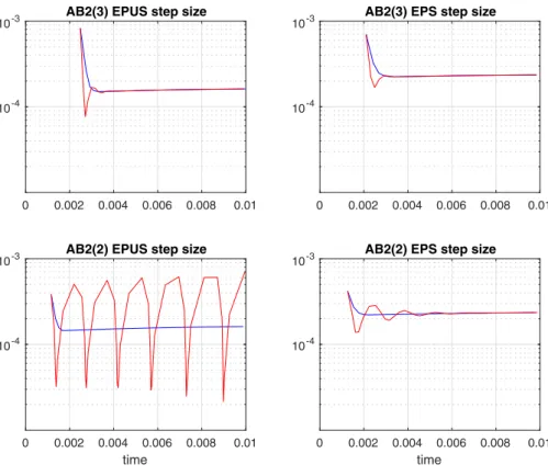
rn=ϕnh^qnρ_n⁻₋^45/23₁ ρ_n⁻₋^12/23₂ . (19) An attempt to derive control laws by the simple approach used above fails, and results in unstable controllers, both inEPUSandEPSmodes. The elementary control law (3) fares a little better, and is stable inEPSmode in combination with (19), but unstable inEPUSmode. Thus, if methods, estimators and controllers are combined arbitrarily, performance is often underwhelming, see Fig.1, where the elementary controller is compared to one of the dedicated dynamically compensated controllers we will develop in this paper. This motivates a thorough investigation of error estimation and step size control for adaptive multistep methods, focusing on the dynamics of the error model.

3 Tools from linear control theory

In the implementation of a discrete time system, it is important to synchronize vari- able indexation. When using theztransform, all variables, sequences and transforms are expressed in relation to the reference indexn, corresponding to the pointtn, and we use the following time domain numbering convention:

1. Given the numerical solution(tn, yn), the method takes a step sizehnto compute yn+1attn+1=tn+hn

2. The method produces an error estimatern attn+1, modeled in the asymptotic regime by an error model such as (5)

3. The controller computes the next step size ratioρnfromrn

4. The controller then updates the step size according tohn+1=ρnhn

5. The computational process repeats from 1.

We shall analyze this process using linear control theory, which is based on the analysis of linear difference equations. The multiplicative forms of the error model and controller are necessary, since they can be converted to difference equations by taking logarithms, after which theztransform is used to analyze stability and

0 0.002 0.004 0.006 0.008 0.01 10^-4

10^-3 AB2(3) EPUS step size

0 0.002 0.004 0.006 0.008 0.01 time

10^-4 10^-3

AB2(2) EPUS step size

0 0.002 0.004 0.006 0.008 0.01 10^-4

10^-3 AB2(3) EPS step size

0 0.002 0.004 0.006 0.008 0.01 time

10^-4 10^-3

AB2(2) EPS step size

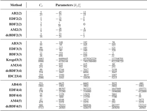
Fig. 1 The AB2 method is combined with two different error estimators and two different controllers, running inEPUSandEPSmodes. Top panels show emulated step size sequences with a pre-constructed ϕ(t)for AB2(3) with third order error estimator. Lower panels show corresponding data for AB2(2) with second order error estimator. The tolerances wereTOL=2·10⁻⁶(EPUS) andTOL=10⁻⁹(EPS), respec- tively. Oscillatory sequences (red) are due to resonances, caused by the elementary controller (3). Smooth sequences (blue) are generated by a dynamically compensated controller with vastly improved stability.

Lower left panel shows that AB2(2) is unstable inEPUSmode when the elementary controller is used (red)

frequency response. For a simple demonstration of this procedure, let us consider (5) fors=2, i.e.,

rn=ϕnh^qn·ρ^δ_n¹₋₁ρ_n^δ2₋₂=ϕnh^qn^+δ1h^δ_n²₋⁻₁^δ1h⁻_n−^δ2₂. (20) Now, taking logarithms in (20), we obtain the difference equation

logrn=G(E)loghn+logϕn, (21) whereEis theforward shift operator, informally defined byEun = un+1for any discrete sequence. The rational functionGis defined by

G(z)=q+δ1+(δ2−δ1)z⁻¹−δ2z⁻²= (q+δ1)z²+(δ2−δ1)z−δ2

z² . (22)

Note that, due to the structure of (20), it follows thatG(1)=q.

We leth = {hj}^∞0 denote the entire sequence of step sizes, and use the simpli- fied notation logh = {loghj}^∞0 . A standard tool in discrete control theory is thez transform, defined for the sequence loghby

(Z logh)(z)=^∞

j=0

(loghj)z^−j.

Since the risk of misunderstanding is minimal, with a slight abuse of notation we follow [19] and let loghdenote theztransform of the sequence logh. Theztransform of the linear difference equation (21) is then

logr=G(z)logh+logϕ. (23)

The functionG(z), referred to as theprocess model, is theztransform of the operator associated with thestep size–error relation(21), while the additive term logϕ is an external disturbancecorresponding to the principal error function, which is to be

“rejected” by the controller. This means that the controller adjusts the step size to counteract the influence of logϕ.

In order to control the error magnitude by adjusting the step size, the error sequence logris compared to the tolerance logTOL, and the sequence

log^TOL

rj

_∞

0

=logTOL−logr

is referred to as thecontrol error. The controller aims to eliminate the control error, continually adjusting the step size according to thecontrol law

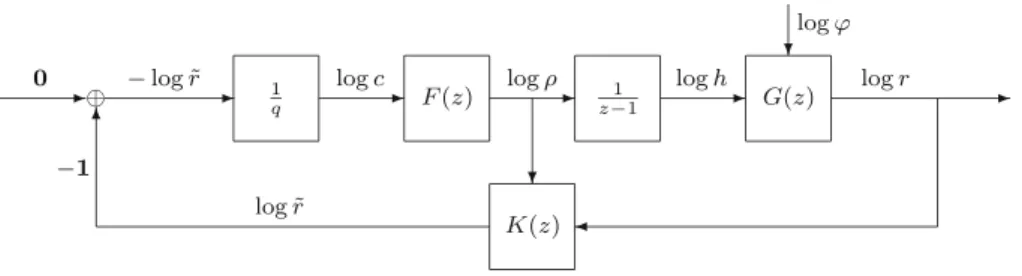
logh=C(z)·(logTOL−logr), (24) where C(z) is the z transform of the linear difference operator associated with the controller. The overall interaction between process and controller is usually represented by a block diagram, see Fig.2.

Next we analyze the process–controller interaction. Combining the control law with the process model, we have the linear system

logh+C(z)logr = C(z)logTOL

−G(z)logh+logr = logϕ.

Fig. 2 Time step adaptivity viewed as a feedback control system. Represented by the transfer function G(z), the computational process takes loghas input, producing an error estimate logr =G(z)logh+ logϕ. The principal error function logϕenters as an additive disturbance, to be compensated by the con- troller. The error estimate logris fed back and compared to logTOL. The controller, represented by its transfer functionC(z), constructs the next step size through logh=C(z)·(log^TOL−logr). All sequences, as well as the controller and the process, are represented by theirztransforms

Solving for loghand logrin terms of the data logϕand logTOL, we obtain logh = Hϕ(z)logϕ+HTOL(z)logTOL

logr = Rϕ(z)logϕ+RTOL(z)logTOL,

where we identify the fourclosed loop transfer functions, from logϕ and logTOL

respectively, to loghand logr. As the constantTOLis of little interest, we takeTOL= 1 (logTOL := 0), meaning that the error is measured in units of TOL. Note that changing the constantTOLhas no effect on the error, sinceRTOL(z)logTOL=0 for any constantTOL. Likewise, it has little effect on the step size, other than adding a constant to the step size sequence logh.

Thestep size transfer functionanderror transfer functionare, respectively, Hϕ(z) = − C(z)

1+C(z)G(z); Rϕ(z) = 1

1+C(z)G(z). (25) The asymptotic process model G(z) is found by analyzing the error estimator of a given linear multistep method, while the controllerC(z) can be chosen to meet various design criteria for stability and smooth step size sequences.

The closed loop transfer functions have the same poles, which correspond to the zeros of the characteristic equation and govern stability. They must remain well located inside the unit circle. It is sometimes possible to constructC(z)so as to move all poles toz=0, corresponding todeadbeat control.

To model a bounded, quasi-periodic input one frequency at a time, we take logϕ = {e^iωn}forω∈ [0, π], withω =π corresponding to the highest discrete frequency, logϕn=(−1)ⁿ. For such periodic inputs, it holds that

logh=Hϕ(e^iω)logϕ; logr=Rϕ(e^iω)logϕ

where the complex valueHϕ(e^iω)reveals the phase and amplitude of the step size sequence compared to the input logϕ = {e^iωn}. Disregarding phase, thescaled step size frequency responseand theerror frequency responseare given by, respectively,

Ah(ω)= |qHϕ(e^iω)| ; Ar(ω)= |Rϕ(e^iω)|, (26) where the extra factor ofq in |qHϕ(e^iω)| normalizes the step size attenuation so thatAh(0) =1. This factor is only a matter of convenience, reflecting that for the asymptotic process it always holds thatG(1)=q.

Step size and error attenuations are dimensionless ratios, measured in theISOunit of decibel (dB), defined by 20·log₁₀Ah(ω). Thus an attenuation of+20 dB corre- sponds to an amplification by one order of magnitude. Likewise, an attenuation of

−6 dB corresponds to a damping by a factor of 2.

The zeros (if any) of the step size transfer function|qHϕ(z)|block signal trans- mission. Thus, selectingC(z)such thatAh(π )=0, one can design low-pass digital filters that suppress noise and produce smooth step size sequences. This is covered in detail for the static processG(z)=qin [19,21].

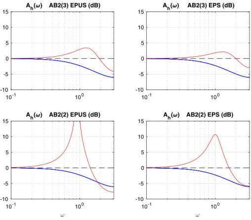
In Fig. 3we plot the step size frequency responses corresponding to the AB2 method operating inEPUSandEPSmodes, using two different error estimators and the same two controllers as in Fig.1, with a one-to-one correspondence between the plots. As before, the designation AB2(3) refers to a third order error estimator,

10^-1 10⁰ -10

-5 0 5 10 15

A_h( ) AB2(3) EPUS (dB)

10^-1 10⁰

-10 -5 0 5 10 15

A_h( ) AB2(3) EPS (dB)

10^-1 10⁰

-10 -5 0 5 10 15

A_h( ) AB2(2) EPUS (dB)

10^-1 10⁰

-10 -5 0 5 10 15

A_h( ) AB2(2) EPS (dB)

Fig. 3 Frequency response diagrams show step size attenuation when the AB2 method is combined with two different controllers, and two different error estimators inEPUSmode (left panels) andEPSmode (right panels). The elementary controller (red) has strong resonances nearω≈ 1, making it unsuitable for multistep methods. With the third order estimator (top panels) the resonance is less pronounced. By contrast, a dynamically compensated controller (blue) eliminates the resonance and offers additional high frequency suppression, generating smooth step size sequences. Dashed black reference curve represents deadbeat control. Attenuation is measured in decibels, dB

while AB2(2) refers to a second order estimator. For the latter, the frequency response reveals that the elementary controller has a damaging resonance nearω ≈ 1. This contaminates the transient performance of the elementary controller, even causing the unstable oscillatory behavior inEPUSmode observed in Fig.1. AlthoughEPUS

mode is always worse thanEPS, the resonance is much less prominent for the third order estimator. There are two conclusions to be drawn. First, as performance differs strongly, it is important to combine good error estimators with controllers so as to avoid resonance and instability. While the choice of error estimator is important, a dynamically compensated controller is always better than the elementary controller, which isunsuitable for multistep methods. Figure3demonstrates that a dynamically compensated controller cannot only manage the benign third order estimator, but also the second order estimator, with a nearly uniform behavior, irrespective of whether the objective isEPSorEPUS.

4 Control analysis of dynamic error models

Beginning with two-step methods, we assume that a computable error estimator can be modeled nearρ¯=1by

rn=ϕnh^qn·ρ^δ_n¹₋₁ρ_n^δ2₋₂=ϕnh^qn^+δ1h^δ_n²₋⁻₁^δ1h⁻_n−^δ2₂. (27) The validity of this structure will be demonstrated in Section 5. The objective is to construct a controller that determinesρn and updates the step size according to hn+1 =ρnhn. The process has three parameters,(q, δ1, δ2), and by combining this process with a controller of the following structure,

ρn = TOL

rn

β/q

ρ_n^α₋¹₁ρ_n^α₋²₂ (28)

hn+1 =ρnhn (29)

we have three free parameters,(β, α1, α2), to control the placement of the three poles of the closed loop. The control structure is general and follows the pattern of digital filters, [19], and we note that the elementary controller hasβ =1 andα1=α2=0.

The general result is the following.

Theorem 1 Assume that a linear multistep method has an asymptotic error estimate represented in multiplicative form as

rn=ϕnh^qn· s j=1

ρ_n^δj_−j. (30)

If this method is combined with the step size control law hn+1=

TOL

rn

β/q

hn· s j=1

ρ_n^α₋^j_j, (31) takingαj =δj·β/qfor allj, the closed loop has a single nontrivial pole atz=1−β, with all other poles atz=0. If in additionβ =1, the controller is deadbeat (finite impulse response).

Proof Taking logarithms in (30), we obtain

logrn = (q+δ1)loghn+(δ2−δ1)loghn−1+ · · · −δsloghn−s+logϕn

=

(q+δ1)+δ2−δ1

z +δ3−δ2

z² + · · · −δs

z^s

loghn+logϕn, implying that the transfer function is

G(z)= (q+δ1)z^s+(δ2−δ1)z^s−1+. . . (δs−δs−1)z−δs

z^s . (32)

In a similar fashion, for the controller we obtain

z−(1+α1)−α2−α1

z −α3−α2

z² − · · · +αs

z^s

loghn= β q log

TOL

rn

.

Factoring out the difference operatorz−1, this simplifies to (z−1)(z^s −α1z^s−1−α2z^s−2− · · · −αs−1z−αs)loghn=βz^s

q log TOL

rn

. Thus we find the control transfer function

C(z)= βz^s

q(z−1)(z^s−α1z^s−1−α2z^s−2− · · · −αs−1z−αs). (33) It follows that the closed loop error transfer function is

Rϕ(z)= (z−1)(z^s−α1z^s−1− · · · −αs)

(z−1)(z^s − · · · −αs)+^β_q(q+δ1)z^s+ · · · +^β_q(δs −δs−1)z−^β_qδs

. As for the poles, starting atj = s, we recursively find that the coefficient ofz^s−j can be made zero by taking

αj =β

qδj, (34)

putting successively more poles atz = 0, until j = 1. If allαj have been cho- sen accordingly,z = 0 is a pole of multiplicitys and the denominator ofRϕ(z)is reduced to

z^s(z−(1−β)) , with the last pole located atz=1−β.

Remark 1 The factorz−1 in the numerator ofRϕ(z)represents a difference operator that removes any persistent disturbance in logϕ. Thisfirst order adaptivity, [19], is a consequence of the controller’s integral action (29), loghn+1 = loghn+logρn, which generates the step size by summing (“integrating”) the step ratios.

Remark 2 Consider the elementary controller (3) in the cases=2, for whichα1= α2=0 andβ =1. The poles are then determined by

z³+δ1

qz²+δ2−δ1

q z−δ2

q =0. (35)

In the static error model (like in all one-step methods)δ1 =δ2 =0, implying that all roots are located atz = 0. This makes the elementary controller deadbeat for one-step methods. For multistep methods, however, the elementary controller isnot deadbeat, asδj =0. In two-step methods, if the error estimator is one order higher than the method, there is a singleδ coefficient. When δ1 < 0 there are two com- plex conjugate poles, leading to the resonance peaks of the type already observed in Fig.3. Although the elementary controller is stable in tandem with standard multi- step methods such as AB2 and AM2, the matching is poor, inducing slowly damped oscillations in the step size sequence. As the modulus of the roots is|z| =√

|δ1/q|, the damping is weaker inEPUSmode than inEPS.

Remark 3 The theorem implies that there is a basic class of single-parameter controllers of the form

hn+1=

⎛

⎝^TOL rn ·

s j=1

ρ_n^δj_−j

⎞

⎠

β/q

·hn (36)

that can be applied in tandem with any linear multistep method, characterized by its asymptotic error parametersq and{δj}^s1. The closed loop is stable whenever β ∈ (0,2), but in order to have a non-negative root, only β ∈ (0,1]is of interest. It is necessary to include a step ratio compensatorto achieve deadbeat control. While a deadbeat controller is not always preferable, its existence is of significance as pole locations depend continuously on the parameters. Thus there is a neighborhood of stable controllers nearαj =δj·β/qandβ=1, and the full set of parameters{αj}^s1

andβcan be chosen to place thes+1 poles at suitable locations.

Remark 4 Due to (36) the control problem is simplified by introducing thedynami- cally compensated error,

˜ rn=rn·

s j=1

ρ_n⁻₋^δj_j, (37)

whichrecovers the static model, asr˜n ≈ϕnh^qn. In terms of the compensated error, the control system (36) above becomes

hn+1= TOL

˜ rn

β/q

hn. (38)

This is merely a standard reduced gain integral controller, identical to the exponential forgetting used for one-step methods, [19]. By taking the gain parameterβ = 2/3, which puts the nontrivial pole atz = 1/3, one obtains a good performance for all multistep methods operating in the asymptotic regime. This value is used in Figs.1 and3. Other types of controllers for one-step methods, including digital filters, [19], are also applicable to the dynamically compensated error model. As long as the step ratios are near 1, the dynamic compensator will not significantly affect the magni- tude of the error, implying thatr˜n ≈ rn. However, the compensator will affect the dynamics and eliminate damaging resonances in the adaptive scheme.

5 Local asymptotic error estimators

Using the grid-independent representation of multistep methods in [1] the step from tn to tn+1 = tn +hn is based on constructing a polynomial Pn+1(t)satisfying a number of structural conditions and slack conditions, such that the solution to the differential equationy(tn+1)can be approximated by

yn+1=Pn+1(tn+1).

The error is defined by inserting the exact solution into the discretization, and satisfies

yn+1−y(tn+1)≈cy(ρ¯n)·y^(py+1)(tn)·h^pn^y+1.

However, this quantity is not directly computable. To obtain a reference value, we need a comparison method that produces another approximation,

zn+1−y(tn+1)≈cz(ρ¯n)·y^(pz+1)(tn)·h^pn^z+1. Although this quantity is not directly computable either, it follows that

yn+1−zn+1 = [yn+1−y(tn+1)] − [zn+1−y(tn+1)]

≈cy(ρ¯n)·y^(py+1)(tn)·h^pn^y+1−cz(ρ¯n)·y^(pz+1)(tn)·h^pn^z+1

is computable. Here we need to distinguish two cases.

Case 1.In the first case, the comparison method is one order higher, i.e.,pz = py+1. For example, if the method is AB2, one can use AB3 to compute the reference value. We shall refer to this method/error estimation combination as AB2(3), where the number within paranthesis refers to the orderpzof the error estimator.

Now, if both methods operate in the asymptotic regime, the higher order result can be considered “exact,” and the error estimate is effectively

l˜n= yn+1−zn+1 ≈ |cy(1)| · y^(py+1)(tn) ·h^pn^y+1· ˆπl(ρ).¯

This implies that the error constant and the dynamicsπˆl(ρ)¯ are those from the lower order method. In effect, it emulates the situation where the actual error of the method has been computed.

Case 2.In the second case, the order of the comparison method is the same as that of the method, i.e.,pz=py. In the AB2 example, this method/error combination will be denoted AB2(2) to distinguish it from AB2(3) above. This computation can be arranged in different ways. If the solution at timetn+1is represented by the value of a polynomialyn+1=Pn+1(tn+1), one may e.g. use the polynomial from the previous step,Pn(t), and compute the extrapolated reference valuezn+1=Pn(tn+1). We then have

yn+1−zn+1 = [Pn+1(tn+1)−y(tn+1)] − [Pn(tn+1)−y(tn+1)]

≈ (cy(ρ¯n)−cz(ρ¯n))·h^pn^y+1·y^(py+1)(tn), obtaining a raw error estimate,

en= yn+1−zn+1 ≈ |cy(1)−cz(1)| · y^(py+1)(tn) ·h^pn^y+1· ˆπe(ρ¯n), where πˆe(ρ)¯ accounts for the dynamics of the estimator, with which the con- troller interacts. This function is derived in the same way as before, by obtaining a variable step size formula for the method, as well as a formula for how the previ- ous polynomial predictszn+1through extrapolation. When the difference between these formulas are expanded in a Taylor series, we obtainen andπˆe(ρ), which is¯ approximated in the usual multiplicative way.

The raw estimatesl˜nandenneed further scaling to conform to the functionwin (10). In Case 2 inEPUSmode,en must be scaled back to the desired estimaternof

the method’s actual error. According to (9), we want to control the magnitude of the quantity

w ≈ |cy(1)|

by(1) · y^(py+1)(tn) ·h^pn^y ≈Ce·yn+1−zn+1 hn· ˆπe(ρ¯n) , where the estimator’s error constant is given by

Ce= 1 by(1)

cy(1) cy(1)−cz(1)

. (39) In Case 1, the constantCe is replaced byCl = 1/by(1)andπˆe(ρ¯n)is replaced by

ˆ

πl(ρ¯n). We can then describe the computational process as follows.

1. Given(tn, yn), computeyn+1=Pn+1(tn+1)attn+1=tn+hn.

2. For Case 1, takeK˜ = Cl, and for Case 2, take K˜ = Ce, and compute the dynamically compensated error estimate

˜

rn= ˜K· yn+1−zn+1

hn ·

s j=1

ρ_n⁻₋^δj_j. (40) 3. Compute thescaled control errorscn=(TOL/r˜n)^1/q, whereq=py.

4. Apply recursive digital filter with coefficients(β1, β2, γ )to generateρnfrom ρn=c_n^β1c^β_n²₋₁ρ_n⁻₋^γ₁.

and update the step size according tohn+1=ρnhn.

The complete system is illustrated in Fig.4, where the classical use of the ele- mentary controller corresponds to taking K(z) = 1 (no dynamic compensation) andF (z)= 1 (no digital filter). Note thatπˆe(ρ¯n)andπˆl(ρ¯n)are replaced by their respective multiplicative approximants to construct the dynamically compensated error estimate. Thenr˜n ≈ϕnh^pn^y in the asymptotic regime, enabling the use of stan- dard controllers. Without the compensator, controller performance drops, sometimes exciting resonances or instability. Table1gives filter coefficients for the step size controllers available in the proof-of-concept software [2].

Fig. 4 A complete feedback control system with digital filterF (z)and dynamic compensatorK(z), which transforms the error estimate logrusing the step ratios logρ. The controller is decomposed into three parts. The first is a simple gain of 1/q, converting the compensated control error into the scaled control error logc. The digital filterF (z)generates the step ratio logρ. Finally, a simple integrator, 1/(z−1), changes the step size, which enters the computational processG(z). Here, we have taken logTOL=0