First results on RR Lyrae stars with the TESS space telescope: untangling the connections between mode content, colors and distances
L. Moln´ar,1, 2, 3 A. B´odi,1, 2, 3A. P´al,1, 3, 4 A. Bhardwaj,5F–J. Hambsch,6, 7 J. M. Benk˝o,1, 2 A. Derekas,8, 9, 1 M. Ebadi,10 M. Joyce,11, 12, 13A. Hasanzadeh,10 K. Kolenberg,14, 15, 16M. B. Lund,17 J. M. Nemec,18H. Netzel,1, 2, 19
C.–C. Ngeow,20 J. Pepper,21 E. Plachy,1, 2 Z. Prudil,22 R. J. Siverd,23 M. Skarka,24, 25 R. Smolec,19 A. S´´ odor,1 S. Sylla,26, 15 P. Szab´o,1, 2, 27 R. Szab´o,1, 2, 3 H. Kjeldsen,28, 29 J. Christensen-Dalsgaard,28 andG. R. Ricker4
1Konkoly Observatory, Research Centre for Astronomy and Earth Sciences, E¨otv¨os Lor´and Research Network (ELKH), Konkoly Thege Mikl´os ´ut 15-17, H-1121 Budapest, Hungary
2MTA CSFK Lend¨ulet Near-Field Cosmology Research Group, 1121, Budapest, Konkoly Thege Mikl´os ´ut 15-17, Hungary
3ELTE E¨otv¨os Lor´and University, Institute of Physics, 1117, P´azm´any P´eter s´et´any 1/A, Budapest, Hungary
4MIT Kavli Institute for Astrophysics and Space Research, 70 Vassar St, Cambridge, MA 02109, USA
5Korea Astronomy and Space Science Institute, Daedeokdae-ro 776, Yuseong-gu, Daejeon 34055, Republic of Korea
6Vereniging Voor Sterrenkunde (VVS), Oostmeers 122 C, 8000 Brugge, Belgium
7Bundesdeutsche Arbeitsgemeinschaft f¨ur Ver¨anderliche Sterne e.V. (BAV), Munsterdamm 90, D-12169 Berlin, Germany
8ELTE E¨otv¨os Lor´and University, Gothard Astrophysical Observatory, Szent Imre h. u. 112, 9700, Szombathely, Hungary
9MTA-ELTE Exoplanet Research Group, Szent Imre h. u. 112, 9700 Szombathely, Hungary
10Institute of Geophysics, University of Tehran, Tehran, Iran
11Space Telescope Science Institute, 3700 San Martin Drive, Baltimore, MD 21218, USA
12Research School of Astronomy and Astrophysics, Australian National University, Canberra, ACT 2611, Australia
13ARC Centre of Excellence for All Sky Astrophysics in 3 Dimensions (ASTRO 3D), Australia
14Institute of Astronomy, KU Leuven, Celestijnenlaan 200D, B-3001 Heverlee, Belgium
15Physics Department, University of Antwerp, Groenenborgerlaan 171, B-2020 Antwerpen, Belgium
16Physics and Astronomy Department, Vrije Universiteit Brussel (VUB), Pleinlaan 2, 1050 Brussel
17Caltech/IPAC, 1200 E. California Blvd. Pasadena, CA 91125, USA
18Department of Physics & Astronomy, Camosun College, Victoria, BC, Canada
19Nicolaus Copernicus Astronomical Center, Polish Academy of Sciences, Bartycka 18, PL-00-716 Warsaw, Poland
20Graduate Institute of Astronomy, National Central University, Jhongli 32001, Taiwan
21Department of Physics, Lehigh University, 16 Memorial Drive East, Bethlehem, PA 18015, USA
22Astronomisches Rechen-Institut, Zentrum f¨ur Astronomie der Univ¨ersitat Heidelberg, M¨onchhofstr. 12-14, D-69120 Heidelberg, Germany
23Gemini Observatory/NSF’s NOIRLab, 670 N. A‘ohoku Place, Hilo, HI, 96720, USA
24Department of Theoretical Physics and Astrophysics, Masaryk University, Kotl´aˇrsk´a 2, 61137 Brno, Czech Republic
25Astronomical Institute, Czech Academy of Sciences, Friˇcova 298, 25165, Ondˇrejov, Czech Republic
26Universit`e Cheikh Anta Diop Dakar-Fann, S`en`egal
27Magdalene College, University of Cambridge, CB3 0AG, Cambridge, UK
28Stellar Astrophysics Centre, Department of Physics and Astronomy, Aarhus University, Ny Munkegade 120, DK-8000 Aarhus C, Denmark
29Astronomical Observatory, Institute of Theoretical Physics and Astronomy, Vilnius University, Saul˙etekio av. 3, 10257, Vilnius, Lithuania
(Dated: Submitted: 23/06/2021; Accepted: 14/09/2021) ABSTRACT
The TESS space telescope is collecting continuous, high-precision optical photometry of stars throughout the sky, including thousands of RR Lyrae stars. In this paper, we present results for an initial sample of 118 nearby RR Lyrae stars observed in TESS Sectors 1 and 2. We use differential- image photometry to generate light curves and analyse their mode content and modulation properties.
We combine accurate light curve parameters from TESS with parallax and color information from the
Corresponding author: L. Moln´ar
lmolnar@konkoly.hu, lacalaca85@gmail.com
arXiv:2109.07329v1 [astro-ph.SR] 15 Sep 2021
Moln´ar et al.
Gaia mission to create a comprehensive classification scheme. We build a clean sample, preserving RR Lyrae stars with unusual light curve shapes, while separating other types of pulsating stars. We find that a large fraction of RR Lyrae stars exhibit various low-amplitude modes, but the distribution of those modes is markedly different from those of the bulge stars. This suggests that differences in physical parameters have an observable effect on the excitation of extra modes, potentially offering a way to uncover the origins of these signals. However, mode identification is hindered by uncertainties when identifying the true pulsation frequencies of the extra modes. We compare mode amplitude ratios in classical double-mode stars to stars with extra modes at low amplitudes and find that they separate into two distinct groups. Finally, we find a high percentage of modulated stars among the fundamental- mode pulsators, but also find that at least 28% of them do not exhibit modulation, confirming that a significant fraction of stars lack the Blazhko effect.
Keywords: Pulsating variable stars (1307) — RR Lyrae variable stars (1410) — Stellar photometry (1620)
1. INTRODUCTION
RR Lyrae variable stars are old, low-mass stars in the core He-burning phase and thus they occupy the horizontal branch of the Hertzsprung–Russell diagram.
They pulsate radially with large amplitudes and short periods (typically between 0.25-1.0 days). They can be found in large numbers throughout the Milky Way Galaxy, in the bulge, thick disk, halo, globular clusters, and in various dwarf galaxies and stellar streams in and around our Galaxy.
The study of RR Lyrae stars began over a century ago (Kapteyn 1890; Bailey 1902;Pickering 1901). Initially, they were considered a homogeneous group of bright variable stars that are abundant in the Milky Way and found to be useful as distance and population indicators.
However, as Preston (1964) remarked in his review of the group, intriguing differences soon emerged. These included the Oosterhoff dichotomy, which separates the stars (or, at first, the globular clusters they populate) into two groups in the period–amplitude plane (Oost- erhoff 1939). The dichotomy has since been explained through detailed evolutionary calculations and spectro- scopic measurements of metal-rich and metal-poor RR Lyrae stars that reside in various clusters and other structures in the Milky Way (see, e.g., Sollima et al.
2014;Fabrizio et al. 2019;Prudil et al. 2019).
Short-period pulsators, below 0.2 d, were recognized to be different types of stars, today known as δ Sct and SX Phe variables (Smith 1955; Woltjer 1956). The long variations observed in some stars, first described by Blaˇzko(1907), were proving difficult to explain, es- pecially the 41–d variation in the star RR Lyr itself.
This slow modulation of the pulsation is known today as the Blazhko effect, named after its discoverer. Later, the first double-mode stars were identified and used to constrain the masses of RR Lyrae stars (Cox et al. 1980).
With increasing computing power, pulsation models improved (see, e.g., Bono & Stellingwerf 1994; Koll´ath et al. 2002), and large-scale an/or dedicated surveys were initiated (Minniti et al. 1999;Soszynski et al. 2003;
Jurcsik et al. 2009). The newest generation of large pho- tometric, astrometric and spectroscopic surveys mas- sively expanded the number of known, observed and classified RR Lyrae stars, which now measures in the hundreds of thousands (Sesar et al. 2017; Holl et al.
2018;Clementini et al. 2019; Soszy´nski et al. 2019;Liu et al. 2020). Mining these large data sets led to new discoveries in numerous areas, from the structure and collisional history of the Miky Way (Moretti et al. 2014;
Hernitschek et al. 2017;Iorio & Belokurov 2019;Prudil et al. 2021) to chemical evolution (Crestani et al. 2021a) to the detection of shockwaves and associated emission lines in overtone and double-mode stars (Duan et al.
2021b,a).
While great advances were made, some aspects of RR Lyrae stars have still remained poorly understood. De- spite numerous hypotheses, the Blazhko effect has not been explained satisfactorily. Mass determinations re- mained controversial thanks to uncertainties in the pul- sation models and the nearly complete lack of confirmed RR Lyrae binaries (Hajdu et al. 2015;Liˇska et al. 2016;
Skarka et al. 2018). Long-term photometric and spec- troscopic monitoring and high-precision astrometry have recently begun to also reveal RR Lyrae stars with com- panions (S´odor et al. 2017;Kervella et al. 2019a;Barnes et al. 2021; Hajdu et al. 2021), but the first candidate RR Lyrae-type variable in an eclipsing binary system for which mass could be determined was ultimately identi- fied as a low-mass binary pulsator rather than a bona fide RR Lyrae star (Pietrzy´nski et al. 2012).
Upon entering the era of photometric space missions, the very first observation of the prototype double-mode star, AQ Leo, with the MOST space telescope delivered
the first discovery of low-amplitude additional modes in RR Lyrae stars (Gruberbauer et al. 2007). The CoRoT and Kepler light curves showed how diverse the ap- pearances of the Blazhko effect can be, with a multi- tude of varying and multi-periodic modulations detected (Guggenberger et al. 2011, 2012; Benk˝o et al. 2014).
These observations revealed further dynamical effects in the pulsation including period doubling of the fun- damental mode and various additional modes in many stars (Chadid et al. 2010;Szab´o et al. 2010,2014).
One drawback of the Kepler and K2 observations, however, is that nearly all of the observed stars 1) were pre-selected based on earlier observations and surveys, 2) were limited to small areas on the sky, and 3) were mostly faint and distant targets (Howell et al. 2014;
Borucki 2016). While this made it possible to reach the edge of the Galactic halo and nearby dwarf galaxies, it also meant that spectroscopic follow-up and the calibra- tion of the photometric [Fe/H] relation for the Kepler passband required the largest ground-based telescopes (Moln´ar et al. 2015a; Nemec et al. 2013).
In contrast, the TESS (Transiting Exoplanet Sur- vey Satellite) space telescope follows a different strat- egy (Ricker et al. 2015). It uses four small cameras that provide an enormous, 24◦×96◦field-of-view, at the cost of lower resolution and depth than those ofKepler.
Benefits and limitations of TESS concerning RR Lyrae and Cepheid stars were summarized by Plachy(2020).
Briefly, the observing strategy of the mission will cover nearly the entire sky, therefore including the brightest RR Lyrae stars. This will make it possible to combine the detailed photometric analysis with extensive spec- troscopic observations and with precise geometric par- allax and proper motion data from the European Gaia mission (Gaia Collaboration et al. 2016). We expect the faint limit of TESS to be around 16–17 mag, depending on the crowding and the required level of precision. The number density of RR Lyrae stars within the Galaxy peaks around this brightness, although most of them are fainter (Plachy 2020). Nevertheless, we expect that TESS will be able to characterize a few tens of thousands of stars with varying degrees of accuracy.
TESS confers the ability to characterize the short- term variability of a large sample of nearby RR Lyrae stars, including precise light curve shape, (sub)mmag- level additional modes and short-period modulations.
Furthermore, the densely sampled light curves allow us to test classifications based on sparse photometry and to create a cleaner sample of nearby RR Lyrae stars, which can in turn be used to construct a more precise period- luminosity (PL) relation when combined withGaia par- allaxes. Precise PL (and period-luminosity-metallicity)
relations can then be used as a separate distance scale anchor that relies on Population II stars (Beaton et al.
2016;Neeley et al. 2019).
This paper presents the first results obtained for RR Lyrae stars with TESS. A companion paper details the first results on various Cepheid-type stars (Plachy et al.
2021). The paper is structured as follows: we describe our photometry method in Sect. 2. Results, includ- ing classification, detailed light curve analysis and mode contents are described in Sect.3. We compare our first results to ground-based photometry and pulsation mod- els in Sect.4. Finally, we discuss the future prospects of RR Lyrae research with TESS and draw our conclusions in Sections5and6.
2. DATA AND METHODS
Data used in this paper come from the TESS and Gaia space missions. We introduced TESS in the pre- ceding section and present the data reduction step be- low. The other source, the Gaia mission, is collecting high-precision astrometric and sparse photometric ob- servations throughout the entire sky (Gaia Collabora- tion et al. 2016). Processed Gaia data are released in batches: the most recent one, Early Data Release 3, con- tains astrometry and three-band average photometry for over 1.8 billion stars (Gaia Collaboration et al. 2021).
The previous release, DR2, also included, among other products, radial velocity (RV) measurements and vari- able candidate classifications (Gaia Collaboration et al.
2018a).
2.1. TESS observations
TESS observations are separated into so-called sec- tors. During each sector, the spacecraft pointing is kept constant with respect to the celestial reference frame.
Each sector is made up from two consecutive orbits when the spacecraft orbits Earth with a period of half of one sidereal month (PTESS≈13.7 d). Observations are gathered continuously for one orbit, and the collected data are downloaded at perigee. Sectors 1 and 2 lasted for 27.9 and 27.4 d, with 1.13 and 1.44 d long mid- sector gaps, respectively. During each sector, the entire field-of-view is recorded as Full-Frame Images (FFI) at a 30-minute cadence, while selected targets are measured with 2-minute cadence.
As TESS is orbiting Earth, it is affected by scattered or direct light entering the cameras both from Earth and the Moon. Most of Sector 1 was affected by diffuse light from Earth that was modulated by the planet’s rotation. Glinting from the Moon affected the last few cadences in Camera 1. Mars was outside but close to the field-of-view of Camera 1, and so it also affected
Moln´ar et al.
some observations in Sector 1. Moreover, a 2-day long segment was affected by excess jitter in the spacecraft pointing1.
Sector 2 was much less eventful, with scattered light from Earth only entering the cameras towards the ends of each orbit. Scattered light manifests itself as a large, diffuse, slow-moving patch of excess light over the back- ground in the images, raising the local background level.
2.2. Targets and data reduction
In Sectors 1 and 2, three targets were observed as 2 min cadence targets, part of the TASC (TESS Astero- seismic Science Consortium) target list (ST Pic in both sectors, BV Aqr in S1, and RU Scl in S2). The rest of the RR Lyrae stars were FFI targets. We searched the SIMBAD database and theGaia DR2 variable star candidate catalogs of Clementini et al.(2019) andHoll et al. (2018) for RR Lyrae stars. We limited the sam- ple to stars brighter than approximately 12.5 mag in the TESS passband for Cameras 1–3 and brighter than 14.0 mag in Camera 4. We discarded a few targets that showed severe instrumental noise and/or contamination in their light curves.
2.2.1. 2-minute targets
TESS 2 min cadence targets are observed in dedicated postage stamp images, and both the corrected target pixel files and reduced light curves are released by the SPOC (Science Processing Operations Center). The same target pixel files have been reduced by TASOC (TESS Asteroseismic Science Operations Center2) as well. However, their initial release utilized an older pipeline that was developed for solar-like oscillators observed by the Kepler mission and hence does not handle large-amplitude variables well. We investigated both sets of light curves and decided to create our own photometry based on custom pixel apertures with the lightkurvetool, and, in particular, its interactive pixel selection option (Barentsen et al. 2019). This approach provided full control over selecting the pixel apertures, and yielded good-quality light curves for use in the fre- quency analysis.
2.2.2. Full-frame image targets
We processed the FFI targets with thefitshsoftware package (P´al 2012). The description here is largely iden- tical to that in the Cepheid first light paper (Plachy et al.
2021), and the same method has been employed in other
1 TESS Data Release Notes are available at https://archive.
stsci.edu/tess/tess drn.html
2https://tasoc.dk
works as well (e.g., Borkovits et al. 2020; Szegedi-Elek et al. 2020; Merc et al. 2021; Nagy et al. 2021; Ripepi et al. 2021;Szab´o et al. 2021).
The data reduction process has been split into two dis- tinct procedures in our pipeline. First, we compute the plate solution for the calibrated FFIs, and we perform the astrometric cross-matching, using the Gaia DR2 catalogue as well as various tasks (fistar, grmatch, grtrans) of the fitsh package. In this step, we also derive the flux zero-point. This is calculated with re- spect to theGaia GRPmagnitudes as the throughput of TESS (see fig. 1 inRicker et al. 2015) is very similar to theGRPpassband of theGaia photometric system (see fig. 3 in Jordi et al. 2010). This flux zero-point level is obtained for various TESS fields from Sector 1 and Sector 2. We find an RMS residual of 0.015 mag, which indicates high accuracy.
We note that the plate solution model applied in this work is more sophisticated than what the WCS-related FITS keywords would enable. Namely, besides the appli- cation of the gnomonic (tangential) projection, we apply a third-order Brown-Conrady model (Brown 1971) with respect to the optical axis of the images (which do not fall on silicon due to the focal plane design of the TESS cameras). A third-order polynomial correction is then applied afterwards in order to account for all other op- tical aberrations and the differential velocity aberration throughout a sector.
The steps described above are performed completely independently for all calibrated full-frame images for each of 4 CCD units in each of 4 cameras. The to- tal number of available cadences was 1282 and 1245 for TESS Sectors 1 and 2, respectively, while 15 and 17 frames were flagged as low-quality ones due to the pres- ence of TESS reaction wheel momentum dumps, respec- tively.
In the second step, we cut out small images centered on the target stars and perform the differential image analysis only on those sub-frames, as shown in Fig. 1.
With the astrometric solution at hand, we can simply query for the presence of any given object at any given instance. Any type of differential image analysis requires a reference frame, from which the deviations of the indi- vidual images are (expected to be) minimal and which itself has a good signal-to-noise ratio. In our analysis, we use the median average of 9 or 11 individual subsequent sub-frames with a size of 64×64 pixels to create this reference frame. The individual frames were selected around the mid-times of the observation series (i.e. at the very end of the first orbit or at the very beginning of the second orbit) in order to minimize the differential
Figure 1. Images of two RR Lyrae stars, marked with green lines in the images. Upper panels: RV Hor, a star located in a relatively sparse stellar field; bottom panels: OGLE–LMC–RRLYR–23457, at the outskirts of the LMC. Left panels: a single TESS cadence from Sector 1. Middle panels: a single differential frame. The images of RV Hor are affected by reflections from the stripes of CCD electronics but otherwise almost entirely clean. The LMC image shows many residuals after image subtraction but the variable is clearly visible in the center. Right panels: corresponding DSS images. All images are oriented to celestial directions (north up, east to the left). The TESS cutouts are 64×64 px or 22.4’×22.4’ large.
velocity aberration, and also at a point when Earth was below the horizon of TESS.
We can then use the reference frame to obtain both the image convolution coefficients and a set of refer- ence fluxes (using the fitsh task fiphot, and see P´al 2009, 2012). Image convolution can correct many of the instrumental and/or intrinsic differences between the target frames and the reference frame, including the slight drift caused by the differential velocity aberration, spacecraft jitter, and background and stray light varia- tions. In addition, convolution can help to eliminate or significantly decrease the effects caused by the momen- tum wheel dumps. We then determine the differential flux values on the convolved and subtracted images by simple aperture photometry. Two examples for the ef- fectiveness of image subtraction are shown in Fig.1, one for a sparse stellar field and one at the outskirts of the LMC.
Since reference fluxes are hard to accurately obtain even for moderately confused stellar fields with TESS
(due to the large pixel size of 2100/px), we instead elected to use theGaia GDR2GRP(phot rp mean mag) magni- tudes of the targets. We note that theGaia EDR3 defi- nitions of theGaia passbands are slightly different from the DR2 ones, but differences are minimal, in most cases below 0.05 mag (Gaia Collaboration et al. 2021;Riello et al. 2021). The final fluxes (i.e., the sums of the ref- erence fluxes and the respective differential fluxes) still needed to be adjusted, as the reference frame we sub- tract is not averaged out over the variation of the star but rather contains a prior unknown segment of the light curve only. At the final step, we rescaled the average flux and associated errors to the GRP value. For tar- gets observed in both sectors, we also applied further corrections (10−3 to 10−2 relative flux level shifts and percent-level scalings) when necessary in order to stitch the light curve segments together. A sample of the data file containing measurements of all FFI targets is shown in the Appendix.
Moln´ar et al.
9.4 9.6 9.8 10 10.2 10.4
1355 1360 1365 1370 1375 1380
RU Scl - FITSH
TESSmag
BJD-2457000 (d)
9.4 9.6 9.8 10 10.2 10.4
1355 1360 1365 1370 1375 1380
eleanor PSF
TESSmag
BJD-2457000 (d)
9 9.2 9.4 9.6 9.8 10
1355 1360 1365 1370 1375 1380
eleanor raw+corr
TESSmag
BJD-2457000 (d) 10.4
10.6 10.8
1325 1330 1335 1340 1345 1350 1355
BV Aqr - FITSH
TESSmag
BJD-2457000 (d)
10.6 10.8 11
1325 1330 1335 1340 1345 1350 1355
eleanor PSF
TESSmag
BJD-2457000 (d)
9.6 9.8 10 10.2
1325 1330 1335 1340 1345 1350 1355
eleanor raw+corr
TESSmag
BJD-2457000 (d) 11.4
11.6 11.8 12 12.2
1325 1330 1335 1340 1345 1350 1355
Z Gru - FITSH
TESSmag
BJD-2457000 (d)
11.8 12 12.2 12.4 12.6
1325 1330 1335 1340 1345 1350 1355
eleanor PSF
TESSmag
BJD-2457000 (d)
10.4 10.6 10.8 11 11.2
1325 1330 1335 1340 1345 1350 1355
eleanor raw+corr
TESSmag
BJD-2457000 (d) 14.7
15 15.3 15.6 15.9
1355 1360 1365 1370 1375 1380
CSS J233140.8-113458 - FITSH
TESSmag
BJD-2457000 (d)
15.6 15.9 16.2 16.5 16.8 17.1
1355 1360 1365 1370 1375 1380
eleanor PSF
TESSmag
BJD-2457000 (d)
13.2 13.5 13.8 14.1 14.4 14.7
1355 1360 1365 1370 1375 1380
eleanor raw+corr
TESSmag
BJD-2457000 (d) 13
13.2 13.4 13.6 13.8 14
1325 1330 1335 1340 1345 1350 1355
SX Dor - FITSH
TESSmag
BJD-2457000 (d)
11 11.2 11.4 11.6 11.8 12
1325 1330 1335 1340 1345 1350 1355
eleanor PSF
TESSmag
BJD-2457000 (d)
12.2 12.4 12.6 12.8 13 13.2
1325 1330 1335 1340 1345 1350 1355
eleanor raw+corr
TESSmag
BJD-2457000 (d)
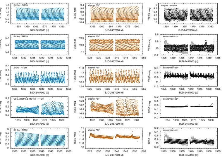
Figure 2. Comparison of thefitshdifferential-imaging aperture photometry (left row) with theeleanorphotometries. Center:
PSF fitting; right: raw (grey) and corrected (black) pixel aperture photometry. From top to bottom, three relatively bright stars from each subclass (RRab, RRc, RRd); a faint RR Lyrae star; SX Dor, from a crowded region near the Large Magellanic Cloud (LMC). Plots are on the same scale in each row.
The light curves were then analyzed by several co- authors separately, using predominantly thePeriod04 software (Lenz & Breger 2005) to identify pulsation peri- ods, harmonics and various other frequency components in the data. Temporal variations in the Fourier ampli- tudes and phases were also investigated.
2.3. Comparison with eleanor photometry The eleanor open-source software tool was devel- oped byFeinstein et al. (2019) to produce light curves from the TESS FFI data. The software is capable to do pixel aperture and PSF photometry, and decorrelat- ing systematics and co-trending signals from the light curves. We tested the performance of eleanor on a small selection of RR Lyrae stars. Classical correction methods, such as regressing the photometry against po- sition changes, are difficult to apply to RR Lyrae stars since the high-amplitude and rapidly-changing signal often overwhelms the comparatively smaller systemat-
ics. We found that the simple pixel-photometry light curves, corrected for pixel position-related changes (the CORR FLUX photometry), are of inferior quality com- pared to our results, as shown in Fig.2. This result was not unexpected as multiple correction methods devel- oped for general use in the K2 mission fared even worse when applied to RR Lyrae stars (Plachy et al. 2019).
In contrast, the PSF photometry produced by eleanor, which fits a two-dimensional Gaussian func- tion as PSF model to each frame, usually resulted in light curves that matched the quality of our data. This was true even for faint targets—down to 16 mag stars—
as long as the star was well separated. One example is CSS J233140.8–113458, shown in the fourth row of Fig2. Blending and nearby stars, however, can confuse the algorithm and may result in a poor light curve: this happened to SX Dor, which is in front of the outskirts of the LMC (last row of Fig 2). We concluded that limiting the size of the image cutout to exclude other
sources can be beneficial but the code requires a min- imum size of 9×9 px image for a reliable fit. We also observed differences between the average brightness and pulsation amplitude values produced by eleanor and our code: theeleanorlight curves are usually, but not always, fainter by up to 0.3 mag, or 33% in mean flux.
Lower mean flux suggests that the background level may be overestimated in the PSF photometry. This again highlights the difficulties caused by crowding and blending in the TESS images.
3. RESULTS
In this section we present various results obtained from the TESS light curves and Gaia measurements.
First we study the kinematics of the targets, and clas- sify the stars based on their absolute brightness, color and light curve shape information to create a clean RR Lyrae sample. We then study how accurately can we identify the Blazhko effect in the relatively short TESS light curves. We also evaluate the mode content of each light curve, and compare those results to earlier findings.
3.1. Kinematics
We searched for available radial velocities (RVs) for the selected RR Lyrae stars and found data for 57 tar- gets inGaia EDR3, in the Radial Velocity Experiment (RAVE,Steinmetz et al. 2020), in the Galactic Archaeol- ogy with HERMES Survey (GALAH DR3,Buder et al.
2021), and in the observations byLayden (1994). The Gaia, GALAH and RAVE surveys do not take into ac- count stellar pulsation in their radial velocity measure- ments, hence their values can be off by up≈75 km s−1 based on Eq. 1 in Liu (1991) and a projection factor of 1.37 (the ratio between intrinsic pulsation velocities and disk-averaged RVs: value fromSesar 2012). On the other hand, radial velocities derived by Layden (1994) take into account stellar pulsation and they report errors of order 15 km s−1. Multiple stars in our sample have radial velocities both in theGaia EDR3 and in theLay- den (1994) catalogues, and the difference between the two ranges from 10 km s−1 to 30 km s−1. Therefore we assumed a conservative error of 75 km s−1 on theGaia, GALAH and RAVE RVs.
We did not attempt to phase RV values for stars that are present in multiple databases: while this could, in principle, help us to determine the systemic velocity of the star more accurately, the phasing of multiple RV measurements may not be a trivial task. The alignment of these data would be affected not only by unknown phase shifts and possible modulation present in the pul- sation, but also by the fact that different surveys use different spectral lines that sample regions with differ- ent kinematics in the atmosphere (Braga et al. 2021).
0 100 200 300 400
-500 -400 -300 -200 -100 0 100
Halo
Thick disk
√(U2+W2) (km/s)
V(km/s)
Thin disk
Figure 3. Toomre diagram of 42 stars from our sample.
Black dots are halo RR Lyrae stars, blue squares are variables that may be members ofGaia-Enceladus structure according to Prudil et al. (2020). Dashed lines mark constant total space velocities while green lines show the approximate thin–
thick disk and disk–halo boundaries. The red crosses are two non-pulsating stars we identify in Section3.2.
Further, some databases do not provide precise times of measurement.
We used thegaiadr3 zeropointsoftware to correct for the zero point offset present in theGaia EDR3 par- allaxes (Lindegren et al. 2021a,b). We note that almost all RVs in Gaia DR2 are propagated into EDR3 un- changed, with the exception of the most discrepant val- ues in DR2, which were removed from the new catalog (Soubiran et al. 2018).
We then computed the full 6D orbital solution of the stars using the Gaia EDR3 proper motions and par- allaxes in concert with collected radial velocities using the galpy library (Bovy 2015). The whole calcula- tion was performed through a Monte Carlo error anal- ysis with varying the proper motions, parallaxes, and radial velocities within their errors. Uncertainties and covariances among all parameters were taken into ac- count in calculating the velocity uncertainties. The fi- nal values and their errors were taken as the medians and absolute median deviations from the generated dis- tributions. We corrected for the solar motion with re- spect to the local standard of rest with the velocities (U, V, W) = (11.1,12.24,7.25) km s−1, where the U component is defined pointing towards the anticenter direction (Sch¨onrich et al. 2010; Sch¨onrich 2012). We used z = 20.8±0.3 pc and r = 8.122±0.031 kpc for the solar position above the plane and the distance to the Galactic center, respectively (Bennett & Bovy 2019;Gravity Collaboration et al. 2018). The resulting velocity components U, V and W are the rectangular Heliocentric velocity components.
Moln´ar et al.
Stars spread out in Fig. 3 that effectively shows or- bital energy and angular momentum compared to the Local Standard of Rest. Stars with high total velocities, above 180–200 km s−1 are halo members. Stars with velocities below that are part of the disk, with the thin–
thick boundary being at around 46 km s−1(Bensby et al.
2003;Buder et al. 2019). While most of the stars in the sample are either part of the halo or the thick disk, two objects, marked red, are close to zero, i.e., they clearly belong to the thin disk and follow galactic orbits similar to that of the Sun. We later show that these stars are in fact not pulsating stars.
We crossmatched our list of objects with the 314 ob- jects studied by Prudil et al. (2020). Since Sectors 1–
2 are far from the Galactic plane, we found no objects that were identified as possible thin-disk RR Lyrae stars.
However, four of our targets (UW Gru, VW Scl, YY Tuc and XZ Mic) are potentially members of the Gaia- Enceladus structure, also known as the Gaia Sausage, the remnant of a galaxy merged into the Milky Way (Helmi et al. 2018). This sample is currently too small to analyze separately but highlights the fact that we will be able to use TESS to study different RR Lyrae populations.
3.2. Classification
The stars selected for this study have been classified as RR Lyrae at least once already by prior studies. How- ever, these classifications are sometimes based on obser- vations of limited quality and/or quantity. We there- fore verified the classifications based on the TESS light curves, complemented by Gaia EDR3 brightness and parallax data (Gaia Collaboration et al. 2021).
3.2.1. Absolute magnitudes and distances
We computed the absolute magnitudes in the Gaia EDR3 G, GBP and GRP bands, using the geometric Gaia EDR3 distances calculated byBailer-Jones et al.
(2021), and correcting for extinction with themwdust code (Bovy et al. 2016). We used the combined maps created by Bovy et al. (2016). This method provided good separation between the intrinsically fainter rota- tional variables and binaries and the brighter, evolved HB stars where we expect RR Lyrae variables to appear.
The calculated absolute brightness values are plotted in Fig.4, along with the distribution of the absorption co- efficients in the sky. We also calculated absolute magni- tudes in theV, J, H andK bands, based on the bright- ness values listed in the SIMBAD database for each star (Wenger et al. 2000). GeometricGaia distances for RR Lyrae stars have been verified previously for the DR2 data byHernitschek et al.(2019). They found that they are accurate to about 5 kpc, but lose accuracy beyond
about 10 kpc, at which point they become dominated by the distance prior used byBailer-Jones et al.(2018). We can therefore expect the EDR3 distances for our sample, which only extends to 5 kpc, to be accurate as well.
The MG brightness of most of the stars is between 1.5 and 0.0 mag, where we expect horizontal-branch stars to cluster (Gaia Collaboration et al. 2018b). Six stars fall clearly below this range. The variations of the two faintest (marked with blue plus signs), ASAS J212045–5649.2 and ASAS J225559–2709.9, look super- ficially like RR Lyrae-type pulsation: these are likely rotational and/or ellipsoidal variables. Four more are cataloged as RR Lyrae stars but the TESS light curves make it clear that these are eclipsing binaries (blue cross signs). These are, in decreasing absolute brightness:
CRTS J215543.7-500050, AZ Pic, UW Dor and UY Scl.
We note that UY Scl has been listed previously as a possible binary RR Lyrae based on its large proper mo- tion anomaly in DR2 (Kervella et al. 2019b). We cal- culated velocity components for two of these six targets in Sect.3.1. ASAS J212045–5649.2 and UY Scl are the two red crosses in Fig.3, closest to zero, indicating that they are part of the thin disk.
Three other stars stand out due to high absorption co- efficient values (AG = 1.4, 2.6 and 3.0 mag, for OGLE LMC–RRLYR–03497 (also known as SW Dor), OGLE BRIGHT–LMC–RRLYR–3 and ASAS J045426–6626.2, respectively): all three lie in the direction of the LMC, as the sky map in Fig.4indicates. OGLE BRIGHT–LMC–
RRLYR–3 was newly identified in the OGLE–III LMC Shallow Survey as a Galactic RR Lyrae: it is known as OGLE LMC–RRLYR–28980 in their main catalog (Ulaczyk et al. 2013). Since all three stars are clearly nearby stars that are in the foreground of the LMC, these extinction corrections appear to be excessive. To test this we then calculated the interstellar absorption using the SFD dust maps instead (Schlafly & Finkbeiner 2011): for these three stars the SFD map gave about 0.7–1.5 mag smaller absorption but two of the three still remained overluminuos.
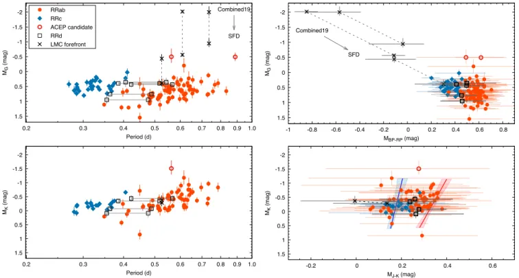
3.2.2. Period-luminosity relations and colors With the pulsation periods from the TESS light curves in hand, we created the period-luminosity plot of our TESS first light sample inMGandMKbands, as shown in the left panels of Fig. 5. With this sample size the slopes of the PL relations are not entirely apparent, es- pecially for the RRc stars, but the increase in bright- ness with the period can be seen. K-band brightness is much less sensitive to interstellar extinction than shorter wavelengths, limiting the spread of the PL relation, al- though for RR Lyrae stars the spread of the PL rela-
-3
-2
-1
0 1 2 3 4 5 6 7
8 0.1 1 10
rotation and binaries RR Lyrae
LMC foreground
BRIGHT-LMC-RRLYR-3
LMC-RRLYR-03497 ASAS J045426-6626.2
MG(mag)
d(kpc) RRab
RRc RRd LMC fg ACEP?
EB EB/ROT?
-3
-2
-1
0 1 2 3 4 5 6 7
8 0.1 1 10 0
0.1 0.2 0.3 0.4 0.5 0.6 0.7 0.8 0.9 1
1.1 1.2 1.3 1.4 1.5
AG(mag)
MC MC MC MC
MC 270° 180°
0°90°
180°
+36°
-36°
+90°
-90°
RA Dec MC
Figure 4. Main: theGaia EDR3MG absolute magnitudes and distances of the sample, color-coded with theAGabsorption coefficients calculated withmwdust. The diagonal line and light-grey area below it mark the approximate brightness cut of the sample. Large crosses mark eclipsing stars that we were able to classify based on light curve shapes. The large pluses at the bottom are two stars where the light curve shape was not decisive but their positions clearly rule them out. Different extinction corrections for the three LMC foreground stars are connected with the dashed lines. Insert: map of the targets with and the AGabsorption coefficients in the EDR3G band. The position of the Magellanic Clouds is marked with the arrow.
tion is largely driven by metallicity (Catelan et al. 2004;
Layden et al. 2019;Bhardwaj et al. 2021;Gilligan et al.
2021). Furthermore, not all stars have their K bright- ness measured (here, 32 of the 118 targets are missing from the lower plots), and even when they do, single- epoch measurements may not represent mean brightness values.
For RRd stars both of their periods are indicated by the black empty squares. Two of the three over- corrected stars, ASAS J045426–6626.2 and BRIGHT–
LMC–RRLYR–3, stand out with either correction meth- ods, but the third, LMC–RRLYR–03497, moves into the RRab locus with the lower, SFD-based correction.
We also calculated the extinction-corrected EDR3 GBP−GRPandJ−Kcolors for every star. In the color- magnitude diagrams (CMDs, right panels of Fig.5) the three stars that are in front of the LMC are clearly shifted bluewards (black crosses), confirming that they are over-corrected for interstellar extinction. Tracing them back along the reddening vector to the expected colors indicate that they would be part of the RR Lyrae group. We note that the star LMC–RRLYR–03497—
which apparently falls into the RRc group with the SFD
correction—is in fact an RRab pulsator, as indicated by its period and light curve shape. We therefore con- clude that both the Combined19 dust map ofBovy et al.
(2016) and the SFD map overestimate the required ex- tinction for stars that are directly in front of the LMC. In the near-infrared CMD (lower right panel of Fig.5), we were able to overlay the theoretical blue and red edges of the instability strip, as calculated byMarconi et al.
(2015). In this CMD the RRab and RRc stars appear to be mixed in color, likely because neither magnitudes represent the mean brightness. However, multiple stars fall outside of the first overtone blue edge, but almost none are redder than the fundamental mode red edge.
We identified two stars that have the expected colors but still appear to be more luminous than the bulk of the sample: ASAS J221052–5508.0 (P = 0.887 d) and SX PsA (P = 0.563 d) are both above the RR Lyrae locus, although only marginally in the latter case. K brightness is only available for the latter, but this also appears to exceed the brightnesses of the rest of the stars. We consider the possibility that these are anoma- lous Cepheids in Sect. 3.2.4. The intrinsically faintest RR Lyrae star in the sample is XZ Mic.
Moln´ar et al.
-2 -1.5 -1 -0.5 0 0.5 1 1.5
0.2 0.3 0.4 0.5 0.6 0.7 0.8 0.9 1.0
Combined19
SFD
MG(mag)
Period(d) RRab
RRc ACEPcandidate RRd LMC forefront
-2 -1.5 -1 -0.5 0 0.5 1 1.5
-1 -0.8 -0.6 -0.4 -0.2 0 0.2 0.4 0.6 0.8
Combined19
SFD
MG(mag)
MBP-RP(mag) -2
-1.5 -1 -0.5 0 0.5 1 1.5
0.2 0.3 0.4 0.5 0.6 0.7 0.8 0.9 1.0
MK(mag)
Period(d)
-2 -1.5 -1 -0.5 0 0.5 1 1.5
-0.2 0 0.2 0.4 0.6
MK(mag)
MJ-K(mag)
Figure 5. Left: period-luminosity relation of the sample. Brightness is inMG(top) andMK (bottom) absolute magnitudes.
RRab and RRc stars are represented with blue diamonds and red dots, respectively. For RRd stars (black empty rectangles) we marked both periods. The two anomalous Cepheid (ACEP) candidates are marked with empty circles. Stars with erroneous extinction correction are marked with black crosses. Right: distribution of the sample in the absoluteGaia andJ–K (bottom) color-magnitude planes: here we marked the blue and red edges of the instability strip, as calculated byMarconi et al.(2015), with the blue and red solid lines. Differences between the two extinction corrections are indicated with dashed lines for the three LMC foreground stars.
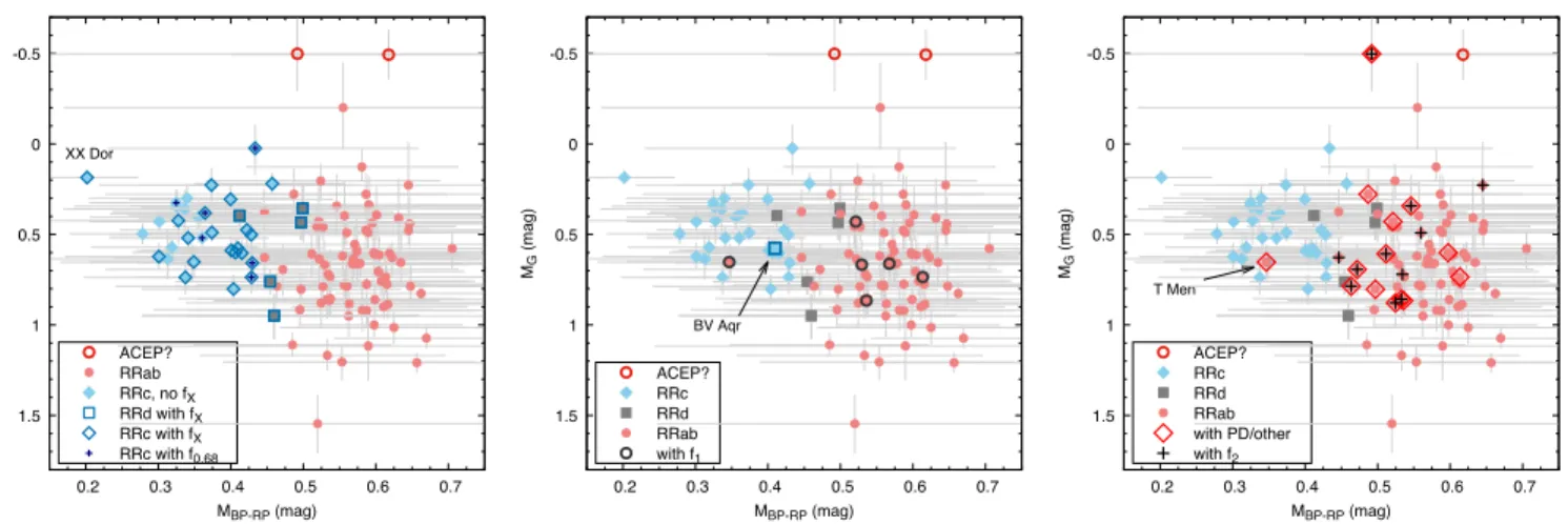
The color-magnitude diagram also shows that the RRc and RRab subclasses (as determined in the next sec- tion) clearly cluster towards the blue and red sides of the group in theGaia passbands, with the RRd stars falling in the middle. The apparent color values themselves are typically precise to less than 0.05 mag, which would make color-based classification possible, but extinction correction imparts further uncertainties typically in the range of 0.1–0.3 mag. This means that although the RRc and RRab data points clearly separate in theGaia CMD (but not in the near-infrared one), their uncer- tainty ranges overlap, which prevent us from using color as a primary classification metric.
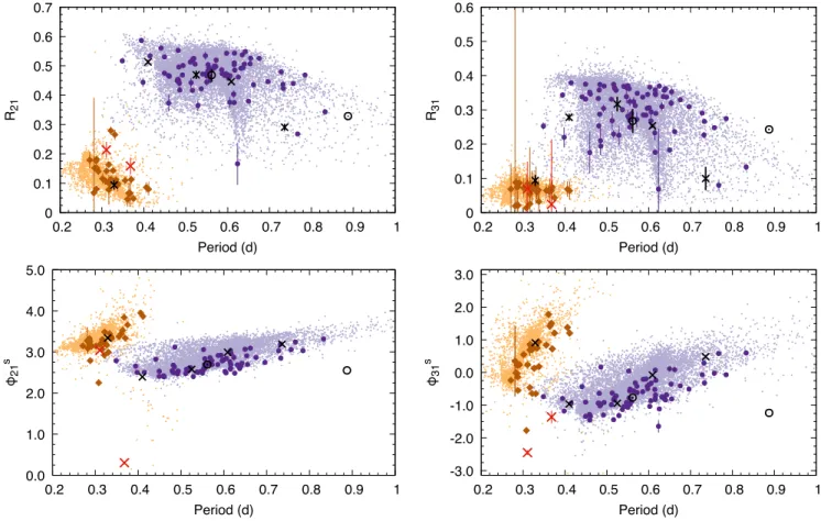
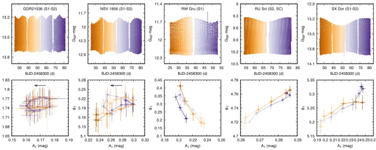
3.2.3. Relative Fourier parameters
With the Fourier parameters of the main pulsation pe- riods and harmonics fitted, we can compute the relative Fourier parameters Ri1 = Ai/A1 and φi1 = φi −i φ1
to classify the stars based on their light curve shapes (Simon & Teays 1982). We use sine-based Fourier se- ries in the form of m = m0+P
iAi sin(2π if0t+φi), where m0 is the average brightness,f0 is the dominant pulsation frequency, Ai and φi are the amplitudes and
phases of each harmonic and i is the harmonic order.
This method does not necessarily separate non-pulsating stars from pulsating stars if their variations look simi- lar but it is capable of differentiating between pulsation modes among the RR Lyrae stars. We compared the TESS results to those of the OGLE stars as a reference, as shown in Fig. 6. Since the TESS passband is cen- tered on theIband, we expect only minor differences in the distribution of the Fourier parameters of the OGLE I and TESS measurements. The R parameters indeed show very good agreement for both the RRab and RRc loci, but we see differences in theφparameters, with the TESS data clustering at slightly lower values than the OGLE data. A systematic shift between theφ31param- eters in the I band and TESS pass-band light curves indicate that the we cannot adopt existing relations to calculate the photometric metallicities (Skowron et al.
2016). We estimate the shifts in phase difference to be φ21,I−φ21,TESS≈0.15 andφ31,I−φ31,TESS≈0.25 rad.
Calibration of photometric [Fe/H] indices for the TESS passband will be discussed in a separate paper.
We indicated the three LMC foreground stars with black crosses. Each appears within the RRab loci of
0 0.1 0.2 0.3 0.4 0.5 0.6 0.7
0.2 0.3 0.4 0.5 0.6 0.7 0.8 0.9 1
R21
Period(d)
0 0.1 0.2 0.3 0.4 0.5 0.6
0.2 0.3 0.4 0.5 0.6 0.7 0.8 0.9 1
R31
Period(d)
0.0 1.0 2.0 3.0 4.0 5.0
0.2 0.3 0.4 0.5 0.6 0.7 0.8 0.9 1
φ21s
Period(d)
-3.0 -2.0 -1.0 0.0 1.0 2.0 3.0
0.2 0.3 0.4 0.5 0.6 0.7 0.8 0.9 1
φ31s
Period(d)
Figure 6. Relative Fourier parameters Ri1 and φi1 of the TESS first light sample (large symbols), overlaid on the OGLE I-band values (dots). Orange and purple points mark RRc and RRab stars. The two empty circles are the anomalous Cepheid candidates, the three black crosses in the RRab group are the three LMC foreground stars. The two red crosses in the RRc group are two false positive, non-pulsating stars.
each parameter, confirming that these are RRab stars and that their intrinsic luminosities and colors must be lower than what we computed with the mwdust code.
We also indicate the anomalous Cepheid candidates with black circles.
Although we removed obvious eclipsing binary and rotational variable light curves from the sample prior to classification, the distance-luminosity and period- luminosity plots in Fig. 4 revealed two further dwarf stars in the sample (blue plus signs in Fig. 4). Their Fourier parameters are at least in marginal agreement with the distribution of RRc stars: the Ri1 parameters agree, the φ21 is inconclusive since at longer overtone periods bona fide RRc stars span the whole range, and only theφ31 value appears to be discrepant. Therefore, classification of these two stars would have remained ambiguous from the light curve shapes alone, and the accurate parallax data were necessary to exclude them from the sample.
Based on the absolute brightness, light curve shape and period ratio information, we identified 82 RRab, 31
RRc, and 5 RRd stars among the selected stars. This amounts to 118 RR Lyrae targets in total.
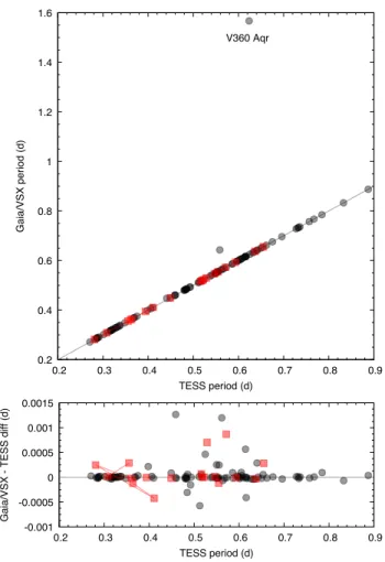
Finally, we compared the pulsation periods we ob- tained with those in the Gaia DR2 catalog (specifi- cally, the RR Lyrae and Cepheid periods calculated by Clementini et al. (2019)). Of the 118+2 stars, 21 have not been identified as either type of variable: in those cases we queried the International Variable Star Index (VSX). As Fig.7 shows, almost allGaia or VSX periods agree with those we derived from the TESS light curves. The most distant point is V360 Aqr, an RRab that was classified as a Type II Cepheid (T2CEP) by the Gaia algorithm. A smaller but clear differ- ence is observed for LMC–RRLYR–23457. The rest of the stars show only small differences, although in multiple cases such differences exceed the uncertain- ties of both the TESS and Gaia periods. Most of the stars have been correctly classified in Gaia: aside from V360 Aqr, only four more stars are erroneous. SU Hyi, the shortest-period RRab star, and an double-mode star, Gaia DR2 6529889228241771264 were classified as RRC stars, whereas two RRab stars, AE Tuc and ASAS
Moln´ar et al.
0.2 0.4 0.6 0.8 1 1.2 1.4 1.6
0.2 0.3 0.4 0.5 0.6 0.7 0.8 0.9
V360 Aqr
Gaia/VSXperiod(d)
TESS period (d)
-0.001 -0.0005 0 0.0005 0.001 0.0015
0.2 0.3 0.4 0.5 0.6 0.7 0.8 0.9
Gaia/VSX-TESSdiff(d)
TESSperiod(d)
Figure 7. Comparison of the pulsation periods we derived from the TESS light curves and those calculated from the GaiaDR2 epoch photometry (grey) or present in VSX (red).
Stars where two periods were identified only by either TESS orGaiaare connected with lines. The lower panel shows the difference values. Uncertainties are smaller than the sym- bols.
J215601–6129.2 were classified as RRD stars in theGaia notation. These statistics agree with earlier validation tests based onKepler data, which found that class mis- matches in the Gaia classification are rare among the bright RR Lyrae stars (Moln´ar et al. 2018).
3.2.4. Anomalous Cepheid candidates
In addition to the 118 RR Lyrae stars, we also found two over-luminous outliers, SX PsA and ASAS J221052- 5508.0, both at MG =−0.5 mag. The higher absolute brightness and long period (P = 0.887 d) suggest that ASAS J221052-5508.0 is an anomalous Cepheid (ACEP) star rather than an RR Lyrae. The classification of SX PsA is more uncertain, given its shorter period. We compared the two stars’ Fourier parameters to those of the OGLE ACEPs in Fig. 8, and they both fit into the fundamental-mode ACEP locus, although the latter is at the short period end of the distribution. At the
0 0.1 0.2 0.3 0.4 0.5 0.6 0.7
0.4 0.6 0.8 1 1.2 1.4
R21
Period (d)
0 0.1 0.2 0.3 0.4 0.5 0.6
0.4 0.6 0.8 1 1.2 1.4
SX PsA ASAS
R31
Period (d)
0.0 1.0 2.0 3.0 4.0 5.0
0.4 0.6 0.8 1 1.2 1.4 φ21s
Period(d)
-3.0 -2.0 -1.0 0.0 1.0 2.0 3.0
0.4 0.6 0.8 1 1.2 1.4 φ31s
Period(d)
Figure 8. Relative Fourier parameters of the two anoma- lous Cepheid candidates, compared to the OGLE anomalous Cepheid samples (Soszy´nski et al. 2015,2020).
shortest periods, however, the distribution of RR Lyrae and ACEP Fourier parameters strongly overlap, and as Fig.6 shows, SX PsA fits into the RRab locus as well.
We propose that the more luminous one, ASAS J221052–5508.0 is indeed a newly identified, Galactic anomalous Cepheid. The classification of SX PsA is less certain, and we consider it an ACEP candidate. As SX PsA also displays strong amplitude modulation, this would be another ACEP star showing the Blazhko effect, after the identification of the first modulated ACEP can- didate in the K2 observations by Plachy et al. (2019).
Although we prefer the ACEP classification, SX PsA could possibly be an unusually luminous RR Lyrae star, too.
Unfortunately, most anomalous Cepheids identified in Gaia DR2 are too far away to have accurate geomet- ric parallaxes. We therefore do not yet have a well- calibrated PL relation for Galactic ACEP stars, and too few have been studied so far with TESS (Clementini et al. 2019; Plachy et al. 2021). The importance of dis- tance determination was also highlighted byBraga et al.
(2020), who showed that short-period ACEP and Type II Cepheids can overlap in period with long-period RR Lyrae stars. Period itself is therefore not a unique clas- sifier, and a reliable separation of Galactic short-period ACEP stars from long-period RR Lyrae stars will re- quire accurate light curve shape information, distances and colors. Once we can separate these with confidence, we will be able to construct a PL relation for Galactic ACEP stars, too.
3.3. The Blazhko effect
Modulation has been detected in all subtypes of RR Lyrae stars, even in RRd stars (see, e.g., Smolec et al. 2015; Plachy et al. 2017b; Carrell et al. 2021).
Amplitude and phase modulation in RR Lyrae stars happen over periods extending from a few days to years, therefore one or two Sectors’ worth of data are not well- suited to studying the Blazhko effect. Nevertheless, we were able to identify the signs of amplitude and phase changes in several stars. Although we cannot rule out the possibility of non-cyclic amplitude and phase shifts in RR Lyrae stars over short time scales, evidence for such events is scant in long-term observations. We therefore consider contamination from non-Blazhko ob- jects to be negligible and classify all targets with smooth changes to the pulsation properties as Blazhko stars.
Currently the best hypothesis for the Blazhko effect is the non-linear mode resonances model (Buchler &
Koll´ath 2011; Koll´ath 2018). It agrees best with obser- vations; however, the model is based on amplitude equa- tion calculations, and the accurate reproduction of mod- ulated light curves in hydrodynamic simulations is still in its infancy (see, e.g., Moln´ar et al. 2012a; Smolec &
Moskalik 2012;Goldberg et al. 2020;Joyce et al. 2020).
3.3.1. What is the Blazhko effect – for an observer?
Since we do not have a universally accepted model for the Blazhko effect, we have noa prioriconstraints on the distributions and limits of the modulation periods and amplitudes. With the precision achieveable with Ke- pler and TESS, we can now detect millimagnitude-level modulations: however, we must ask whether we should label all quasi-periodic modulations as the Blazhko ef- fect. Moskalik et al.(2015), for example, stated that the small amplitude and phase fluctuations in the Kepler RRc stars do not resemble the classical picture of the (semi-)coherent modulations we know as the Blazhko effect. Similarly, Benk˝o et al. (2019) found that cycle- to-cycle variations inKeplerRRab stars can cause small side peaks, but the true incidence rate of quasi-periodic modulation is 51–55%. In contrast, the idea that all RR Lyrae stars are modulated was recently suggested by Kov´acs (2018), based on his processing of K2 data.
It is therefore important to test whether this hypothesis can be confirmed with the TESS sample.
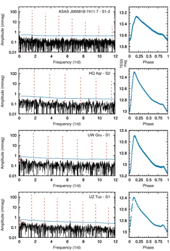
The classical Blazhko effect manifests itself as side- peaks around the pulsation frequency and its harmonics in frequency space. In principle, searching for signifi- cant sidepeaks is a straightforward exercise. However, contamination from stellar or instrumental sources, as well as systematics introduced by the photometric and post-processing pipelines can inject variations mimick-
ing small modulations. Slow changes in the average flux, for example, can be caused both by changes in the amount of captured flux (e.g., intra- and interpixel sensitivity changes) or by contamination from a sepa- rate source, or both, but they affect the flux amplitude differently. Choices to correct these via scaling and/or subtracting flux can be a degenerate problem. Improper handling of systematics and contamination may either introduce artificial amplitude changes that appear as sidepeaks in the frequency spectra, or remove slow vari- ations intrinsic to the star. The same issues were found to affect some of the K2 light curves as well (Plachy et al. 2017a, 2019). In the TESS data we found that systematics tend to generate sidepeaks surrounding only the pulsation frequency or very few harmonics, whereas Blazhko stars have a clear series of sidepeaks along the harmonics.
Furthermore, theKeplerdata demonstrated that stars where no coherent amplitude and phase variation were detected still showed irregular amplitude and phase fluc- tuations, similar to those seen in Cepheids (Benk˝o et al.
2019). While over long timescales this manifests as red noise around the main harmonic series, over the much shorter TESS observations, stochastic variations can conceivably appear as a single or a few significant frequency components in some cases.
Another problem we encountered stems from the fact that the amplitude of the main frequency peak is sev- eral orders of magnitude larger than the photometric noise level. This can cause some algorithms to be able to reach sufficiently small pre-set residual levels even with a slightly offset frequency fit. This results in an apparent phase shift between the data and the fit which can be mistaken for intrinsic modulation. We noticed this behavior when fitting RRc stars inPeriod04. We therefore double-checked all stars where an apparent lin- ear phase shift was observed without any counterpart in the pulsation amplitude and then adjusted the pulsation frequency manually to minimize the phase shift over the length of the data. Here we also note that nearly linear phase shifts in short data sets can be caused by a very long modulation cycle as well, but we cannot separate those based on the TESS data alone, if no significant amplitude change is detectable alongside with them.
Therefore we refrain from claiming that any star that shows sidepeaks to the main pulsation frequency and its harmonics must automatically be a Blazhko star and set more strict rules. However, in lieu of a detailed model, reasons either for or against such distinction are based on phenomenological and methodological considerations alone.