arXiv:1806.01546v1 [astro-ph.SR] 5 Jun 2018

(1)

arXiv:1806.01546v1 [astro-ph.SR] 5 Jun 2018

SPOTS, FLARES, ACCRETION, AND OBSCURATION IN THE PRE-MAIN SEQUENCE BINARY DQ TAU

A. K´´ ospál,^{1, 2} P. Ábrahám,¹ G. Zsidi,¹ K. Vida,¹ R. Szabó,¹ A. Moór,¹ and A. Pál¹

1Konkoly Observatory, Research Centre for Astronomy and Earth Sciences, Hungarian Academy of Sciences, Konkoly-Thege Mikl´os ´ut 15-17, 1121 Budapest, Hungary

2Max Planck Institute for Astronomy, K¨onigstuhl 17, 69117 Heidelberg, Germany

(Received 2018 February 25; Revised 2018 May 3; Accepted 2018 June 4) Submitted to ApJ

ABSTRACT

DQ Tau is a young low-mass spectroscopic binary, consisting of two almost equal-mass stars on a 15.8 d period surrounded by a circumbinary disk. Here, we analyze DQ Tau’s light curves obtained by Kepler K2, the Spitzer Space Telescope, and ground-based facilities. We observed variability phenomena, including rotational modulation by stellar spots, brief brightening events due to stellar flares, long brightening events around periastron due to increased accretion, and short dips due to brief circumstellar obscuration. The rotational modulation appears as sinusoidal variation with a period of 3.017 d. In our model this is caused by extended stellar spots 400 K colder than the stellar effective temperature. During our 80-day-long monitoring we detected 40 stellar flares with energies up to 1.2×10³⁵erg and duration of a few hours. The flare profiles closely resemble those in older late-type stars, and their occurrence does not correlate with either the rotational or the orbital period. We observe elevated accretion rate up to 5×10⁻⁸M⊙yr⁻¹ around each periastron. OurSpitzerdata suggests that the increased accretion luminosity heats up the inner part of the circumbinary disk temporarily by about 100 K. We found an inner disk radius of 0.13 au, significantly smaller than expected from dynamical modeling of circumbinary disks. Interestingly, the inner edge of the disk is in corotation with the binary’s orbit. DQ Tau also shows short dips of<0.1 mag in its light curve, reminiscent of the well-known “dipper phenomenon” observed in many low-mass young stars.

Keywords: stars: pre-main sequence — stars: circumstellar matter — stars: individual(DQ Tau)

kospal@konkoly.hu

(2)

1. INTRODUCTION

Pre-main sequence stars are intimately linked with their circumstellar material. This relationship manifests in a variety of phenomena that makes young stars highly variable at a wide range of wavelengths. The photometric variability of young stars can be traced back to four main origins: variable accretion, rotational modulation due to hot or cold stellar spots, variable line-of-sight extinction, and stellar flares.

According to the magnetospheric accretion model for T Tauri stars (e.g.,Hartmann et al. 1994), the circumstellar disk is truncated by the star’s magnetic field and material is channeled through accretion columns onto the star. Unsteady accretion leads to a variable accretion rate, which may cause variability at optical wavelengths by up to a few mangitudes on timescales as short as a few hours, typically observed in classical T Tauri stars (e.g., Herbst et al. 1994;

Gullbring 1994; Wood et al. 1996; Stassun & Wood 1999; Romanova et al. 2008). Hot spots form at the footpoints of the accretion columns, where shocks form due to the conversion of kinetic energy to heat (e.g.

Dodin 2015).

Due to their strong magnetic fields (on the order of a few kG on the stellar surface), low-mass, late-type young stars may have extensive dark spots on their surface, which are the scaled-up versions of sunspots. Spots on very active young stars may cover more than half of the star’s surface and are the main cause of variability in weak-line T Tauri stars, causing variability on a few days timescale with amplitudes up to a few tenths of a magnitude (Fernandez & Miranda 1998;Lehtinen et al. 2016).

While the period of variability due to dark starspots is very stable, the exact shape of the light curve can change in a few weeks (Herbst et al. 1994).

Some low-mass pre-main sequence stars show irregular or periodic fadings attributed to variable circumstellar extincion, called “dipper phenomenon” (e.g.

Cody et al. 2014, and references therein). In these cases, clumps of dusty material lifted from the disk’s inner edge (Bodman et al. 2017) or a warp in the inner disk (Bouvier et al. 1999) temporarily obscure part of the starlight.

Finally, pre-main sequence stars are known to ex- hibit flares, predominantly in X-rays (Stelzer et al.

2000; Feigelson et al. 2002; Favata et al. 2005), but in some cases also in the UV and optical/white-light (Rydgren & Vrba 1983;Vrba et al. 1988; Stassun et al.

2006; Frasca et al. 2009). Analogous to solar flares, these events are probably the consequences of energy released in a magnetic reconnection event above an active region on the stellar surface.

While some of the listed effects causing photometric variability have been observed in different young stars, no object has been known to display all of them, possi- bly due to observational limitations. However, the second mission of theKeplerspacecraft (K2) provided very precise photometry for many young stars in the Taurus star forming region in 2017. One of them, DQ Tau, is an extraordinary close binary system with a circumbinary disk, which shows very complex variability pat- terns. With the aim of determining the physical origin of DQ Tau’s variability and disentangle the different effects, here we analyze the very high cadence (about 1 minute) uninterrupted 80-day-long white light monitoring of this system obtained during the K2 mission.

We complemented the K2 data with multifilter optical photometry to determine color changes and mid-infrared observations with theSpitzer Space Telescope to study the response of the inner disk emission to the variable irradiation coming from the stellar surface.

In Section2we introduce our target in detail. In Sec.3 we present our observations, then we describe the im- mediate results on the rotational, flare, and accretion variability in Section 4. In Section 5 we interpet the periodic results using a spot model, and put into con- text the detected flares by comparing them with similar flares on M-type stars. After analyzing the energetics and morphology of the brightening of the system near periastron and discussing the possible reasons for the observed variable extinction, we summarize our results in Section6.

2. OUR TARGET

DQ Tau is a pre-main sequence binary, consisting of two almost identical classical T Tauri-type stars. The system is located in the Taurus star forming region at a distance of 140 pc¹ (Kenyon et al. 1994). Based on a recent comprehensive study ofCzekala et al.(2016), the stars orbit each other in an eccentric orbit (a=28.96R⊙, e=0.568), with a period of 15.80158±0.00066 d. At periastron they approach each other within 12.5R⊙

(0.06 au), while at apastron their separation is 45.4R⊙

(0.21 au). The masses and effective temperatures of the primary and the secondary are M¹ = 0.63±0.13M⊙, T¹=3700 K, andM² = 0.59±0.13M⊙,T²=3500 K, respectively. The binary is surrounded by a circumbinary protoplanetary disk, from which gas and dust are

1 The parallax from the Gaia DR2 catalog, converted to unbi- ased, correct distances and uncertainties usingBailer-Jones et al.

(2018), implies a larger distance value of 196.4±2.0 pc. However, since Gaia parallaxes of binary stars might change in later data releases, and since we prefer to keep our results comparable with earlier literature, we use 140 pc throughout this paper.

(3)

still accreting onto the stars. ALMA observations of (Czekala et al. 2016) imply that the system is seen close to pole-on (i=22^◦).

DQ Tau has been known for its quasi-periodic optical variability, brightening by up to 0.8 mag around periastron epochs (e.g., Mathieu et al. 1997; Salter et al.

2010; Tofflemire et al. 2017). One hypothesis to explain the observed light changes is periodically modulated accretion from the circumbinary disk onto the star. Hydrodynamical modeling of circumbinary disks (e.g.,Artymowicz & Lubow 1996) predicts a gap in the inner part of the system cleared by the binary’s motion. These models, however, also predict a temporary stream of accreting material accross this gap, synchro- nized with the orbital motion of the stars. This phenomenon is called pulsed accretion. The interpretation of the brightenings in DQ Tau as accretion events is en- forced by the detection of broad and variable Hαemis- sion (e.g.,Mathieu et al. 1997).

Periodic occurrence of millimeter flares (Salter et al.

2008,2010) and elevated X-ray activity near periastron (Getman et al. 2011, 2016) highlighted the importance of the binary’s magnetic field. At the periastron passage, when the stars approach each other, their magnetic fields collide, resulting in high-energy flares. The periodically merging and separating magnetospheres probably cre- ate a special environment for mass accretion, which has never been theoretically or numerically studied. This raises the possibility that the periastron brightenings are due to a combination of magnetic and dynamic effects.

Because DQ Tau is the prime example for pulsed accretion, it is important to clarify the physical origin of the brightness variations. In order to decide on the un- derlying processes,Tofflemire et al. (2017) performed a long-term multifilter optical monitoring of the system, covering ten orbital periods. They detected the periastron brightenings, and also showed hints for apastron brightness increases. Based on the morphology of the brightness peaks and on the energetics of the events (compared to typical flare profiles and activity of M- type main sequence stars), they concluded that the flux maxima close to periastron are related to temporary accretion from the circumbinary disk onto the stars. They also detected two magnetic flare-like events, but these were insufficient to explain the energetic brightenings around periastron.

3. OBSERVATIONS AND DATA REDUCTION DQ Tau was suggested as a target for theKepler K2 Campaign 13 in our proposal (proposal ID: GO13005, PI: Á. Kóspál). Observations started on 2017 March 8, and finished on 2017 May 27, providing an 80-day long

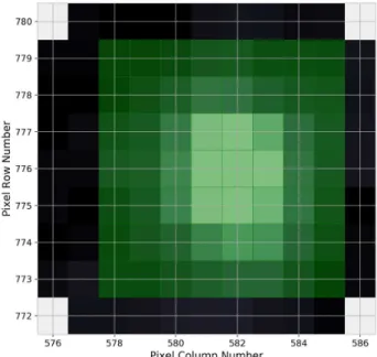
Figure 1. The large photometric aperture mask applied to DQ Tau. The black pixels were downloaded from the spacecraft, the star is shown by the lighter shades, while the mask we applied to measure the flux variation of the object is highlighted in green. This set of pixels corresponds to the beginning of Campaign 13.

uninterrupted monitoring of the white-light brightness of DQ Tau with a cadence of both 30 min (long cadence data) and 1 min (short cadence data).

Since during the K2 mission the spacecraft operates only with two reaction wheels, periodic thruster firings are necessary to maintain pointing. The drift due to the solar pressure and the subsequent correction maneuvers every few hours introduce systematic deviations in the K2 light curves. This can be (1) due to an inadequately chosen photometric mask, (2) because the star falls on pixels of varying sensitivity, and (3) also because of in- trapixel variations. According to the K2 C13 Data Re- lease Notes², the C13 pointing and roll behavior were within the limits of that seen in other K2 campaigns.

The maximum distance between the derived and nomi- nal positions for any target for C13 was well under the 3-pixel limit except for three (6–18 h long) periods with anomalous thruster firings: one at the very beginning of the Campaign, and two during the last 5 days of C13.

These data were discarded from further analysis. The smear correction error of Channel 74 mentioned in the

2https://keplerscience.arc.nasa.gov/k2-data-release-notes.html

#k2-campaign-13

(4)

Data Release Notes does not affect the data on our target.

In order to extract flux variations, we used the PyKE software package³ (Still & Barclay 2012). To sum the flux for the target, we employed a large aperture in order to accommodate shifts due to the telescope drift. We made an aperture file manually using the PyKEkepmask task, then the flux was obtained by the kepextract task. The mask we applied for DQ Tau is shown in Fig. 1. We followed the Extended Aperture Method (EAP, Moln´ar et al. in prep.), and used a large aperture, which provided comparable or better results (especially for large amplitude variations) than other pipelines and took care of any pointing systematics. We compared our extracted light curves to two such avail- able pipeline products, namely K2SFF (K2 Self-Flat- Fielding, Vanderburg & Johnson 2014) and EVEREST (EPIC Variability Extraction and Removal for Exo- planet Science Targets, Luger et al. 2016). We found a very good agreement (differences below 0.004 mag) between our light curve and the result of EVEREST.

There were larger differences (up to 0.12 mag) between our light curve and the result of K2SFF, but the K2SFF light curve is noisier and still contains some artifacts due to the spacecraft’s maneuvers every few hours. There- fore, we concluded that our method gives a reliable light curve for DQ Tau and no detrending is necessary.

To calibrate the K2 counts in physical units (erg s⁻¹ and Kp magnitude), we first constructed the spectral energy distribution (SED) of DQ Tau using photometry from the VizieR database. We then fitted a reddened stellar model fromCastelli & Kurucz (2004) to the optical data points, using AV = 1.5 mag (Tofflemire et al.

2017) and an effective temperature of 3600 K, the average of the two binary components’ temperatures (3500 K and 3700 K) as given byCzekala et al.(2016). The stellar photosphere model reproduced the observed SED very well in the 0.4–1.6µm wavelength range, while the target displayed infrared excess emission at wavelengths longer than about 1.6µm. We convolved the fitted photosphere model with the high resolution response function of Kepler and integrated it over frequency to obtain the flux of DQ Tau in the Kepler band. Finally, we multiplied the flux by 4πd² (using a distance of d=140 pc), and obtained a luminosity of 1.09×10³²erg s⁻¹. Similarly, we used the spectrum of Vega fromBohlin & Gilliland (2004), convolved it with Kepler’s response function, and integrated it over frequency to obtain Vega’s flux in the Kepler band. As-

3http://pyke.keplerscience.org/

suming that Vega’s magnitude is 0, the two fluxes can be used to calculate theKp magnitude of DQ Tau, for which we obtained 12.722 mag. In the following, we consider these numbers as the average quiescent brightness of DQ Tau and use them to convert the K2 counts (on average 136 000 counts in quiescence) to luminosity or magnitude. The resulting light curve is plotted in the top panel of Fig.2. We also used the SED of DQ Tau to determine the effective wavelength of the K2 observations, obtaining 740 nm.

For a few weeks at the beginning of the K2 monitoring, we were still able to observe DQ Tau from the ground in the evening twilight, using the 60/90/180 cm Schmidt telescope of Konkoly Observatory (Hungary), with a 4k×4k Apogee camera, and Johnson–CousinsBV(RI)C

filters. Data were taken between 2017 March 8 and April 10. CCD reduction and aperture photometry was obtained in the usual way using an aperture radius of 4^′′

and sky annulus between 10^′′ and 15^′′. The photometric calibration of the instrumental magnitudes was done using the APASS magnitudes (Henden et al. 2015) of 12 comparison stars within 25^′ of the target suggested as comparison stars for this field by the AAVSO’s finder chart tool⁴. By checking the ASAS-SN light curves of these stars, we confirmed that they indeed have constant brightness (Shappee et al. 2014;Kochanek et al. 2017).

The Johnson B and V magnitudes of the comparison stars were used directly for our calibration, while the APASS Sloang^′,r^′, andi^′were transformed to Johnson- Cousins RC and IC with the formulae of Jordi et al.

(2006). The resulting light curves are also plotted in the top panel of Fig.2.

We complemented our optical data with mid-infrared photometry at 3.6 and 4.5µm using the SpitzerSpace Telescope (proposal ID: 13159, PI: P. ´Abrah´am). The visibility window of Spitzer allowed us to monitor DQ Tau during the final 11 days of the K2 campaign, between 2017 May 17 and May 28, with an average cadence of 20 hours. We used the IRAC instrument in full-array mode with exposure times of 0.4 s per frame.

We used an aperture of 3 pixels (3.^′′6), sky annulus between 3 and 7 pixels (3.^′′6–8.^′′4), and aperture correction factors of 1.125 and 1.120 at 3.6 and 4.5µm, respectively (IRAC Instrument Handbook⁵). We performed the photometry on the corrected basic calibrated data (CBCD) frames produced by the S19.12.0 pipeline at the Spitzer Science Center. To derive final photometry and uncertainties, we computed the average and the rms

4https://www.aavso.org/apps/vsp/

5http://irsa.ipac.caltech.edu/data/SPITZER/docs/irac/

iracinstrumenthandbook/27/

(5)

of the flux densities extracted from the five CBCD im- ages corresponding to the individual dither steps. These light curves are also displayed in the top panel of Fig.2.

4. RESULTS 4.1. The K2 light curve

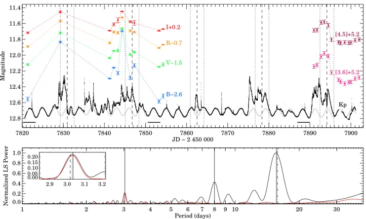
The top panel of Fig.2displays the short cadence light curve of DQ Tau. With vertical dashed lines we over- plotted the periastron times using the orbital elements fromCzekala et al.(2016). The dotted lines indicate the uncertainty by propagating the errors in the epoch of periastron and the orbital period. The 80-day-long K2 light curve covers 5 orbital cycles. As expected, there are brightening events of 0.2–0.4 mag coinciding with each periastron, with various durations and light curve mor- phologies. There was one cycle when a similar brightening event could be observed around the apastron. For the remaining time, the variability is dominated by a sinusoidal pattern with slightly varying phase and amplitude, and brief flare-like brightenings.

We calculated the Lomb-Scargle periodogram of the K2 light curve, which is plotted with a black curve in the bottom panel of Fig. 2. The normalized periodograms of the short and long cadence data gave identical results. The three most significant periods, all with False Alarm Probability below 10⁻⁸, are 15.627 ± 1.075 d, 8.003 ± 0.262 d, and 3.033 ± 0.044 d. The first one is consistent within the uncertainties with the orbital period of 15.80158±0.00066 d of the spectroscopic binary (Czekala et al. 2016), as expected because of the brightenings around the periastrons. The second one is half of the first period, and is a consequence of brightenings both at periastron and (sometimes) at apastron as well. The third and shortest period is consistent with the rotational period of the stars reported previously by Basri et al. (1997), indicating the presence of starspots on either or both stars leading to rotational modulation in the light curve.

4.2. Sinusoidal variations in the light curve We found an approximately 3 d periodicity in the K2 light curve. Remarkably, using vsini of 10 km s⁻¹, stellar radius of 1.6R⊙, and inclination of 23^◦ from Mathieu et al. (1997), the derived rotational period is also 3 d. We note, however, that while more recent radial velocity studies give similarvsini values (Nguyen et al.

2012 gave 14.7 and 11.3 km s⁻¹ for the primary and secondary, respectively, while Czekala et al. 2016 gave 14 and 11 km s⁻¹), the smaller stellar radii (1.05 and 1.00 R⊙ calculated from the stellar luminosity and temperature by Tofflemire et al. 2017) mean that these numbers would give much shorter rotational periods, on

the order of 1.4–1.7 d. Nevertheless, the K2 light curve clearly suggests that either both stars have a rotational period of about 3 d, or (if not both stars are spotted) the spotted component has a rotational period of 3 d.

In order to be able to precisely study the rotational modulation in the K2 light curve, we needed to dis- card the periastron-related brightenings and any other irregular flux variations. For this purpose, we phase- folded our K2 light curve with the 15.80158 d orbital period, and found that the periastron-related activity is mostly confined to phases between 0.75–1.1 (the periastron being at phase 0), in accordance with the findings of Tofflemire et al. (2017). We discarded these points, as well as those brighter than 12.65 mag. We recalcu- lated the periodogram for the remaining data points, which is plotted with a red curve in the bottom panel of Fig.2. The new periodogram has the strongest peak at the stellar rotational period, but with a small shift compared to the full data set: 3.027 ± 0.041 d. We phase-folded the light curve with this period, and found that the folded curve can be very well fitted with a sine curve. However, the data points showed a large scatter around the fitted sine curve, not explained by the photometric uncertainty, which is on the order of 10⁻⁴mag.

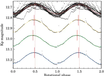
Motivated by this, we fitted sine functions separately to each rotational cycle, in order to look for systematic phase shifts or amplitude changes. Indeed, we found a gradual phase change from the first cycle to the last, which suggested that the period determined from the periodogram is still slightly biased. We determined the period which resulted in no systematic phase shifts (although some phase difference between the individual cycles still remained), and obtained P=3.017±0.004 d.

Fig. 3 shows the K2 light curve folded with this period and the fitted sine function, which has an average magnitude and peak-to-peak amplitude of<Kp>= 12.7189±0.0001 mag and ∆Kp= 0.0905±0.0001 mag, respectively.

4.3. Flare detection and characteristics

As previously described, we determined the exact phase, amplitude, and magnitude shift of each 3.017 d cycle. Interpolating linearly between these numbers, we calculated the phase, amplitude, and magnitude shift for each point in time during the K2 observations, and constructed a sinusoidal wave with a continuously changing phase, amplitude, and magnitude shift. This wave is plotted in Fig. 2 with a thick gray curve. Then we subtracted this sinusoidal wave from the original light curve, thereby creating a data set where the rotational modulation is corrected for. We used the resulting light curve, plotted in Fig.4, to look for short (typically a few

(6)

7820 7840 7860 7880 7900 JD − 2 450 000

12.8 12.6 12.4 12.2 12.0 11.8 11.6 11.4

Magnitude

7830 7850 7870 7890

I+0.2 R−0.7

V−1.5

B−2.6

[4.5]+5.2

[3.6]+5.2

Kp

1 10

Period (days) 0.0

0.2 0.4 0.6 0.8 1.0

Normalized LS Power

2 3 4 5 6 7 8 9 20 30

2.9 3.0 3.1 3.2

0.000.05 0.10 0.15 0.20

Figure 2. Top: short cadence K2 light curve of DQ Tau (small black dots), along with ground-basedBV(RI)C (blue, green, yellow and red dots) andSpitzer 3.6 and 4.5µm photometry (pink and purple dots). For clarity, the light curves were shifted along the y axis by the values indicated in the graph. Vertical dashed lines mark the periastron times using the orbital elements fromCzekala et al.(2016). The dotted lines indicate the uncertainty by propagating the errors in the epoch of periastron and the orbital period. The thick horizonal lines mark those three cycles that are plotted in Fig.3. The thick gray sinusoidal curve indicates the rotationally modulated periodic component of the light curve. Bottom: Lomb–Scargle periodogram of the K2 light curve (with black for the full data set, with red with the dataset where the brightenings close to periastron were discarded).

Solid vertical lines indicate the three most significant periods, while the dash-dotted line marks the spectroscopic binary’s orbital period. The small inset shows a zoom-in around the rotational period. The solid line marksP=3.033 d, the peak found for the full data set, the dotted line marks P=3.027, the peak found for the data set without the periastron brightenings, while the dashed line marksP=3.017 d, the period needed to get no systematic phase shifts during the 80-day-long K2 monitoring.

hours long) flare-like brightening events. We searched for flares by visually inspecting the light curve and its second derivative. We looked for events similar to a single classical flare (see, e.g., Gershberg 1972), which ideally consists of a fast rise phase and an exponential decay phase, as described by Hawley et al.(2014) and Davenport et al.(2014), or complex flares consisting of multiple eruptions. We identified 40 such events, with the caveat that we might have missed some very faint flares that were difficult to discern from the noise. These are highlighted with red color in Fig.4.

For each flare, we fitted a second or third order poly- nomial baseline to the points preceding and following the flare, and subtracted it. The resulting flare light curves (normalized to their peak values for better comparison) are plotted in Figs. 12 and 13. In order to establish whether these flares are similar to the classical flares typ-

ical in M-type stars, we fitted our data points with the flare template constructed by Davenport et al. (2014), see their Fig. 4 and Eqn. 1 and 4. We fitted the flare templates using the Levenberg-Marquardt least-squares minimization procedure coded inIDL(Interactive Data Language) byMarkwardt(2009). By looking at the fitted flare templates plotted in red over our Figs.12and 13, it is evident that many of the observed flares are well fitted by the template, but there are a few exceptions. In some cases, the rise phase is well fitted, while the decay phase is not exactly: the beginning of the decay phase follows the template shape, but then there is often an excess first and a deficiency later (e.g., flares #6 and #12).

In other cases, especially visible for the strongest flares, the beginning of the decay phase is steeper, while later it becomes shallower than the template (e.g., flares #1,

#21, or #40). This suggests that the double exponential

(7)

0.0 0.5 1.0 1.5 2.0 Rotational phase

13.2 13.1 13.0 12.9 12.8 12.7

Kp magnitude

Figure 3. Phase-folded long cadence K2 light curve of DQ Tau using P=3.017 d, together with a sine function fitted for the full data set (red dashed curve). The data points and sine fits below display three single cycles, between JD−2 450 000 = 7820.23–7823.26, 7850.56–7853.59, and 7886.95–7889.99. For clarity, these have been shifted along the y axis. The corresponding time intervals are marked in Fig. 2 with thick horizontal lines. The sine fits to the single cycles (dashed yellow, green, and blue curves) clearly show that they give slightly different phases, but with this period, there is no systematic phase change over the 80 days of observations. To guide the eye, the vertical red lines mark the maxima of the sine functions.

with the particular exponents Davenport et al. (2014) used is not always a good representative of DQ Tau’s flares. In some cases, the flares had distinct triangular shapes (e.g., flare #7), which are very different from the classical flare template and cannot be well fitted with it. In some cases, we could fit the light curves with the sum of several flare templates, indicating that DQ Tau displayed some complex flares. Out of the 40 flares, 25 were single classical flares, while 15 were complex flares.

4.4. Periastron brightenings

In order to construct a light curve which is devoid not only of rotational modulation but also of flares, as a next step we subtracted the flare templates fitted in the previous subsection from the light curve. The remaining variability mostly consists of complex brightening events clustered around the periastrons. It is very un- likely that these events are stellar flares, because they last for several days (even the shorter brightening at JD−2 450 000 = 7862.4 lasted for about 20 hours), while typical flares are shorter than a few hours. The light curve morphology is also distinctly different from the short brightening and exponential fading expected for flares. We tried to fit the periastron events with the sum of multiple flare templates, but we could not obtain

adequate fits. Another argument againts the periastron brightenings being due to complex flares is the different color. Our multi-filter optical monitoring covered two periastron events (Fig.2). While the brightening amplitudes decrease from theBtoIband (∆R= 0.44×∆B, thus the object becomes bluer when brighter, the observed colors are still redder than those of typical stellar flares (∆R= 0.17×∆B,Davenport et al. 2012). Based on these arguments, in agreement withTofflemire et al.

(2017), we can conclude that the variability remaining after removing the rotational modulation and the stellar flares are most probably due to variable accretion onto the stars.

Tofflemire et al. (2017) used theirU-band light curve as a proxy for the mass accretion rate. They first calculated theU-band excess luminosity above the stellar photosphere, then used a correlation betweenLUexcess and L^acc from Gullbring et al. (1998) to estimate the total accretion luminosity:

log(L^acc/L⊙) = 1.09 log(LUexcess/L⊙) + 0.98, from which the accretion rate can be calculated as follows:

M˙ = LaccR∗

GM∗

1− R∗

Rⁱⁿ

−1 .

In order to construct the best possible time-resolution monitoring of the accretion rate in the DQ Tau system, we attempted to use the K2 light curve as a proxy for the accretion. First we confirmed that the colors of the periastron events according to our multi-filter observations and according toTofflemire et al.(2017)’s data are consistent in the common filters (BV R). Then we plotted the variability amplitudes measured byTofflemire et al.

(2017) as a function of wavelength using the effective wavelengths of theU BV R filters. Then, using 740 nm as the effective wavelength of the K2 observations for DQ Tau, we extrapolated how much larger the variability is in theU band compared to K2. We found that the U-band variability is 6.4 times that of the K2-band in magnitude scale. Using this information, we could convert our K2 light curve (after subtracting the sinusoidal variation and flares) to aU-band light curve, then calculated the accretion rate using the same formulae and stellar parameters asTofflemire et al.(2017). Following their example, we also calculated the total accreted material in each orbital cycle (from phase 0.7 to phase 1.3).

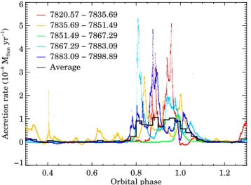
Our results can be seen in Fig.5.

As it was already evident from the light curve in Fig.2, the accretion rate curve in Fig. 5 confirms that the brightenings caused by the increased accretion rate are happening preferentially near periastron. The phase- folded accretion rate curve and its average in Fig. 6

(8)

7820 7840 7860 7880 7900 JD − 2 450 000

0.2 0.0

−0.2

−0.4

−0.6

Magnitude difference

7830 7850 7870 7890

Figure 4. K2 light curve of DQ Tau after removing the sinusoidal variation due to rotational modulation. Points highlighted with red color indicate the identified flares (Section4.3), while the blue points mark possible “dipper” events (Section5.5). As in Fig.2, dashed lines mark the periastrons and dotted lines indicate their uncertainties.

7820 7840 7860 7880 7900

JD − 2 450 000

−1 0 1 2 3 4 5 6

Accretion rate (10−8 MSun yr−1 )

7830 7850 7870 7890

0.0 0.2 0.4 0.6 0.8 1.0 1.2 1.4

Accreted mass per cycle (10−10 MSun)

Figure 5. Accretion rate as a function of time (black curve) and mass accreted per orbital cycle (large black dots connected by gray lines) in the DQ Tau system. As in Fig.2, dashed lines mark the periastrons and dotted lines indicate their uncertainties.

shows that significant accretion mostly happens between phases 0.75 and 1.1, as already noted byTofflemire et al.

(2017). The strongest peaks reach 5×10⁻⁸M⊙yr⁻¹, when the accretion luminosity goes up to 0.8L⊙. We observed increased accretion at each periastron covered by the K2 monitoring. The total mass accreted in each orbital cycle is typically about 1.2×10⁻¹⁰M⊙, except for a rather weak event at JD−2 450 000 = 7862.4. The un- precedented precision and high cadence of the K2 observations reveal fine details in the accretion rate changes, like a typical three-peaked shape, which is evident not only in some individual events but also in their average plotted by a black histogram in Fig.6. We note that, to our best knowledge, such an accretion rate curve shape is not predicted by any numerical simulations of accretion in a binary system. While two peaks could be explained by a time difference in the maximal accretion onto the two stars, we have no explanation for three peaks.

A more detailed inspection of the periastron events hints at another periodic phenomenon in the accretion rate. For example, in the last monitored periastron

event, the accretion rate displays several narrow maxima which seem to follow each other at multiples of 8.8 h (Fig. 5). Similar phenomenon although with different period might be present at the other periastron events as well. This suggests that the accretion process is not smooth, but the star probably accretes clumpy material.

5. DISCUSSION 5.1. Spots on the stars

We phase-folded Tofflemire et al. (2017)’s data with the orbital period ofCzekala et al.(2016) and discarded data points between phases 0.75–1.1, and also discarded points brighter than U=15.05 mag, B=14.65 mag, V=13.50 mag, and RC=12.35 mag, to exclude possible flares and apastron accretion events. Then we phase-folded the remaining points with a P=3.017 d, the rotational period obtained from the K2 light curve.

The result, which can be seen in Fig. 7 is sinusoidal, at least inBV RC, because theU-band data is so noisy (or contaminated by flares) that it might as well be consistent with constant brightness. We fitted a sine

(9)

0.4 0.6 0.8 1.0 1.2 Orbital phase

−1 0 1 2 3 4 5 6

Accretion rate (10−8 MSun yr−1 )

7820.57 − 7835.69 7835.69 − 7851.49 7851.49 − 7867.29 7867.29 − 7883.09 7883.09 − 7898.89 Average

Figure 6. Accretion rate in the DQ Tau system, phase- folded with the orbital period of 15.80158 d. Different colors mark the five consecutive cycles that K2 covered. The corresponding JD−2 450 000 values are displayed in the upper left corner. The black histogram shows the average accretion rate along the orbit in 0.025 wide phase bins. Phase 1.0 corresponds to the periastron.

curve to each of the B,V andRC light curves keeping the amplitude, magnitude offset, and phase as free parameters. The three light curves gave the same phase.

As expected for stellar spots, the variability amplitude we obtained is smaller towards longer wavelengths, with peak-to-peak values of ∆B = 0.20 mag, ∆V = 0.20 mag,

∆R= 0.17 mag.

As a next step, we tried to fitTofflemire et al.(2017)’s data with the analytic spot model of Budding (1977).

We estimated the intensity ratio between the quiet photosphere and the active regions by blackbody models with appropriate temperatures. The linear limb dark- ening coefficients were taken from Claret et al. (2012).

A good fit could be achieved using a model contain- ing three circular spots with homogeneous temperature.

The stability of such models is discussed in details in K˝ov´ari & Bartus(1997). By modeling the color indices, we found that the temperature of the cool spots are

≈400 K colder than the stellar surface, for which we took 3600 K (the average effective temperature of the two components of the binary). The three spots are located at longitudes of 230^◦, 350^◦, and 360^◦(with an uncertainty of±5^◦), at latitudes of 4^◦, 25^◦, and 90^◦. These parameters were fixed during the fitting, as there is only very limited information encoded about these in the photometric data. The angular radii of the spots are 43^◦, 41^◦, and 8^◦ (with an uncertainty of±5^◦), meaning that the three spots together cover about 50% of the star.

A polar spot is generally used to account for the uncertainty in the unspotted brightness (the model is sensitive

0.0 0.5 1.0 1.5 2.0

Rotational phase 15.5

15.0 14.5 14.0 13.5 13.0 12.5

Magnitude

R V−0.5

B−1.0

U−0.5

Figure 7.Top: phase-folded ground-based optical photometry of DQ Tau based on data fromTofflemire et al. (2017) and usingP=3.017 d, together with the brightness predicted by our fitted spot model (black curves). For clarity, the magnitudes in the different filters were shifted along the y axis by the values indicated in the graph. The typical error bar for each filter is displayed in the right-hand side. Bottom: a schematic representation of the spot distribution.

to even very small changes of this parameter) and long- term brightness variations, while the other two spots fit the exact quasi-sinusoidal light curve shape. The syn- thetic light curves produced by our spot model is over- plotted in Fig.7. The bottom of the figure also shows a schematic depiction of the spot coverage. Our model has peak-to-peak variability amplitudes of ∆B = 0.26 mag,

∆V = 0.22 mag, ∆R= 0.18 mag.

Our multi-filterBV(RI)C monitoring of DQ Tau obtained during the K2 campaign provided only 10 epochs, out of which 7 were taken close to periastron. Only three are left to characterize the color of the quiescent sinusoidal light variations. These data, within the uncertainty, are consistent with the quiescent color variations measured byTofflemire et al.(2017). However, the 3.017 d period component of the K2 light curve displayed smaller variability amplitude and a different phase. This suggests that during the K2 monitoring, the DQ Tau system had a different spot coverage than before, during Tofflemire et al. (2017)’s monitoring. The similar colors indicate that the temperature of the spots did not, while the different phase and amplitude indicate

(10)

that the location and extent of the spots did change during the 2.5 years that elapsed between their observations and our K2 study. We obtained a phase shift of 0.73 compared to Tofflemire et al. (2017)’s data, which corresponds to a difference of about 97^◦(roughly a quar- ter rotation). We could obtain a reasonably good fit by keeping the three spots in our model at the same latitute as before, but shift their longitude and decrease their radius to account for the smaller variability amplitude (a likely result of surface evolution that can be also observed in the quiet K2 data). On average, the spots covered about 30% of the stellar photosphere during the K2 observations. Moreover, we also discovered that the spot coverage can change on a significantly shorter timescale as well, as proven by the variable phases of the sine functions during the 80 days of the K2 monitoring (Fig.3).

It is an interesting question whether the spots are located on the primary, on the secondary, or both stars are spotted. Our photometric observations give no clue about this, and in our spot modeling, we assumed only one star. In practice, considering that the two stars are almost identical, having one star with about 50% spot coverage and another one with 0%, or having two stars with 25%-25% spot coverage would give the same light curves. Therefore, the obtained results should be used with caution. Detailed spectroscopic studies may reveal fine details in the photospheric line profiles of each star, which may help to decide the spot coverage of the individual components in the future.

5.2. Flares in the DQ Tau system

By converting the K2 counts to power in erg s⁻¹ as described in Section 3, and integrating the flare light curves over time, we calculated the energy released in each flare. We obtained values between 4.4×10³²erg and 1.2×10³⁵erg. The cumulative distribution of flare energies is displayed in Fig.8. Flares are often described by a power-law trend of the energy–cumulative flare frequency distribution (Gershberg 1972). If the number of flares (dN) in a given energy range (E+dE) is expressed as

dN(E)∝E^−αdE,

the cumulative flare distribution should have a slope of β = 1−α in log-log scale (see alsoHawley et al. 2014 andGizis et al. 2017). For DQ Tau, Fig.8indicates that apart from the lowest energies (where completeness is not secure) and the highest energies (which suffer from low number statistics), the cumulative distribution can be fitted with a power law with an exponent of β =

−0.51, from whichα= 1.51. An alternative method to determineαis to use the maximum likelihood estimator

(Arnold 2014):

(α−1) =n

" n

X

i=1

ln Ei

Emin

#⁻¹ ,

wherenis the number of flares detected, andEmin and Ei are the lowest and individual flare energies, respectively. For small samples the result is biased, which can be corrected by multiplying by a factor of ⁿ⁻²_n . This yields α = 1.40, which suggests that the flares are of non-thermal origin (cf. Aschwanden et al. 2016), and which places DQ Tau close to the very active M3–M5 sample ofHawley et al.(2014).

We also measured the duration of the flares as the time interval where the points are higher than the 1σnoise of the adjacent portions of the light curves. The flares we found have durations between 0.6 and 5.8 hours, with almost two thirds of the flares being 100–200 minutes long. The cumulative distribution of the flare durations is quite steep, its power law exponent is−3.02 (Fig.8).

By calculating for each flare the phase where they occurred, we checked whether there is any rotational or orbital phase when flares can preferentially be seen or are particularly energetic. We found, however, that the corresponding (lower) panels of Fig. 8 display a seemingly random distribution. To quantitatively decide whether the flares really occur at random phases, we run one-sided Kolmogorov-Smirnov and Kuiper tests to assess whether the phases are drawn from a uniform distribution. The obtained probabilities were 0.90 and 0.81 for the orbital phases and 0.98 and 0.92 for the rotational phases, using the two different test, respectively. This result means that the distribution of flares is not significantly different from a random distribution.

By applying Wilcoxon rank test to compare the phase sample with a randomly generated uniform distribution we came to the same conclusion. In order to examine whether the energy of flares has any influence on the phase distribution we divided the phases into two subsamples of equal size that contain the 20 brightest and 20 faintest flares. Using two-sided Kolmogorov-Smirnov and Kuiper tests, as well as the Wilcoxon rank test, we found no statistically significant difference between the two subsamples.

Concerning the orbital phases, this suggests that the flares are probably not related to magnetospheric in- teractions, because their occurrence is equally proba- ble when the binary components are far away from or close to each other, suggesting that they are more likely single-star flares. Accepting the single-star scenario, the flares could be happening in active regions above stellar spots, as seen on the Sun. This could indicate a connection between the photospheric and chromospheric

(11)

32.5 33.0 33.5 34.0 34.5 35.0 log(Energy/erg)

0.01 0.10 1.00

Cumulative flare distribution

−0.51

1.4 1.6 1.8 2.0 2.2 2.4 2.6

log(Duration/min) 0.01

0.10 1.00

Cumulative flare distribution

−3.02

0.0 0.5 1.0 1.5 2.0

Rotational phase 32

33 34 35 36

log(Energy/erg)

0.0 0.5 1.0 1.5 2.0

0 1 2 3 4 5 6 7

Number of flares

0.0 0.5 1.0 1.5 2.0

Orbital phase 32

33 34 35 36

log(Energy/erg)

0.0 0.5 1.0 1.5 2.0

0 1 2 3 4 5 6 7

Number of flares

Figure 8. Flare characteristics in DQ Tau.

activity, as reported for V374 Peg (Vida et al. 2016).

In other stars, this connection is mainly shown as an anticorrelation of the Hα line intensity and the light curve intensity (e.g., EY Dra,Korhonen et al. 2010, on the T Tauri-type star TWA 6, Skelly et al. 2008, but also on RS CVn-type binaries like RT Lac,Frasca et al.

2002). However, this connection is not always present:

on SAO 51891 no such relation was found (Biazzo et al.

2009). If such a connection holds for DQ Tau, one would expect to observe more flares around rotational phase 0, which corresponds to the faintest state of the system, i.e., when the most spotted (and therefore most active) side of the star faces us. While this is exactly what was observed in LkCa 4 and LkCa 7 by Vrba et al. (1993), such effect is not evident from our data on DQ Tau. A possible reason for this is that such a large fraction of the stellar surface is covered by spots that flares can be observed practically at any time.

Because our K2 photometry is unresolved, there is no way to discern whether the flares originated from the primary or the secondary. Since the binary is composed of two almost identical stars, we can expect similar flare activity from them both, and it would be reasonable to assume that about half of the detected flares come from each individual star. To account for this, we randomly removed half of the flares and repeated our analyses described above. We found that our main results do not change, therefore our main conclusions still hold.

We noted that for some flares (typically the brighter, single flares), the flare template does not fit the light curves well. The residual light curve from a fit to the peak and the first 5 minutes after the peak shows a slow brightening followed by a long decrease of intensity. This excess emission is unlike a typical flare sig- nature, therefore it must have a different origin, such as heating of one star due to the energy released by a flare or coronal mass ejections (CMEs) on the other star. We calculated the actual distance of the two stars during flares #1, #21, and #40 (0.07, 0.23 and 0.11 au, respectively), and the velocity needed to travel these distances, and obtained values between≈30 000−100 000 km s⁻¹for five minute post-peak travel time. These values would vary only slightly if we assume large magnetic loops of ≈1 R∗. The typical velocity of solar CMEs is on the order of a few hundred km s⁻¹, and the fastest detected stellar CME (on the late-type main sequence star AD Leo) had a maximum projected velocity of

≈5800 km s⁻¹(Houdebine et al. 1990). These are an order of magnitude smaller than the speed needed for the ejecta to reach the other component in the DQ Tau system, which makes the CME scenario less likely. Direct heating by illumination, however, is still possible.

5.3. Pulsed accretion in the DQ Tau system The accretion process from a circumbinary disk to the binary components has been extensively studied in the literature by means of numerical simulations. Although many of these works focus on (super)massive black hole

(12)

binary systems, some results are independent of the applied distance or mass scales. For unequal-mass, eccentric binaries, a common result of these models is that the accretion happens in short bursts and displays a clear periodicity at the binary’s orbital period (Cuadra et al.

2009; Roedig et al. 2011; Sesana et al. 2012). This is triggered by the secondary, which gravitationally per- turbs the inner edge of the circumbinary disk during each apoapsis passage and pulls some material from the disk that eventually lands on the binary components.

Therefore, it is not surprising that the secondary, which is closer to the disk and has a greater specific angular momentum, accretes more mass (Cuadra et al. 2009).

In some models, half and third of the orbital period can also be seen in the periodogram of the accretion rate.

These are related to the second and third frequency har- monics and are more pronounced for higher eccentrici- ties (Roedig et al. 2011). Although DQ Tau is closer to equal-mass than what was used in these simulations (M¹/M² = 0.33−0.35), the orbital period and its half appear in its periodogram.

In magnetohydrodynamic simulations of an equal- mass circular binary,Shi et al.(2012) found a gap radius (inner radius of the circumbinary disk) of twice that of the binary separation and bursts in the accretion rate at a period of about twice the binary’s orbital period.

Hydrodynamic simulations by (Mu˜noz & Lai 2016) indicated that equal-mass circular binaries display a quasi- periodic accretion rate curve with a dominant period of 5 times the binary’s orbital period. This corresponds to the orbital period of the innermost region of the circumbinary disk. On the other hand, the accretion rate in eccentric binaries shows larger variability with pulses in the accretion at a period equal to the binary’s orbital period. Indeed, in the almost equal-mass eccentric DQ Tau system, we see large variability in the accretion rate and a period close to the orbital period. Interest- ingly, the gap radius in DQ Tau is smaller and there the Keplerian period coincides with the orbital period (Sec. 5.4).

D’Orazio et al.(2013) made an extensive study of the accretion rate in black hole binaries with different mass ratios. They also found that the size of the inner gap is at most twice that of the binary separation (for equal- mass binaries) and decreases for more extreme mass ratios. An important result they obtained was that for binaries between q=0.25–1 mass ratio, the accretion rate showed three distinct periods, at 0.5, 1, and 5.7 times the binary’s orbital period. They claim that the last one is related to a dense lump of material that formed in the inner disk created by shocks due to a stream of material starting from the inner disk, and therefore depends

on the disk properties. However, the two periods with 1:2 ratio is a robust prediction of their model, which is independent of the disk properties, and could serve as an evidence for the presence of a binary. Interestingly, the two most significant periods in DQ Tau have a ratio of 0.51±0.06, suggesting that the model predictions of D’Orazio et al.(2013) for binary black holes may actually work for young stellar binaries as well. This raises the possibility that if the accretion-related variability in a young star’s light curve displays two significant periods with a 1:2 ratio, this may serve as a strong hint for binarity. Farris et al.(2014) went a step further and claimed that the periodicities observed in the accretion rate may even be used to infer the mass ratio of the binary.

G¨unther & Kley (2002) modeled several circumbinary disks surrounding classical T Tau stars, including DQ Tau. They found a flow of material from the inner edge of the circumbinary disk onto the central stars and that the accretion rate depends on the orbital phase.

They could match both the accretion rate and the spectral energy distribution of the model to the observed properties of the DQ Tau system. They found minimal accretion rates of a few times 10⁻⁹M⊙yr⁻¹, and peak accretion rates between 1–2×10⁻⁸M⊙yr⁻¹. Accord- ing to their simulations, the accretion rate both to the primary and to the secondary peaked exactly at periastron. This is actually in contrast to what we observe in DQ Tau, where there are typically several peaks per orbit and they all occur before the periastron, between phases of 0.8–1.0, see Fig.6. The measured peak accretion rate values agree well with the simulations. Another difference between our accretion rate curve and that of G¨unther & Kley(2002, see their Fig. 12) for DQ Tau is that the simulated accretion rate changes continuously, while in our observations the accretion pulses are often separated by long quiescent periods when the accretion rate is practically constant zero. This suggests a less continuous mass flow and a lower average mass accretion rate than what is obtained in the model.

5.4. Disk variability in the DQ Tau system OurSpitzer3.6µm and 4.5µm measurements are dis- tributed over a 11.4-day-long interval, which is 70% of an orbital period. The observations cover almost en- tirely the last periastron event that occurred during the K2 monitoring, except the very steep initial flux rise.

There are also mid-infrared data points from the quiescent part following the optical peak, and they cover the epoch of the apastron, too.

The measured emission at the Spitzerwavelengths is a combination of the stellar photosphere, modulated by

(13)

12.8 12.6 12.4 12.2 12.0 11.8 11.6

Magnitude

Kp [3.6]+5.3 [4.5]+5.3

7888 7890 7892 7894 7896 7898 7900 7902 JD − 2 450 000

800 850 900 950

T (K)

Figure 9. Top: K2 andSpitzerlight curves of DQ Tau after the removal of rotational modulation. Bottom: temperature variations in the inner disk of DQ Tau based on blackbody fits to theSpitzerdata.

the rotating stellar spots, and the disk’s thermal emission. None of ourSpitzerepochs coincided with a stellar flare, thus, any possible contribution from flares can be neglected in our case. In order to determine the disk emission, first we subtracted from the measured mid- infrared light curves a constant photospheric contribution (0.187 Jy and 0.098 Jy at 3.6µm and 4.5µm, respectively, based on our SED fitting explained in Section3).

Then we used the spot model presented in Section 5.1, and calculated how the sinusoidal curve seen in the Ke- pler light curve would appear at theSpitzerwavelengths using blackbody curves for the stellar photosphere and for the spots as well. This periodic signal was also subtracted from the Spitzer light curve, thus the residual flux and its variability reflects the thermal emission of the disk’s dust particles only.

The cleaned Spitzer light curve closely follows the Kepler optical magnitude changes also cleaned from the photosphere, the spots and the flare contributions (Fig.9). They both outline a large periastron peak that lasts for about 5 days and hint for a small local maximum at the very end of the K2 light curve, also confirmed by the Spitzer data. This correlated behavior strongly suggests that the variability in the disk’s thermal emission is caused by the changing optical brightness of the central stellar system.

In order to check for any possible time delay between the optical and infrared data sets, which may provide information about the irradiation process of the disk by the central stars, we performed a cross-correlation analysis by interpolating the Kepler curve at theSpitzer epochs, shifting theSpitzerlight curve by different time lags and calculating χ² values between the two data sets after transforming them to a common flux scale via a linear transformation. Surprisingly, we obtained two equally deep minima in the χ² distribution. One

constitutes a small delay of ∆t= 1.44 h, the other corresponds to a shift of 10.32 h. In both cases theSpitzer light curve lagged behind the optical one. Considering the relatively coarse sampling of theSpitzerdata set, the first minimum is consistent with no delay. The second minimum with 10.32−1.44 = 8.88 h lag behind the first one may not stem from a real phyical process, but may correspond to the average time difference between neigh- boring localized narrow maxima during the periastron event (Section4.4). The result that no significant delay was observed between the optical and the infrared light curves suggests that the variable component of the the mid-IR emission primarily originates from the optically thin surface layer of the disk, where the temperature of the dust particles can adapt to a variable radiation field within seconds (cf.Chiang & Goldreich 1997).

The shapes and fluxes of theSpitzerlight curves carry information on the disk geometry. An estimate of the disk inner radius can be derived from theSpitzer data.

At each epoch, we fitted the 3.6µm and 4.5µm fluxes (after subtracting the photosphere and the spot components) by a single temperature blackbody curve, assuming that the mid-infrared radiation is emitted from the disk’s inner edge. With a physically motivated prescrip- tion that the main changes are related to the variable temperature while the emitting area remains constant, we fixed the latter parameter at an average value, and reproduced the Spitzer fluxes by varying the temperature only. The obtained temperatures are plotted in the bottom panel of Fig.9. We found the highest temperature during the periastron event (917 K), while the temperatures in the quiescent interval were as low as 825 K.

Assuming equilibrium between the impinging radiation field and the thermal dust emission in quiescence, we can estimate the radius of the emitting region using the following equation:

L∗

4πR² =σT⁴.

From Tofflemire et al.(2017) we adopted L∗ = (0.19 + 0.13)L⊙= 0.32L⊙ for the binary’s luminosity (for simplicity assuming that both stars are located at the center), and obtained that the radius where the disk temperature is 825 K isR = 0.13 au. We can consider this radius as the inner edge of the (dust) disk (Fig.10). In- terestingly, this value is equal to the binary’s semimajor axis, while dynamical models of circumbinary disks predict a cleared inner hole with a radius of 1.8–2.6 times larger that the semimajor axis (Artymowicz & Lubow 1994). Another interesting fact is that the Keplerian orbital period at 0.13 au is 15.56 d, essentially identical to the orbital period of the binary (and of course to the period of the periastron brightenings). We can interpret

(14)

−0.3 −0.2 −0.1 0.0 0.1 0.2 0.3 Distance (au)

−0.2

−0.1 0.0 0.1 0.2

Distance (au)

Figure 10. Sketch of the DQ Tau system. The + sign marks the center of mass. The black ellipses indicate the two stars’ orbits using the orbital parameters and inclination fromCzekala et al.(2016). The parts of the orbit when elevated accretion typically happens (between phases 0.75–

1.1) are highlighted with thick black curves. The orange dots reflect the actual sizes of the stars using a stellar radius of 1.6R⊙, while the dotted orange circles highlight the size of the magnetosphere for a typical T Tauri star (5×R∗, Hartmann et al. 1994). The orange ring around the system indicates the inner part of the circumbinary disk, using 0.13 au as its inner radius, see Sec.5.4for details.

this result as the inner disk being in corotation with the orbit of the binary.

The absolute flux of the disk’s thermal emission is determined by the emitting area. Assuming that this area forms a ring whose inner radius isRⁱⁿ=0.13 au, we can calculate the outer radius as well. If the emitting area is optically thick, and the disk’s inclination is 22^◦ (Czekala et al. 2016), almost pole-on, then the outer radius of the emitting ring isR^out= 1.24×Rⁱⁿ= 0.16 au.

We note that we adopted a uniform temperature for this ring, but an outward decreasing radial temperature pro- file would not change the conclusions significantly.

The ratio of the disk’s luminosity (approximated by the integrated flux of the 825 K blackbody curve in quiescence) and the stellar luminosity of 0.32L⊙ is 0.163.

We can interpret this number as the solid angle of the inner disk as seen from the center of the system (neglect- ing again the orbital motion of the stars). This means that the height of the inner disk above the midplane is about 0.15×Rin, putting a constraint on the disk geometry.

While we computed a blackbody temperature of 825 K for the quiescent period from theSpitzerdata, the temperature during the peak of periastron event was higher, reaching 917 K. If the emitting area was the same as in quiescence, then the irradiating central luminosity had to increase proportionally to T⁴. This calculation

shows that the luminosity of the DQ Tau system had to increase from quiescence to the periastron peak by (917/825)⁴ = 1.53, reaching 0.49L⊙. Thus, the system emitted an excess luminosity of (0.49−0.32)L⊙= 6.5×10³²erg s⁻¹, which is close to the luminosity peak measured in theKeplerband during the last periastron event (taking into account the emission outside theKe- pler filter may bring the two numbers even closer to each other). This result supports our scenario that the increasing mid-infrared flux during the periastron event was due to increased irradiation of the inner edge of the circumbinary disk at about 0.13−0.16 au.

Finally we checked whether the free-fall time of the accreting material is consistent with the computed inner disk radius. Again placing both stars at the center for simplicity, we computed a free-fall time of 2.7 d from a distance of 0.13 au. This value is only half of the time difference between apastron (when the stars are clos- est to the disk’s inner edge and the perturbation of the disk is expected) and the periastron (when the brightness peak implies the infall of the material on the stellar surface). Considering the complicated path the material may take from the inner edge of the disk to the binary components, it is not at all unreasonable to assume that this would take as much time as that elapsed between apastron and periastron.

5.5. Dipper phenomenon in DQ Tau

Our results presented so far demonstrated the com- plexity of the accretion process, as well as the circumstellar and magnetic structure in the DQ Tau binary system. After removing the spot-related variability from the K2 light curve (Fig.4), apart from the flares and periastron events, another interesting phenomenon can be seen: dips in the light curve when the system seems to be fainter that what is expected from the stellar photosphere (also taking into account the spots). These dips are marked by blue color in Fig.4. They are typically 0.3–1.6 d long, and their depth is between 0.04–0.09 mag.

They seem to be happening at around rotational phase of 0.5, suggesting a possible connection with the stellar rotation, although they are not strictly periodic. A similar relationship was observed by Bodman et al.(2017) using K2 data on young stars in Upper Sco andρOph.

We found no obvious correlation with the orbital period.

The dipper phenomenon is explained as obscuration/eclipse by dusty clumps of material close to the inner edge of the disk. Bodman et al.(2017) presented a unified paradigm of the dipper phenomenon, and explained it by accretion streams that lift material out of the disk midplane at the magnetospheric truncation radius. This model also works for objects which are not