arXiv:1912.04839v4 [astro-ph.SR] 29 Apr 2020

(1)

arXiv:1912.04839v4 [astro-ph.SR] 29 Apr 2020

Preprint typeset using L^ATEX style emulateapj v. 12/16/11

HOMOGENEOUS ANALYSIS OF GLOBULAR CLUSTERS FROM THE APOGEE SURVEY WITH THE BACCHUS CODE. II. THE SOUTHERN CLUSTERS AND OVERVIEW

Szabolcs Mészáros^1,2,3, Thomas Masseron^4,5, D. A. Garc´ıa-Hernández^4,5, Carlos Allende Prieto^4,5, Timothy C. Beers⁶, Dmitry Bizyaev⁷, Drew Chojnowski⁸, Roger E. Cohen⁹, Katia Cunha^10,11, Flavia Dell’Agli^4,5, Garrett Ebelke¹², José G. Fernández-Trincado^13,14, Peter Frinchaboy¹⁵, Doug Geisler^16,17,18, Sten Hasselquist^19,20, Fred Hearty²¹, Jon Holtzman²², Jennifer Johnson²³, Richard R. Lane²⁴, Ivan Lacerna^13,25, Penelopé Longa-Peña²⁶, Steven R. Majewski¹², Sarah L. Martell²⁷,

Dante Minniti^28,29,30, David Nataf³¹, David L. Nidever^32,35, Kaike Pan⁷, Ricardo P. Schiavon³³, Matthew Shetrone³⁴, Verne V. Smith³⁵, Jennifer S. Sobeck¹¹, Guy S. Stringfellow³⁶, L´aszl´o Szigeti^1,3,

Baitian Tang³⁷, John C. Wilson¹², Olga Zamora^4,5 Draft version April 30, 2020

ABSTRACT

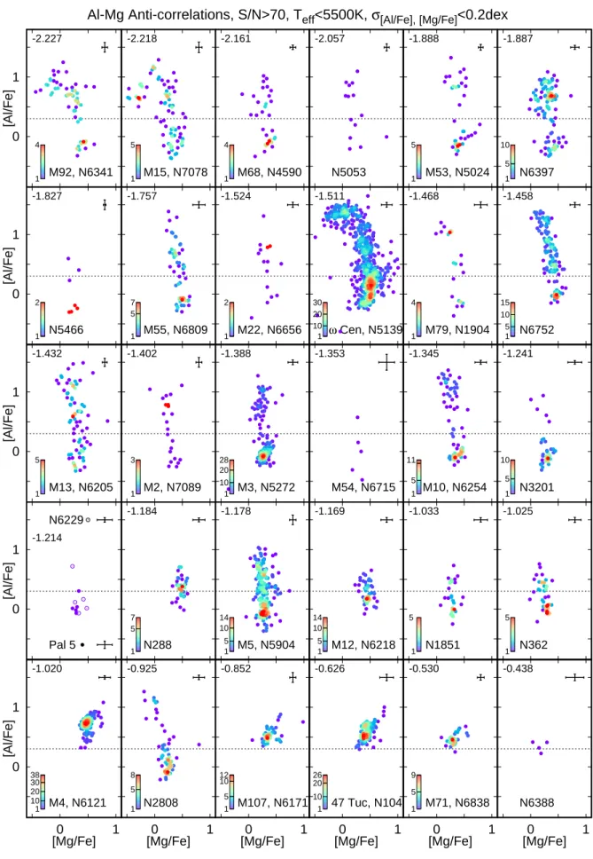
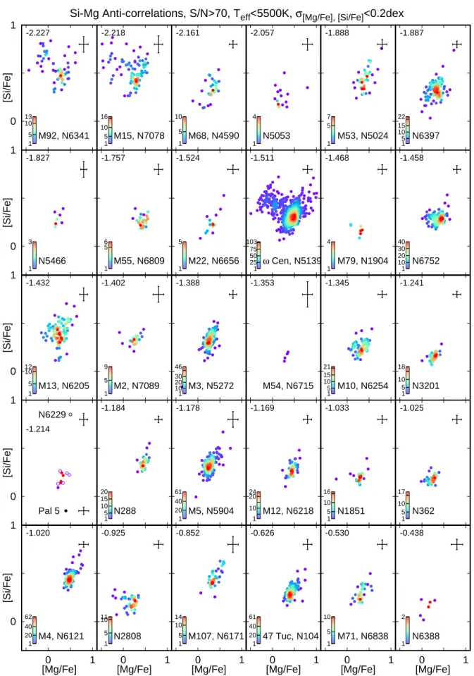
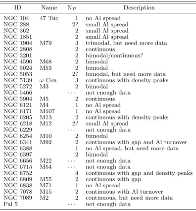
We investigate the Fe, C, N, O, Mg, Al, Si, K, Ca, Ce and Nd abundances of 2283 red giant stars in 31 globular clusters from high-resolution spectra observed in both the northern and southern hemisphere by the SDSS-IV APOGEE-2 survey. This unprecedented homogeneous dataset, largest to date, allows us to discuss the intrinsic Fe spread, the shape and statistics of Al-Mg and N-C anticorrelations as a function of cluster mass, luminosity, age and metallicity for all 31 clusters. We find that the Fe spread does not depend on these parameters within our uncertainties including cluster metallicity, contradicting earlier observations. We do not confirm the metallicity variations previously observed in M22 and NGC 1851. Some clusters show a bimodal Al distribution, while others exhibit a continuous distribution as has been previously reported in the literature. We confirm more than 2 populations in ωCen and NGC 6752, and find new ones in M79. We discuss the scatter of Al by implementing a correction to the standard chemical evolution of Al in the Milky Way. After correction, its dependence on cluster mass is increased suggesting that the extent of Al enrichment as a function of mass was suppressed before the correction. We observe a turnover in the Mg-Al anticorrelation at very low Mg in ω Cen, similar to the pattern previously reported in M15 and M92. ω Cen may also have a weak K-Mg anticorrelation, and if confirmed, it would be only the third cluster known to show such a pattern.

1. INTRODUCTION

1ELTE Eötvös Loránd University, Gothard Astrophysical Ob- servatory, 9700 Szombathely, Szent Imre H. st. 112, Hungary

2Premium Postdoctoral Fellow of the Hungarian Academy of Sciences (meszi@gothard.hu)

3MTA-ELTE Exoplanet Research Group, 9700 Szombathely, Szent Imre h. st. 112, Hungary

4Instituto de Astrof´ısica de Canarias (IAC), E-38205 La La- guna, Tenerife, Spain

5Universidad de La Laguna (ULL), Departamento de As- trof´ısica, 38206 La Laguna, Tenerife, Spain

6Dept. of Physics and JINA Center for the Evolution of the Elements, University of Notre Dame, Notre Dame, IN 46556, USA7Apache Point Observatory, P.O. Box 59, Sunspot, NM 88349

8Dept. of Astronomy, New Mexico State University, Las Cruces, NM 88003, USA

9Space Telescope Science Institute, 3700 San Martin Drive, Baltimore, MD 21218, USA

10Steward Observatory, University of Arizona, 933 North Cherry Avenue, Tucson, AZ 85721, USA

11Observatório Nacional, São Cristóvão, Rio de Janeiro, Brazil

12Dept. of Astronomy, University of Virginia, Charlottesville, VA 22904-4325, USA

13Instituto de Astronom´ıa y Ciencias Planetarias, Universi- dad de Atacama, Copayapu 485, Copiap´o, Chile

14Institut Utinam, CNRS-UMR 6213, Université Bourgogne- Franche-Compté, OSU THETA Franche-Compté, Observatoire de Besan¸con, BP 1615, 251010 Besan¸con Cedex, France

15Department of Physics & Astronomy, Texas Christian Uni- versity, Fort Worth, TX 76129, USA

16Departamento de Astronom´ıa, Universidad de Concepci´on, Casilla 160-C, Concepci´on, Chile

During most of the 20th century it was believed that globular clusters (GCs) exhibit only one generation of stars. However, detailed photometric and spectroscopic studies of Galactic globular clusters over the past thirty years have revealed great complexity in the elemental abundances of their stars, from the main sequence through to the asymptotic giant branch. Most light elements show star-to-star variations in almost all GCs and these large variations are generally interpreted as the result of chemical feedback from an earlier generation of stars (Gratton et al. 2001; Cohen et al. 2002), rather than inhomogeneities in the original stellar cloud from which these stars formed. Thus, the current scenario of GC evolution generally assumes that more than one population of stars were formed in each cluster, and the chemical makeup of stars that formed later is polluted by material produced by the first generation.

The origin of the polluting material remains to be es- tablished and it has obvious bearings on the timescales for the formation of the cluster itself and its mass bud- get. Proposed candidate polluters include intermediate mass stars in their asymptotic giant branch (AGB) phase (Ventura et al. 2001), fast rotating massive stars losing mass during their main sequence phase (Decressin et al.

2007), novae (Maccarone & Zurek 2012), massive bi- naries (de Mink et al. 2009), and supermassive stars (Denissenkov et al. 2014). These potential contributions obviously operate on different time scales and require a different amount of stellar mass in the first generation.

(2)

In order to constrain these models and to gain an overall understanding of the multiple stellar populations in globular clusters we need comprehensive studies with a relatively complete and unbiased data set. This requires a focused effort by Galactic archaeology surveys to ob- tain and uniformly analyze spectra for large samples of globular cluster stars across a wide range of metallicity.

There are two main fronts in exploring multiple populations (MPs) in GCs: photometry and spectroscopy.

Several larger photometric surveys have been conducted to explore MPs in almost all GCs (e.g., Piotto et al. 2007;

Sarajedini et al. 2007; Piotto et al. 2015; Milone et al.

2017; Soto et al. 2017), using the data from the Hub- ble Space Telescope achieving unprecedented photometric precision. Using high-resolution spectroscopy the Lick-Texas group (e.g., Sneden et al. 2004, 2000, 1992, 1991, 1997; Kraft et al. 1992, 1995; Ivans et al. 2001) conducted the first large survey of northern clusters using three different telescopes and spectrographs. Also using high-resolution spectroscopy Carretta et al. (2009a,b,c) have carried out the first detailed survey of southern clusters with the VLT telescopes, exploring the Na-O and Al-Mg anticorrelations, which are the result of Ne- Na and Mg-Al cycles occurring in the H-burning shell of the first population stars whose nucleosynthetic prod-

17Instituto de Investigacin Multidisciplinario en Ciencia y Tec- nolog´ıa, Universidad de La Serena. Avenida Ral Bitrn S/N, La Serena, Chile

18Departamento de Astronom´ıa, Facultad de Ciencias, Univer- sidad de La Serena. Av. Juan Cisternas 1200, La Serena, Chile

19Dept. of Physics & Astronomy, University of Utah, Salt Lake City, UT, 84112, USA

20NSF Astronomy and Astrophysics Postdoctoral Fellow

21 Dept. of Astronomy and Astrophysics, The Pennsylvania State University, University Park, PA 16802, USA

22New Mexico State University, Las Cruces, NM 88003, USA

23Dept. of Astronomy, The Ohio State University, 140 W. 18th Ave., Columbus, OH 43210, USA

24 Instituto de Astro´ısica, Pontificia Universidad Catalica de Chile, Av. Vicuna Mackenna 4860, 782-0436 Macul, Santiago, Chile

25Instituto Milenio de Astrof´ısica, Av. Vicu˜na Mackenna 4860, Macul, Santiago, Chile

26Centro de Astronomia, Universidad de Antofagasta, Avenida Angamos 601, Antofagasta 1270300, Chile

27School of Physics, University of New South Wales, NSW 2052, Australia

28Departamento de Ciencias Fisicas, Facultad de Ciencias Ex- actas, Universidad Andres Bello, Av. Fernandez Concha 700, Las Condes, Santiago, Chile

29Millennium Institute of Astrophysics, Av. Vicuna Mackenna 4860, 782-0436, Santiago, Chile

30Vatican Observatory, V00120 Vatican City State, Italy

31Dept. of Physics and Astronomy, Johns Hopkins University, Baltimore, MD, 21218, USA

32Dept. of Physics, Montana State University, P.O. Box 173840, Bozeman, MT 59717-3840, USA ; National Optical Astronomy Ob- servatory, 950 North Cherry Avenue, Tucson, AZ 85719, USA

33Astrophysics Research Institute, IC2, Liverpool Science Park, Liverpool John Moores University, 146 Brownlow Hill, Liverpool, L3 5RF, UK

34University of Texas at Austin, McDonald Observatory, Fort Davis, TX 79734, USA

35National Optical Astronomy Observatory, Tucson, AZ 85719, USA

36Center for Astrophysics and Space Astronomy, Dept. of As- trophysical and Planetary Sciences, University of Colorado, 389 UCB, Boulder, CO 80309-0389, USA

37 School of Physics and Astronomy, Sun Yat-sen University, Zhuhai, China

ucts were later distributed through the cluster. We refer the reader to Bastian & Lardo (2018) for a complete overview on MPs in GCs.

With the appearance of high spectral resolution sky surveys some of these southern clusters were revisited by the Gaia-ESO survey (Gilmore et al. 2012) focusing on the same two element pairs (Pancino et al. 2017). The first homogeneous exploration of 10 northern clusters was carried out by M´esz´aros et al. (2015), which was updated by Masseron et al. (2019), both using data from the SDSS-III (Eisenstein et al. 2011) Apache Point Observa- tory Galactic Evolution Experiment (APOGEE) survey.

Results for additional clusters observed by APOGEE were published by Schiavon et al. (2017), Tang et al.

(2017), and Fern´andez-Trincado et al. (2019). Its successor, SDSS-IV (Blanton et al. 2017) APOGEE-2 (Majewski et al. 2017) started in the summer of 2014 and ends in 2020, further expanding the number of observed GCs from the southern hemisphere. Compari- son of northern and southern clusters was difficult previously because many observations were carried out with different telescopes and abundance determination tech- niques that may have systematic errors of their own.

The APOGEE survey is the first spectroscopic survey that covers both the northern and southern sky by in- stalling two twin spectrographs, identical in design, on the Sloan 2.5 meter telescope (Gunn et al. 2006) at the Apache Point Observatory (APO) and the du Pont 2.5m telescope at Las Campanas Observatory (LCO). In an effort to create the first truly systematic study of the chemical makeup of multiple populations in all GCs, Masseron et al. (2019) reanalyzed the 10 clusters observed from APO (M´esz´aros et al. 2015) with an updated pipeline.

In this paper we discuss 21 new (mostly southern) clusters observed from both LCO and APO by following the same steps of atmospheric parameter and abundance determination as Masseron et al. (2019) and com- bine them with the 10 northern clusters discussed by Masseron et al. (2019). Because M12 was observed from both observatories, we use this cluster to check how homogeneous the abundances are from APO and LCO. By combining observations from APO and LCO, we are able to discuss the statistics of Al-Mg and N-C anticorrelations as a function of main cluster parameters in a much larger sample of clusters than was previously possible.

Na-O anticorrelation is not included in our study, because Na lines in the H-band are too weak to be observ- able in almost all of our sample of clusters.

There are various labels used in the literature for stars within GCs that are enriched in He, N, Na, Al and are depleted in O, C and Mg, such as second generation stars and chemically enriched stars. We will use the term second generation/population (SG) stars when referring to stars that have [Al/Fe]>0.3 dex, and first generation/population (FG) when [Al/Fe]<0.3 dex (see Section 5.1). While more than two populations can be identified based on abundances in some clusters, we focus on simplifying the term to refer to all stars that satisfy the above criteria, as second/first generation/population stars for easier discussion. On the other hand most metal-rich clusters ([Fe/H]>−1) are enriched in Al ([Al/Fe]>0.3 dex), but appear to host only a single population of stars, so they are chemically enriched but

(3)

Table 1

Properties of Clusters from the Literature

ID Name N1a N2b [Fe/H] E(B−V) Rt Vdisp RA Dec Vhelio µα∗ µδ

All S/N>70 ´ km/s km/s mas yr⁻¹ mas yr⁻¹

NGC 104 47 Tuc 186 151 -0.72 0.04 42.9 12.2 00 24 05.67 -72 04 52.6 -17.2 5.25 -2.53

NGC 288 43 40 -1.32 0.03 12.9 3.3 00 52 45.24 -26 34 57.4 -44.8 4.22 -5.65

NGC 362 56 40 -1.26 0.05 16.1 8.8 01 03 14.26 -70 50 55.6 223.5 6.71 -2.51

NGC 1851 43 30 -1.18 0.02 11.7 10.2 05 14 06.76 -40 02 47.6 320.2 2.12 -0.63

NGC 1904 M79 26 25 -1.60 0.01 8.3 6.5 05 24 11.09 -24 31 29.0 205.6 2.47 -1.59

NGC 2808 77 71 -1.14 0.22 15.6 14.4 09 12 03.10 -64 51 48.6 103.7 1.02 0.28

NGC 3201 179 152 -1.59 0.24 28.5 5.0 10 17 36.82 -46 24 44.9 494.3 8.35 -2.00

NGC 4147 3 1 -1.80 0.02 6.3 3.1 12 10 06.30 +18 32 33.5 179.1 -1.71 -2.10

NGC 4590 M68 37 36 -2.23 0.05 13.7 3.7 12 39 27.98 -26 44 38.6 -93.2 -2.75 1.78

NGC 5024 M53 41 39 -2.10 0.02 30.3 5.9 13 12 55.25 +18 10 05.4 -63.1 -0.11 -1.35

NGC 5053 17 17 -2.27 0.01 11.8 1.6 13 16 27.09 +17 42 00.9 42.5 -0.37 -1.26

NGC 5139 ωCen 898 775 -1.53 0.12 57.0 17.6 13 26 47.24 -47 28 46.5 232.7 -3.24 -6.73

NGC 5272 M3 153 148 -1.50 0.01 38.2 8.1 13 42 11.62 +28 22 38.2 -147.2 -0.14 -2.64

NGC 5466 15 7 -1.98 0.00 34.2 1.6 14 05 27.29 +28 32 04.0 106.9 -5.41 -0.79

NGC 5634 2 0 -1.88 0.05 8.4 5.3 14 29 37.30 -05 58 35.0 -16.2 -1.67 -1.55

NGC 5904 M5 207 191 -1.29 0.03 28.4 7.7 15 18 33.22 +02 04 51.7 53.8 4.06 -9.89

NGC 6121 M4 158 153 -1.16 0.35 32.5 4.6 16 23 35.22 -26 31 32.7 71.0 -12.48 -18.99

NGC 6171 M107 66 55 -1.02 0.33 17.4 4.3 16 32 31.86 -13 03 13.6 -34.7 -1.93 -5.98

NGC 6205 M13 127 103 -1.53 0.02 25.2 9.2 16 41 41.24 +36 27 35.5 -244.4 -3.18 -2.56

NGC 6218 M12 86 54 -1.37 0.19 17.6 4.5 16 47 14.18 -01 56 54.7 -41.2 -0.15 -6.77

NGC 6229 7 5 -1.47 0.01 10.0 7.1 16 46 58.79 +47 31 39.9 -138.3 -1.19 -0.46

NGC 6254 M10 87 84 -1.56 0.28 21.5 6.2 16 57 09.05 -04 06 01.1 74.0 -4.72 -6.54

NGC 6316 1 1 -0.45 0.54 5.9 9.0 17 16 37.30 -28 08 24.4 99.1 -4.97 -4.61

NGC 6341 M92 70 67 -2.31 0.02 15.2 8.0 17 17 07.39 +43 08 09.4 -120.7 -4.93 -0.57

NGC 6388 26 9 -0.55 0.37 6.2 18.2 17 36 17.23 -44 44 07.8 83.4 -1.33 -2.68

NGC 6397 158 141 -2.02 0.18 15.8 5.2 17 40 42.09 -53 40 27.6 18.4 3.30 -17.60

NGC 6441 17 5 -0.46 0.47 8.0 18.8 17 50 13.06 -37 03 05.2 17.1 -2.51 -5.32

NGC 6522 7 5 -1.34 0.48 16.4 8.2 18 03 34.02 -30 02 02.3 -14.0 2.62 -6.40

NGC 6528 2 1 -0.11 0.54 16.6 6.4 18 04 49.64 -30 03 22.6 211.0 -2.17 -5.52

NGC 6539 1 1 -0.63 1.02 21.5 5.9 18 04 49.68 -07 35 09.1 35.6 -6.82 -3.48

NGC 6544 7 7 -1.40 0.76 2.05 6.4 18 07 20.58 -24 59 50.4 -36.4 -2.34 -18.66

NGC 6553 8 7 -0.18 0.63 8.2 8.5 18 09 17.60 -25 54 31.3 0.5 0.30 -0.41

NGC 6656 M22 80 20 -1.70 0.34 29.0 8.4 18 36 23.94 -23 54 17.1 -147.8 9.82 -5.54

NGC 6715 M54 22 7 -1.49 0.15 10.0 16.2 18 55 03.33 -30 28 47.5 142.3 -2.73 -1.38

NGC 6752 153 138 -1.54 0.04 55.3 8.3 19 10 52.11 -59 59 04.4 -26.2 -3.17 -4.01

NGC 6760 3 3 -0.40 0.77 7.2 · · · 19 11 12.01 +01 01 49.7 -1.6 -1.11 -3.59

NGC 6809 M55 96 92 -1.94 0.08 16.3 4.8 19 39 59.71 -30 57 53.1 174.8 -3.41 -9.27

NGC 6838 M71 39 35 -0.78 0.25 9.0 3.3 19 53 46.49 +18 46 45.1 -22.5 -3.41 -2.61

NGC 7078 M15 133 104 -2.37 0.10 21.5 12.9 21 29 58.33 +12 10 01.2 -106.5 -0.63 -3.80

NGC 7089 M2 26 24 -1.65 0.06 21.5 10.6 21 33 27.02 -00 49 23.7 -3.6 3.51 -2.16

Pal 5 5 5 -1.41 0.03 16.3 0.6 15 16 05.25 -00 06 41.8 -58.4 -2.77 -2.67

Pal 6 5 4 -0.91 1.46 8.4 · · · 17 43 42.20 -26 13 21.0 181.0 -9.17 -5.26

Terzan 5 7 7 -0.23 2.28 13.3 19.0 17 48 04.80 -24 46 45.0 -82.3 -1.71 -4.64

Terzan 12 1 1 -0.50 2.06 · · · · · · 18 12 15.80 -22 44 31.0 94.1 -6.07 -2.63

Note. — Average metallicities, reddenings, tidal radii and coordinates were taken from Harris 1996 (2010 edition). Radial and dispersion velocities are from Baumgardt & Hilker (2018). Proper motions were taken from Baumgardt et al. (2019).

a The number of all stars in our sample.

bThe number of stars with S/N>70.

Table 2

Atmospheric Parameters and Abundances of Individual Stars

2MASS ID Cluster Status T_eff log g [Fe/H] σ_[Fe/H] [C/Fe] limit^a σ_[C/Fe] NC [N/Fe] ...

2M13121714+1814178 M53 RGB 4574 0.87 -2.007 0.121 · · · 0 · · · 0 · · ·

2M13122857+1815051 M53 RGB 4202 -0.07 -1.982 0.088 · · · 0 · · · 0 0.834

2M13123506+1814286 M53 RGB 4639 1.02 -1.894 0.124 · · · 0 · · · 0 · · ·

2M13123617+1807320 M53 RGB 4514 0.74 -1.841 0.083 · · · 0 · · · 0 · · ·

2M13123617+1827323 M53 RGB 4652 1.05 -1.928 0.119 · · · 0 · · · 0 · · ·

Note. — This table is available in its entirety in machine-readable form in the online journal. A portion is shown here, with reduced number of columns, for guidance regarding its form and content. Star identification from Carretta et al. (2009b) was added in the last column.

a The number of lines used in the abundances analysis from BACCHUS (Masseron et al. 2016).

(4)

Table 3

Abundance Averages and Scatter

ID Name [Fe/H] [Fe/H] Mass V_ABS Age [Fe/H] [Fe/H] [Fe/H]^a [Al/Fe] [Al/Fe]

Carretta Pancino 10³ M⊙ Average Scatter Error Average Scatter

NGC 104 47 Tuc -0.768 -0.71 779 -9.42 12.8 -0.626 0.107 0.082 0.583 0.129

NGC 288 -1.305 · · · 116 -6.75 12.2 -1.184 0.114 0.059 0.368 0.175

NGC 362 · · · -1.12 345 -8.43 10.0 -1.025 0.080 0.056 0.241 0.240

NGC 1851 · · · -1.07 302 -8.33 · · · -1.033 0.082 0.077 0.192 0.251

NGC 1904 M79 -1.579 -1.51 169 -7.86 12.0 -1.468 0.092 0.062 0.449 0.530

NGC 2808 -1.151 -1.03 742 -9.39 11.2 -0.925 0.101 0.070 0.328 0.446

NGC 3201 -1.512 · · · 149 -7.45 11.1 -1.241 0.102 0.061 0.099 0.345

NGC 4590 M68 -2.265 · · · 123 -7.37 12.7 -2.161 0.100 0.108 0.302 0.419

NGC 5024 M53 · · · · · · 380 -8.71 12.7 -1.888 0.101 0.108 0.346 0.507

NGC 5053 · · · · · · 56.6 -6.76 12.3 -2.057 0.095 0.108 0.397 0.447

NGC 5139 ωCen · · · · · · 3550 -10.26 · · · -1.511 0.205 0.077 0.586 0.533

NGC 5272 M3 · · · · · · 394 -8.88 11.4 -1.388 0.127 0.068 0.249 0.425

NGC 5466 · · · · · · 45.6 -6.98 13.6 -1.827 0.070 0.105 0.246 0.663

NGC 5904 M5 -1.340 · · · 372 -8.81 11.5 -1.178 0.102 0.062 0.297 0.346

NGC 6121 M4 -1.168 · · · 96.9 -7.19 13.1 -1.020 0.086 0.042 0.708 0.121

NGC 6171 M107 -1.033 · · · 87 -7.12 13.4 -0.852 0.106 0.076 0.538 0.118

NGC 6205 M13 · · · · · · 453 -8.55 11.7 -1.432 0.129 0.078 0.536 0.517

NGC 6218 M12 -1.310 · · · 86.5 -7.31 13.4 -1.169 0.094 0.073 0.279 0.164

NGC 6229 · · · · · · 291 -8.06 · · · -1.214 0.127 0.038 0.189 0.276

NGC 6254 M10 -1.575 · · · 184 -7.48 12.4 -1.345 0.102 0.074 0.451 0.549

NGC 6341 M92 · · · · · · 268 -8.21 13.2 -2.227 0.096 0.133 0.562 0.414

NGC 6388 -0.441 · · · 1060 -9.41 11.7 -0.438 0.074 0.152 0.341 0.078

NGC 6397 -1.988 · · · 88.9 -6.64 13.4 -1.887 0.092 0.088 0.451 0.408

NGC 6656 M22 · · · · · · 416 -8.50 12.7 -1.524 0.112 0.092 0.461 0.407

NGC 6715 M54 · · · · · · 1410 -9.98 10.8 -1.353 0.039 0.059 0.189 0.499

NGC 6752 -1.555 -1.48 239 -7.73 13.8 -1.458 0.076 0.052 0.634 0.455

NGC 6809 M55 -1.934 · · · 188 -7.57 13.8 -1.757 0.080 0.067 0.358 0.454

NGC 6838 M71 -0.832 · · · 49.1 -5.61 12.7 -0.530 0.112 0.088 0.463 0.099

NGC 7078 M15 -2.320 · · · 453 -9.19 13.6 -2.218 0.121 0.136 0.438 0.446

NGC 7089 M2 · · · -1.47 582 -9.03 11.8 -1.402 0.069 0.055 0.400 0.464

Pal 5 · · · · · · 13.9 -5.17 · · · -1.214 0.085 0.073 0.053 0.130

[Al/Fe] [Al/Fe] [Al/Fe] f_enriched S1^b S1^b [N/Fe] [N/Fe] S2^c S2^c Average Average Scatter Average Scatter Average Scatter Average Scatter

>0.3dex <0.3dex >0.3dex

NGC 104 47 Tuc 0.586 · · · 0.128 · · · 0.393 0.074 0.924 0.407 0.486 0.112

NGC 288 0.462 0.175 0.121 · · · 0.418 0.054 0.832 0.341 0.487 0.107

NGC 362 0.468 0.049 0.125 · · · 0.214 0.050 1.038 0.360 0.306 0.112

NGC 1851 0.495 0.033 0.095 · · · 0.251 0.056 1.034 0.355 0.274 0.128

NGC 1904 M79 0.826 -0.136 0.288 0.609 0.248 0.029 · · · · · · · · · · · ·

NGC 2808 0.802 0.025 0.341 0.391 0.203 0.056 0.937 0.440 0.327 0.120

NGC 3201 0.635 -0.081 0.198 0.252 0.221 0.053 0.789 0.351 0.37 0.069

NGC 4590 M68 0.648 -0.111 0.207 0.545 0.323 0.093 · · · · · · · · · · · ·

NGC 5024 M53 0.917 -0.061 0.182 0.417 0.444 0.101 · · · · · · · · · · · ·

NGC 5053 0.772 -0.029 0.208 · · · 0.27 0.127 · · · · · · · · · · · ·

NGC 5139 ωCen 0.935 0.058 0.389 0.603 0.413 0.096 1.273 0.452 0.642 0.177

NGC 5272 M3 0.809 -0.027 0.203 0.331 0.303 0.083 0.861 0.297 0.373 0.187

NGC 5466 · · · -0.161 · · · · · · 0.258 0.058 · · · · · · · · · · · ·

NGC 5904 M5 0.604 0.010 0.196 0.484 0.307 0.078 1.094 0.393 0.359 0.154

NGC 6121 M4 0.709 · · · 0.121 · · · 0.489 0.064 0.894 0.269 0.376 0.086

NGC 6171 M107 0.538 · · · 0.118 · · · 0.429 0.087 0.911 0.468 0.6 0.123

NGC 6205 M13 0.860 -0.050 0.325 0.644 0.368 0.097 1.248 0.268 0.471 0.116

NGC 6218 M12 0.444 0.154 0.088 · · · 0.373 0.064 1.028 0.347 0.548 0.089

NGC 6229 · · · 0.057 · · · · · · 0.283 0.056 0.571 0.052 · · · · · ·

NGC 6254 M10 0.981 -0.039 0.265 0.481 0.317 0.066 1.136 0.291 0.512 0.096

NGC 6341 M92 0.770 -0.092 0.197 0.759 0.439 0.087 · · · · · · · · · · · ·

NGC 6388 0.381 · · · 0.045 · · · 0.158 0.088 1.020 0.323 0.341 0.098

NGC 6397 0.701 -0.094 0.177 0.686 0.338 0.092 · · · · · · · · · · · ·

NGC 6656 M22 0.662 -0.100 0.248 · · · 0.306 0.111 · · · · · · · · · · · ·

NGC 6715 M54 · · · -0.072 · · · · · · 0.243 0.025 · · · · · · · · · · · ·

NGC 6752 0.832 0.004 0.326 0.761 0.365 0.053 1.054 0.197 0.38 0.106

NGC 6809 M55 0.734 -0.066 0.249 0.531 0.378 0.051 1.093 0.102 · · · · · ·

NGC 6838 M71 0.477 · · · 0.088 · · · 0.318 0.080 0.992 0.441 0.661 0.113

NGC 7078 M15 0.752 -0.056 0.231 0.613 0.417 0.097 · · · · · · · · · · · ·

NGC 7089 M2 0.785 -0.061 0.212 0.545 0.313 0.048 1.058 0.132 0.413 0.154

Pal 5 · · · -0.009 · · · · · · 0.229 0.044 0.699 0.224 0.353 0.087

Note. — This table lists statistics for 31 GCs remaining after our refining procedure described in Section 2 and 3.1. Scatter is defined as the standard deviation around the mean. Masses are taken from Baumgardt & Hilker (2018), and we use the ages compiled by Krause et al.

(2016).

a The error of [Fe/H] is the average uncertainty for a given cluster.

b[(Mg+Al+SI)/Fe].

c[(C+N+O)/Fe].

(5)

any possible SG stars have the same [Al/Fe] content as FG stars within our errors (see Section 7.3 for more discussion). We treat these clusters as having one FG star group when looking at MPs based on Al abundances.

2. MEMBERSHIP ANALYSIS Observed Stars 12

13 14 15 16

0.5 1 1.5 M15N7078

V

12 13 14 15

16 0.5 1 1.5 M92 N6341

12 13 14 15

160.5 1 1.5 M68 N4590

14 15 16

0.5 1 1.5 M53 N5024

11 12 13 14 15

0.5 1 1.5 M55 N6809

V

11 12 13 14 15

0.5 1 1.5 2 47 Tuc N104

12 13 14 15 16

1 1.5 2 M12 N6218

12 13 14 15

1 1.5 2 M71N6838

11 12 13 14 15

0.5 1 1.5 2 N6752

V

12 13 14 15

16 1 1.5 2 M10 N6254

11 12 13 14 15

160.5 1 1.5 2 M4 N6121

11 12 13 14 15 16

0.5 1 1.5 2 N3201

13 14 15

16 1 1.5 2 N2808

V

12 13 14 15

160.5 1 1.5 2 N288

12 13 14 15 16

0.5 1 1.5 M3 N5272

13 14 15

1 1.5 2

M79N1904

11 12 13 14 15

0.5 1 1.5 2 M22N6656

V

11 12 13 14 15

160.5 1 1.5 2 ω Cen N5139

13 14 15

1 1.5 M2 N7089 B-V

12 13 14 15 16

0 0.5 1 1.5 2 M5N5904

12 B-V 13 14 15

160.5 1 1.5 2 M13 N6205

V

B-V 13 14 15

1 1.5 2 N1851

B-V

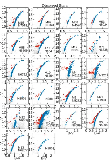
Figure 1. The CMD of observed stars by APOGEE in 22 clusters in common with Stetson et al. (2019). AGB/HB stars are denoted by red dots, the RGB stars are by blue dots.

Table 1 lists the globular clusters observed by APOGEE-2, along with the main parameters from the Harris catalog (Harris 1996 2010 edition), Gaia DR2 (Baumgardt et al. 2019) and from (Baumgardt & Hilker 2018). A more detailed description of the general target selection of APOGEE and APOGEE-2 can be found in Zasowski et al. (2013) and Zasowski et al. (2017), respectively. Our target selection follows that of M´esz´aros et al. (2015) and Masseron et al. (2019). We select stars based on their radial velocity first, their distance from cluster center second, and their metallicity third. In radial velocity, we required stars to be within three times the velocity dispersion of the mean cluster velocity, and in distance we required stars to be within the tidal radius. The metallicity cut was usually set to ±0.5 dex around the cluster average, except for clusters with suspected intrinsic Fe spread for which the metallicity cut was skipped, or only obvious field stars were deleted (for example stars with

solar-like metallicity in otherwise metal-poor clusters).

For this paper we made important updates by selecting the average cluster radial velocity and its scatter from Gaia DR2 (Baumgardt & Hilker 2018) rather than from Harris 1996 (2010 edition). In addition, we introduced a fourth step that is based upon selecting stars that have proper motion within a 1.5−2.5 mas yr⁻¹ range (depending on the cluster) around the cluster average proper motion from the Gaia DR2 catalog (Gaia Collaboration et al. 2018).

These two improvements were not adopted by Masseron et al. (2019), but now we refine the list of stars presented in that study. While the selected members of those 10 northern clusters have only changed slightly, because some stars were added or deleted, we did not re- derive atmospheric parameters and abundances for stars that remained members, as our analysis method has not changed. It is important to note that only a couple of stars have been deleted from these GCs, and the main science results and conclusions presented in Masseron et al.

(2019) remain the same. However, all figures, including data for those 10 clusters have been updated for this paper.

The individual atmospheric parameters and the derived abundances are listed in Table 2, while the abundance averages and RMS scatters for each cluster are presented in Table 3. Table 2 contains results for all stars and clusters that were analysed, altogether 3382 stars in 44 clusters. However, we do not discuss all clusters and stars. We make a quality selection according to the following criteria. High S/N spectra are essential to determine abundances from atomic and molecular features.

Most of the tests done by the APOGEE team concluded that abundances become reliable around S/N=70−100, however, objects with poorer S/N have also been an- alyzed and included in Table 2. The spectra have been processed by the APOGEE data processing pipeline (Nidever et al. 2015). Another criterion was that a cluster has to have at least 5 members with S/N>70 to qual- ify for further analysis. The following clusters did not meet this criterion: NGC 4147, NGC 5634, NGC 6316, NGC 6528, NGC 6539, NGC 6760, Pal 6 and Terzan 12.

While we do not use these clusters in our analysis, their abundances and atmospheric parameters were derived and listed in Table 2 for reference. The remaining 36 clusters were further refined based on their reddening values as described in the next section. Table 3 contains the clusters remaining after our refining procedure.

3. ATMOSPHERIC PARAMETERS AND ABUNDANCES 3.1. BACCHUS description

Since the method of deriving atmospheric parameters and abundances is identical to that of Masseron et al.

(2019), we only give a short overview of it in this paper.

We use the Brussels Automatic Code for Characterizing High accUracy Spectra (BACCHUS) (Masseron et al.

2016) to determine the metallicity and abundances, but not effective temperatures and surface gravities. Mi- croturbulent velocities were computed from the surface gravities using the following equation:

vmicro = 2.488−0.8665·logg+ 0.1567·log g·logg This relation was originally determined from the

(6)

Gaia-ESO survey by cancelling the trend of abundances against equivalent widths of selected Fe I lines (Masseron et al. 2019). The validity of this relation in the H-band was checked by (Masseron et al. 2019).

Due to problems with ASPCAP (Garc´ıa P´erez et al.

2014) effective temperatures at low metallicities, [M/H]< −0.7 dex (detailed by M´esz´aros et al.

2015; J¨onsson et al. 2018; Masseron et al. 2019;

Nataf et al. 2019; Nidever et al. 2019), these were computed from 2MASS colors using the equations from Gonz´alez Hern´andez & Bonifacio (2009). Surface gravities were derived from isochrones (Bertelli et al.

2008, 2009; Marigo et al. 2017) by taking into account their evolutionary state. The log g was determined by taking the photometric effective temperature and reading the log g, by interpolating through surface gravities, corresponding to that effective temperature from the isochrone. AGB and RGB stars were selected by combining our list of stars with the ground-based photometric catalog compiled by Stetson et al. (2019) for 22 clusters in common with our sample. Our selection was based on the star’s position on the V−(B−V) color- magnitude diagram (see e.g., Garc´ıa-Hern´andez et al.

2015) shown in Figure 1. For clusters not listed in the Stetson catalog we assumed all stars to be on the RGB.

For further information on our abundance determination methods, comparisons to ASPCAP, and their accuracy and precision (generally below 0.1 dex) we refer the reader to Section 3 of Masseron et al. (2019). The absorption lines selected for abundance determination are the same as used by Masseron et al. (2019). Random errors were derived from the line-by-line abundance dispersion.

The use of photometric temperatures introduces its own set of problems mostly related to high E(B−V) values. The Gonz´alez Hern´andez & Bonifacio (2009) relations are very sensitive to small changes in E(B−V), which is very important in high reddening clusters that may in addition suffer from significant differential reddening inside the cluster. For this reason the list of clusters was further limited by removing clusters with E(B−V)>0.4 according to the Harris catalog. Our metallicities derived from highly reddened spectra are also significantly larger than what the optical studies have found making us believe that either reddening and/or photometric temperatures are not reliable when E(B−V)>0.4. This issue is explored in more de- tail in Section 4.1. The following five clusters have at least 5 members with S/N>70, but have E(B−V)>0.4:

NGC 6441, NGC 6522, NGC 6544, NGC 6553 and Terzan 5. The final sample after the S/N and reddening cuts includes 2283 stars in 31 clusters, and we use this sample to study statistics of Mg-Al and N-C anticorrelations throughout the paper. Previous homogeneous surveys are listed in Table 4 for easy comparison.

While Table 2 lists all abundances we were able to measure regardless of S/N, we introduced the previously mentioned S/N>70 cut in all figures and statistics. Up- per limits are also listed in Table 2, but not plotted in any of the figures, or included when calculating cluster averages and scatters, because we made the decision to study the behavior of anticorrelations based on only real measurements. We implemented a maximum temperature cut of 4600 K for CNO and K, because for higher

temperatures the molecular (atomic in case of K) lines become too weak, rendering abundances of these elements unreliable. We use 5500 K for the rest of the elements as maximum temperature above which errors start to significantly increase. Stars plotted in all figures in Sections 4 to 8 have elemental abundances with internal errors smaller than 0.2 dex to reduce contamination from highly unreliable measurements. Stars with abundances outside these parameter regions are published in Table 2, but we caution the reader to carefully examine these values before drawing scientific conclusions. These limitations were set in place when calculating abundance averages and scatter for all clusters and are listed in Ta- ble 5. The error in the mean [Fe/H] is smaller than the dot used to represent the data in all figures, thus er- rorbars were not plotted in any of the figures. For the abundance−abundance plots we only highlighted the average error of each abundance for simplicity, but Table 2 lists all individual errors.

Comparisons of T_eff and logg with that of Carretta et al. (2009)

-600 -400 -200 0 200 400 600 800 1000

3500 4000

4500 5000

5500 6000

Teff - Teff, Carretta (K)

T_eff

-2 -1 0 1 2

0 1

2 3

4 log g - log gCarretta

log g

Figure 2. Top panel: Comparisons of our Teff scale from Gonz´alez Hern´andez & Bonifacio (2009) with Carretta et al.

(2009a,b,c), who used Alonso et al. (1999, 2001). Bottom panel:

Comparisons of our surface gravities with the same source.

3.2. Comparisons of Teff and log g Values with the Literature

We limit our discussion of comparisons of Teff and log g with literature to that of Carretta et al. (2009a,b,c),

(7)

Table 4

Overview of Homogeneous Spectroscopic Surveys of Globular Clusters

Reference Nstars Ncl Element Pairs^a Observatory^b Survey Comments Carretta et al. (2009a,b,c) 1958 19 Na-O, Al-Mg ESO/VLT Carretta UVES/Giraffe combined.

M´esz´aros et al. (2015) 428 10 Al-Mg, N-C APO APOGEE

Pancino et al. (2017) 572 9 Al-Mg ESO/VLT Gaia-ESO

Masseron et al. (2019) 885 10 Al-Mg, N-C APO APOGEE Same clusters as M´esz´aros et al. (2015).

Nataf et al. (2019) 1581 25 Al-Mg, N-C APO/LCO APOGEE Payne analysis only.

This paper 2283 31 Al-Mg, N-C APO/LCO APOGEE Includes data from Masseron et al. (2019).

Note. — Clusters with less than 5 observed members were excluded from the statistics.

aThe main element pairs used to study multiple populations.

bESO/VLT: Very Large Telescope at the European Southern Observatory, APO: Apache Point Observatory, LCO: Las Campanas Observatory.

Table 5

Selected Parameter Cuts for Analysis Abundance Teff [Fe/H] σ[X/Fe]

K dex dex

[C/Fe] <4600 >−1.9 <0.2 [N/Fe] <4600 >−1.9 <0.2 [O/Fe] <4600 >−1.9 <0.2 [Mg/Fe] <5500 >−2.5 <0.2 [Al/Fe] <5500 >−2.5 <0.2 [Si/Fe] <5500 >−2.5 <0.2 [K/Fe] <4600 >−1.5 <0.2 [Ca/Fe] <5500 >−2.5 <0.2 [Fe/H] <5500 >−2.5 <0.2 [Ce/Fe] <4400 >−1.8 <0.2 [Nd/Fe] <4400 >−1.8 <0.2 Note. — A S/N>70 cut is also applied. All averages and scatter values were computed using stars that satisfy these conditions including the figures shown in the paper.

since that is the literature source we have the most stars in common with, 514 altogether, out of the list of pa- pers in Table 4. Star identification from Carretta et al.

(2009b) was added to Table 2 for easy comparison.

The difference between our parameters and those of Carretta et al. (2009a,b,c) can be seen in Figure 2. The systematic offset seen between the two temperatures are the characteristics of the photometric temperature con- versions (and differences in colors used to calculate the temperature) of Gonz´alez Hern´andez & Bonifacio (2009) and Alonso et al. (1999, 2001), which was used by Carretta et al. (2009a,b,c). The temperature difference is generally between ±300 K, but it increases with in- creasing temperature.

Similar structure can be seen when comparing surface gravities, because the temperature and log g have a simple linear correlation on the RGB, so any systematic difference seen in the temperature scale will propagate to log g. These discrepancies may also propegate to metallicity, further discussed in Section 4.1, and/or individual abundances, which is expected when temperature scales differ from one another.

3.3. Comparisons of APO and LCO Observations As mentioned at the end of the introduction, APOGEE-2 uses two spectrographs identical in design at two observatories, APO and LCO to map all parts of the Milky Way. The identical design makes it possible to directly derive atmospheric parameters and abundances that are believed to be on the same scale by observing the

same stars from both observatories. The observing strat- egy is carefully planned (Zasowski et al. 2017) to observe stars with both telescopes that cover the full parameter range ASPCAP operates in so that any differences between the final results can be carefully studied and cali- brated if necessary. In terms of globular clusters, there is only one that has been observed with both the northern and southern telescopes: M12, which limits our comparisons to a small range in metallicity.

T_eff - [X/Fe] comparisons from APO and LCO in M12, S/N>70

-2 -1

∆[Fe/H] = 0.008

[Fe/H]

APO LCO

-1 0 1

∆[C/Fe] = -0.099

[C/Fe]

0 1

2 ∆[N/Fe] = 0.076

[N/Fe]

0 1

∆[O/Fe] = 0.036

[O/Fe]

0 1

4000 5000

∆[Mg/Fe] = 0.001

[Mg/Fe]

T_eff (K)

0

1 ∆[Al/Fe] = 0.028

[Al/Fe]

0

1 ∆[Si/Fe] = -0.013

[Si/Fe]

0

1 ∆[K/Fe] = 0.015

[K/Fe]

0 1

∆[Ca/Fe] = -0.013

[Ca/Fe]

0 1

4000 5000

∆[Ce/Fe] = -0.027

[Ce/Fe]

T_eff (K)

Figure 3. Comparison of stars observed from both APO (red dots) and LCO (black dots) in M12. The differences between APO and LCO printed in each panel are on the level or smaller than the average internal error of each element.

Figure 3 shows the BACCHUS derived abundances as

(8)

The BACCHUS Iron Scale Compared to Literature, E(B-V)<0.4, σ_[Fe/H]<0.2dex

-0.1 0 0.1 0.2 0.3 0.4

-2.5 -2 -1.5 -1 -0.5 0

No correction for different Solar references.

[Fe/H]BACCHUS - [Fe/H]Literature

[Fe/H]_BACCHUS

Harris catalog (2010 edition) Carretta et al. (2009)

Pancino et al. (2017) -0.1 0 0.1 0.2 0.3 0.4

-2.5 -2 -1.5 -1 -0.5 0

0.09 dex was subtracted from Carretta et al. (2009).

Average difference: 0.064dex

[Fe/H]BACCHUS - [Fe/H]Carretta

[Fe/H]_BACCHUS

0 0.1 0.2 0.3 E(B-V)

-0.1 0 0.1 0.2 0.3 0.4

-2.5 -2 -1.5 -1 -0.5 0

0.09 dex was subtracted from Carretta et al. (2009).

Average difference: -0.009dex

[Fe/H]Pancino - [Fe/H]Carretta

[Fe/H]_Pancino -0.1

0 0.1 0.2 0.3 0.4

-2.5 -2 -1.5 -1 -0.5 0

Average difference: 0.064dex Same solar reference.

[Fe/H]BACCHUS - [Fe/H]Pancino

[Fe/H]_BACCHUS

Figure 4. Comparison of mean [Fe/H] cluster values from various literature sources. Differences in the solar reference Fe abundances was corrected where indicated. The three different Fe scales agree roughly within±0.1 dex after correction.

a function of effective temperature of the 21 stars in M12 that were both observed from APO and LCO. The difference is calculated for each star that was observed with both telescopes and then averaged together over all the stars. The differences between the two sets of observations range between 0.001 dex for [Mg/Fe] to 0.099 dex for [C/Fe], all of which can be considered as a very good agreement. The discrepancy for C, N and O are generally larger than for the rest of elements, which is under- standable considering that it is more difficult to fit these molecular lines than simple unblended atomic absorption lines. All the differences are on par or smaller than the average error in M12, and thus we conclude that observations from APO and LCO can be directly compared to each other without worrying about any possible large systematic errors. While this test is limited to a unique metallicity ([Fe/H]=−1.2), similar tests on much lager samples of APO-LCO overlapping stars have been done on the ASPCAP-analysis of the DR16 data, suggesting that the data from APO and LCO indeed are of similar quality and yield very similar stellar parameters and abundances (J¨onsson et al. in prep.).

4. THE FE SCALE

The amount of iron observed in GCs allows the inves- tigation of the history of stars and intra-cluster medium from which the GCs have formed, because Fe is mostly the result of core-collapse supernovae of high and intermediate mass stars. Additionally, Fe is traditionally used as the tracer of metallicity - the overall abundance of metals in a star. Abundances of iron from homogeneous

high-resolution spectroscopic studies are also used to cal- ibrate low-resolution spectroscopic and photometric in- dices. Setting a true and absolute Fe scale is, thus, one of the most important goals of high-resolution abundance analysis.

4.1. Comparisons with Literature

We compare our metallicity scale with those of the Harris catalog, Carretta et al. (2009c) and Gaia-ESO (Pancino et al. 2017). The Harris catalog is a compila- tion of various literature sources and all our clusters were selected from it. The largest homogeneous study of iron abundances from high-resolution spectra was previously carried out by Carretta et al. (2009c), 17 of their clusters are in common with our sample, and we have 7 clusters that were also observed by Gaia-ESO. We show the four different iron scales on the top left panel of Figure 4. We find that the [Fe/H] metallicities we derive are on average 0.162 dex higher than those from the Harris catalog, 0.154 dex higher than Carretta et al. (2009c), 0.064 dex higher than Pancino et al. (2017).

These metallicity differences of GCs have been present in the APOGEE data since the very first data re- lease (M´esz´aros et al. 2013) and remained in place in all subsequent data releases (Holtzman et al. 2015, 2018;

Jönsson et al. 2018). This was verified by Mészáros et al.

(2015) and by Masseron et al. (2019) using the APOGEE line list, but effective temperatures and surface gravities independent of ASPCAP. Interestingly, Pancino et al.

(2017) have also found a similar, although slightly smaller, 0.08 dex higher metallicities than Carretta et al.