Article
Evaluation of the Terrestrial Ecosystem Model
Biome-BGCMuSo for Modelling Soil Organic Carbon under Different Land Uses
Maša Zorana Ostrogovi´c Sever1,*, Zoltán Barcza2,3,4 , Dóra Hidy3, AnikóKern5 , Doroteja Dimoski1, Slobodan Miko6 , Ozren Hasan6 , Branka Grahovac7and Hrvoje Marjanovi´c1
Citation: Ostrogovi´c Sever, M.Z.;
Barcza, Z.; Hidy, D.; Kern, A.;
Dimoski, D.; Miko, S.; Hasan, O.;
Grahovac, B.; Marjanovi´c, H.
Evaluation of the Terrestrial Ecosystem Model Biome-BGCMuSo for Modelling Soil Organic Carbon under Different Land Uses.Land2021, 10, 968. https://doi.org/10.3390/
land10090968
Academic Editors: Cezary Kabala and Manuel López-Vicente
Received: 28 July 2021 Accepted: 10 September 2021 Published: 14 September 2021
Publisher’s Note:MDPI stays neutral with regard to jurisdictional claims in published maps and institutional affil- iations.
Copyright: © 2021 by the authors.
Licensee MDPI, Basel, Switzerland.
This article is an open access article distributed under the terms and conditions of the Creative Commons Attribution (CC BY) license (https://
creativecommons.org/licenses/by/
4.0/).
1 Croatian Forest Research Institute, Cvjetno naselje 41, HR-10450 Jastrebarsko, Croatia;
doroteja@sumins.hr (D.D.); hrvojem@sumins.hr (H.M.)
2 Department of Meteorology, Eötvös Loránd University, Pázmány P. st. 1/A, H-1117 Budapest, Hungary;
zoltan.barcza@ttk.elte.hu
3 Excellence Center, Faculty of Science, Eötvös Loránd University, Brunszvik u. 2, H-2462 Martonvásár, Hungary; hidyd@elte.hu
4 Faculty of Forestry and Wood Sciences, Czech University of Life Sciences Prague, Kamýcká129, 16521 Prague, Czech Republic
5 Department of Geophysics and Space Sciences, Eötvös Loránd University, Pázmány P. st. 1/A, H-1117 Budapest, Hungary; anikoc@nimbus.elte.hu
6 Croatian Geological Survey, Sachsova 2, HR-10000 Zagreb, Croatia; smiko@hgi-cgs.hr (S.M.);
ohasan@hgi-cgs.hr (O.H.)
7 Ministry of Agriculture, Directorate for Professional Support to the Development of Agriculture and Fisheries, J. J. Strossmayera 3, HR-31500 Našice, Croatia; branka.grahovac@mps.hr
* Correspondence: masao@sumins.hr
Abstract:Soil organic carbon (SOC) is a mandatory pool in national inventory reports on greenhouse gas (GHG) emissions and removals to the UNFCCC. Hence, its accurate assessment is important.
Modelling SOC changes for national GHG reports is encouraged, but the uncertainty related to this pool still presents a significant challenge; thus, verifying modelling results with field observations is essential. We used the process-based model Biome-BGCMuSo and assessed its suitability for use in Croatia’s GHG reporting. We modelled SOC stocks in the top 30 cm of the mineral soil layer (SOC30) for four different land-use (LU) categories (Deciduous/Coniferous Forest, Grassland and Annual Cropland) distributed in three biogeographical regions (Alpine, Continental and Mediterranean) and compared them with results of a national soil survey. A total of 573 plot level simulations were undertaken and results were evaluated at three stratification levels (LU, LU×biogeographical region, and plot). The model reproduced the overall country mean of SOC30with no overall bias, and showed good performance at the LU level with no significant (p< 0.05) difference for all LUs except Deciduous Forest (11% overestimation). At finer stratifications, the model performance considerably worsened. Further model calibration, improvement and testing, as well as repeated soil survey are needed in order to assess the changes in SOC30and to evaluate the potential of the Biome-BGCMuSo model for use in GHG reporting.
Keywords:biogeochemical modelling; spatial modelling; soil national inventory; national inventory report; forests; croplands; grasslands
1. Introduction
Soil organic carbon (SOC) is one of five mandatory pools in national reports on greenhouse gas (GHG) emissions and removals that must be submitted pursuant to the United Nations Framework Convention on Climate Change (UNFCCC) and accounted for under the Kyoto Protocol (KP) [1] and Paris Agreement (PA) [2]. Carbon (C) emissions and removals within the SOC pool are included in the land use, land-use change and forestry (LULUCF) sector of the National Inventory Reports (NIR) of the Parties to the UNFCCC.
Land2021,10, 968. https://doi.org/10.3390/land10090968 https://www.mdpi.com/journal/land
LULUCF is the only sector that accounts for C removal; therefore, in some regions, it has been identified as essential in reaching the goal of climate neutrality (The European Green Deal) [3]. Considering that SOC is the largest terrestrial C pool [4,5] and that warmer climate can stimulate SOC losses [6,7], with the possibility of forming a positive feedback loop between the carbon cycle and climate warming [8], it is important to make an accurate assessment of SOC stocks and changes.
The uncertainties in the LULUCF sector estimates are currently being emphasised [9].
According to principles required by International Panel on Climate Change, national reports need to be transparent, complete, consistent, comparable and accurate [10]. This means that each party needs to deliver a fully documented report in which accurate estimates are given for all relevant categories (i.e., land uses and pools) of GHG sources and sinks, throughout the time series. Of all the mandatory pools, namely aboveground and belowground live biomass, deadwood, litter and soil organic matter, reporting on net C change in soil under different land uses (LU) over time is often most challenging.
The simplest approach of assessment (Tier 1) in mineral SOC stocks assumes no change, whereas the use of higher tiers requires integration of field measurements and modelling. Soil C modelling is cost effective and is already in use for national reporting where soil models such as RothC [11,12], Yasso07 [13–16] or CENTURY [17] have been used. Nevertheless, field measurements of soil C stocks, although expensive and time consuming, are necessary for model calibration and validation [18–20]. In order to address uncertainty in reporting related to the SOC pool, there is an increased interest in verifying the results of process-based models with the results from field observations [20].
There is an extensive literature on SOC modelling [21–23]. Most often, SOC is mod- elled with soil C models (e.g., Yasso), in which processes in predefined soil pools are modelled, whereas organic C inputs to the soil pool are user-defined or estimated through various allometric functions [24]. SOC can also be modelled with ecosystem models that simulate processes throughout the entire soil–plant–atmosphere continuum, making all ecosystem pools (aboveground and belowground) sensitive to changes in climate or land management.
Due to the great variability in SOC under different LU types, LU change is a strong driver of SOC change [25,26]. Furthermore, management activities are found to have a strong effect on SOC [27], and there is also evidence that sustainable management practices can contribute to maintaining soil C sinks and stocks [28,29]. Studies suggest that projected changes in climate, e.g., increasing temperature and prolonged droughts, may promote soil respiration and facilitate a decrease in SOC [30–32]. With respect to the ongoing changes in environmental conditions, ecosystem models which consider both the vegetation and the soil are useful for predicting future SOC stocks.
Biome-BGCMuSo is a terrestrial ecosystem model that simulates the storage and flux of water, carbon and nitrogen in the soil–plant–atmosphere system. It is a new variant of the well-known Biome-BGC model [33], with a variety of new adjustments and features [34].
The main improvement is a multilayer soil sub-model (therefore its nameMuSo—Multilayer Soil) that allows a more accurate representation of soil profiles regarding soil texture and bulk density, which can contribute to the improvement of simulation of C and water fluxes. Another important feature is the implementation of several management options that make the model suitable for modelling ecosystems under different management practices. Considering a long history of the Biome-BGC model [33], with numerous improvements [35–38], calibrations and validations [39–42], and global use [36,42–44], the recent improvements in Biome-BGCMuSo [34] provide a valuable tool for simulating SOC stocks and changes under various LU, management and climate scenarios.
The main challenges in using process-based models are the collection of input data (meteorological, ecophysiological and site variables) at the adequate temporal and spatial resolution, and the complex task of model calibration and validation, which has high computing requirements [45]. Therefore, such models are often calibrated and validated using well-equipped research sites (e.g., eddy-covariance or long-term monitoring sites)
which are representative of specific biomes [46,47], and subsequently used for simula- tions and/or predictions at various temporal and spatial scales [18,43,48]. To account for spatial variability within a specific ecosystem, multi-site calibration and validation are recommended [49,50]. As a relatively small country in Europe, but with very high biogeographical diversity, Croatia is an ideal area for testing the model performance for specific ecosystems in different biogeographical regions.
Although C stock changes are more important than current C stocks for GHG account- ing, in order to obtain reliable estimates of C stock changes it is important to first be able to properly estimate current C stocks. Therefore, the aim of this research was to test the suitability of the Biome-BGCMuSo terrestrial ecosystem model for modelling SOC stocks in the top 30 cm of the soil mineral layer, at the national scale, under different land uses, through comparison with field data from a national soil survey.
2. Materials and Methods 2.1. Study Area
The research focused on the total area of Croatia, which is distributed among three bio- geographical regions: Continental, Alpine and Mediterranean (Figure 1) [51].
The Continental region covers the northern and central parts of Croatia, and is bounded to the south by the Dinarides mountains. It is mainly an area of lowlands and low hills at 200–500 m a.s.l., with Pannonian Mountains reaching 1059 m (Mt Ivanšˇcica) in the north.
It is characterised by a temperate rainy climate with warm summers and cold winters, and two precipitation maxima classified as Cfwbx” according to the Köppen classifica- tion [52]. The mean annual temperature (Tair) is around 10◦C and annual precipitation (P) ranges from approximately 600 to 1200 mm following an east–west gradient [53].
The soil parent material is mainly alluvial deposits (lowlands) and silicate rocks (hills and mountains) [54,55]. The geological background consists of magmatic, clastic and meta- morphic rocks [56,57]. The Alpine region of Croatia is situated between the Continental and Mediterranean regions, and covers the central belt of the Dinarides (i.e., high Dinaric Alps) at elevations mainly above 500 m and with the highest mountain peak at 1831 m a.s.l (Mt Dinara). The climate of the Alpine region is characterised by relatively short and cool summers and long winters with abundant snowfall (Cfsbx”) [52]. According to the Zalesina meteorological station, situated at 750 m a.s.l., Tair is 6.6◦C and P is 2021 mm, whereas above 1200 m a.s.l. a harsher climate prevails (Dfsbx” according to the Köppen classification) [52] with Tair of 3.6◦C and P of 1892 mm (Zavižan meteorological station at 1594 m a.s.l., for the period 1961–1990) [53]. The soil parent material is mainly limestone and dolomite [54,55], developed on the geological background consisting dominantly of carbonate Mesozoic rocks [56,57]. The Mediterranean region in Croatia covers coastal areas and islands in the Adriatic Sea. It is diverse in orography, with an elevation range of 0–1000 m a.s.l. The climate is warm with hot summers and mild winters, and classified as Csa according to Köppen [52], with Tair of 13.1 and 15.5◦C, and P of 1177 and 936 mm, respectively. The soil parent material is mainly carbonate. Both the Alpine and Mediterranean regions of Croatia feature karst landforms (e.g., sinkholes and caves) and disappearing streams.
The main LU categories in Croatia are Forest land (40.9%), followed by Cropland (26.3%) and Grassland (19.4%) (Table1). The majority of forests are deciduous and the main tree species are common beech (37.2%), pedunculate oak (11.6%), sessile oak (9.4%), and common hornbeam (8.4%) [58]. Crops are predominantly annual (maize, wheat and potato).
Table 1.Area of land-use categories in Republic of Croatia in 2016 according to HR NIR 2020 [59].
LU Category National Inventory
Report Categories Area in 2016 (kha) Share (%) Forest land
Deciduous forests 1618.3 28.6%
Coniferous forests 209.4 3.7%
Forests out of yield 484.7 8.6%
Cropland Annual cropland 1386.0 24.5%
Perennial cropland 105.1 1.9%
Grassland Grassland 1096.6 19.4%
Wetlands Wetlands 74.1 1.3%
Settlements Settlements 203.6 3.6%
Other land Other land 238.2 4.2%
Land-use change Land-use change 243.3 4.3%
TOTAL 5659.4 100.0%
Figure 1.Biogeographical regions according to the European Environmental Agency [51] and national soil survey field plots distributed between land-use categories in Croatia in 2016 according to HR NIR 2020 [59].
2.2. Field Measurements and Laboratory Analysis
Soil survey in Croatia was conducted in line with the IPCC guidelines [10], during 2015 and 2016, at 725 plots distributed among different LU categories (Figure1). At each plot within the Forest land category, 5 m from the plot centre, mineral soil was sampled at 6–8 positions in the directions N, NE, E, SE, S, SW, W and NW. Soil cores were taken with a split tube sampler (Eijkelkamp) to the total depth of 30 cm and divided into 10 cm deep layers. In the case where the use of a sampler was not possible due to the high content of rocks at the site, soil samples were collected from one soil pit sampled in three layers (0–10, 10–20 and 20–30 cm). In cases when the soil was less than 30 cm deep, the soil depth was recorded. At plots within LU categories other than FL, the soil was sampled similarly, but only at 4 positions per plot due to lower heterogeneity in comparison with the forest soils. An additional difference was the sampling within the Annual Cropland LU category, where soil samples were collected from two layers (0–20 and 20–30 cm). Soil sampling in two separate layers (0–10 and 10–20 cm) at plots within AC LU was not justifiable due to soil tilling and mixing of the topsoil layer.
At all non-rocky sites, soil bulk density was estimated by taking three soil samples per layer using Kopecky cylinders. At rocky sites, soil bulk density was estimated from the soil pit using inert quartz sand for estimating the volume of the soil pit according to the ISO standard (ISO 11272:1998). Soil samples were sieved, oven-dried and weighed.
For every plot, soil samples from a given layer were then pooled together, homogenised and analysed for soil texture and carbon content. Soil organic carbon (SOC) of soil samples was determined using a Thermo Scientific FLASH 2000 Soil Nitrogen and Carbon analyser.
This method allows direct measurements of the total carbon (TC). Carbonates were removed by treating soil samples with 4 M HCl, and heating in a centrifuge tube sitting in a hot block for 2 h. The insoluble residue was washed with Milli-Q water and centrifuged (2×), freeze dried and weighed. The carbon content of the insoluble residue after HCl treatment is the soil organic carbon (SOC).
2.3. The Biome-BGCMuSo Model—Parameterisation and Input Data Collection
In this research we used a model Biome-BGCMuSo 4.0., a biogeochemical model that simulates the storage and flux of water, carbon and nitrogen in the soil–plant–atmosphere system [34]. Although newer model versions are also available, version 4.0 has been ex- tensively evaluated [34]. The main improvement of the Biome-BGCMuSo in comparison to the original Biome-BGC model is a multilayer soil sub-model that has 7 layers (i.e., 0–10, 10–30, 30–60, 60–100, 100–200, 200–300 and 300–1000 cm). The Biome-BGCMuSo simulates soil temperature, soil water content, root mass proportion, soil organic C and mineral N, soil moisture stress index with accompanying senescence, and maintenance root respiration flux in each of the layers. The decomposition process is represented as a converging cascade scheme in which organic material, initially passed from plant pools to litter and coarse woody debris pools, decomposes and passes through a cascade of different pools with specific turnover times [60]. It should be noted that the decomposition scheme of Biome-BGCMuSo corresponds to the decomposition scheme, together with specific decomposition constants, used in the CLM-CN model [60]. In each step, organic material is partially respired following the decay rates described by the first-order kinetics [11,23,61].
Another major feature of Biome-BGCMuSo v.4.0 is the implementation of several man- agement options, i.e., harvest, ploughing, fertilisation, planting, thinning and irrigation.
The model is freely available online with the source code and full documentation at http://nimbus.elte.hu/bbgc/index.html(accessed on 23 July 2021).
Three main datasets are needed as model inputs: daily meteorological data, site- specific data and ecophysiological parameters. Optionally, the user can provide yearly atmospheric CO2concentration, yearly atmospheric N deposition and management data.
Meteorological data needed as model drivers are daily maximum and minimum air tem- perature, daily precipitation amount, daylight mean global radiation, vapour pressure deficit and geographical coordinates used by the model for the calculation of the daylength.
Spatially explicit data that fully match these requirements are available for Central Europe within the FORESEE database [62]. FORESEE v3.1 is an open-access gridded meteorologi- cal database with a spatial resolution of 1/6◦×1/6◦, spanning between 10◦550–28◦050E and 42◦350–51◦050N, and covering the 1951–2100 period with observations and climate model-based projections.
Site-specific data include soil texture, maximum rooting depth, long-term mean air temperature and air temperature range, elevation, latitude and shortwave albedo. These data were estimated from field observations (soil texture, and maximum rooting depth), from the processing of FORESEE database (air temperature) and its ancillary data (elevation and latitude) and based on expert judgment (albedo). Lists of ecophysiological constants or parameters (EPC list) are biome specific or species specific. Lists of ecophysiological parameters used in this research are provided in TableA1. We used EPC lists for Grassland, Cropland and Deciduous forest published in Hidy et al. (2016) [34], and adjusted a number of parameters according to Dalrymple and Dwyer (1967) [63], Barbosa et al. (2016) [64], Cleveland et al. (1999) [65] and Butler et al. (2001) [66] (TableA1). For consistency with LULUCF categories used in the National Inventory Report [59] we made a distinction between deciduous forests and coniferous forests based on White et al. (2000) [39], Bond- Lamberty et al. (2005) [36] and Thornton et al. (2005) [67] (TableA1). For some LU (Forests out of yield, Perennial cropland, Wetlands, Settlement, Other Land; Table1) it was not possible to obtain lists of ecophysiological parameters due to the large heterogeneity of those LU categories.
Of the optional input data, we used yearly atmospheric CO2concentration data from Mauna Loa Observatory [68] and ice cores [69], and yearly atmospheric N deposition data were estimated from the literature [70]. LU category-specific data on average management practices were estimated based on national regulations (Forest land), statistical yearbooks, through consultations with local experts and authors’ experience (Cropland and Grassland) (TableA2).
2.4. Soil Organic Carbon (SOC) Modelling
We performed spatial modelling of SOC down to 30 cm (SOC30) for four different LU categories, i.e., Deciduous forests (DF), Coniferous forests (CF), Annual cropland (AC) and Grassland (GL). By modelling within the selected four LU categories, we accounted for 4310.4 kha or 76.2% of Croatia’s land territory (Table1).
The model simulation had three phases: spin-up, transient and normal run. Spin-up (self-initialisation or equilibrium run) is a widely used method for the estimation of the initial conditions of biogeochemical models [71]. Using this method, long-term simulations are initiated starting from zero SOC and reusing the meteorological data that drives the simulations. The aim of the spin-up simulation is to reach equilibrium with the current climate using predefined N deposition and atmospheric CO2concentration values. It was simulated for 6000 years, using: repeating meteorology from 1951–1999, fixed atmospheric CO2concentration of 290 ppm, fixed atmospheric N deposition of 0.0002 kg N m−2yr−1 and annual fire-mortality rate of 0.002 (personal assessment). The transient run was simulated for 100 years from 1900 to 1999, using the same meteorology as in spin-up, estimates (1900–1957) [69] and records (1958–1999) [68] of atmospheric CO2concentration, estimates of the atmospheric N deposition [70], and LU-specific management activities (TableA2). The purpose of the transient run is to alleviate undesired ecosystem behaviour caused by a sharp change in atmospheric CO2concentration and atmospheric N deposition between the spin-up and normal simulation. The normal run was performed for the period 1990–2016 using meteorology data from the FORESEE database [62], atmospheric CO2concentration from Mauna Loa [68], atmospheric N deposition [70] and LU-specific management activities (TableA2).
Meteorological data, site-specific data and ecophysiological parameters were all spa- tially explicit and their intersection at each sample plot resulted in a table that contained all the specific attributes needed for the model run. Of 725 sample plots within the soil
survey, 629 plots were under four LU categories of interest, for which we performed model simulation. One plot was excluded from further analysis as a probable outlier due to the unrealistically high measured value of SOC30(>350 t C ha−1). Of 628 field plots for which we performed a model run, 55 model runs resulted in unsuccessful simulations (zero live biomass at some point during the simulation). A possible reason for this may be the model sensitivity to N that may result in an unsuccessful growth (and death) of vegetation during the spin-up phase due to high N demand of vegetation and low N availability at specific locations. For more details on the technical components of the model and simulation, see the User’s Guide [72]. Finally, we achieved a total of 573 successful plot level simulations for use in the model-data comparison (dataset is available in the Supplementary Materials).
2.5. Model Evaluation
Biome-BGCMuSo was previously evaluated with flux and biometric data for C3 grassland, C4 maize and pedunculate oak forest [34], in addition to tree-rings data for oak forests [73]. In this research, validation of the model was performed through comparison of modelled and measured SOC30data at three different levels: land use (regardless of the biogeographical region), land use×biogeographical region and plot.
For each LU category, and for the LU×biogeographical region level, the difference between the modelled and the measured SOC30 stocks was assessed with a Student’s t-test. The differences in SOC30stocks between LU categories were tested with the Kruskal–
Wallis H test, separately for the modelled and the measured SOC30stocks. Furthermore, evaluation of model results was performed using quantitative measures, namely coefficient of determination (R2) of the linear regression, mean absolute error (MAE), root mean square error (RMSE) and Nash–Sutcliffe model efficiency (NSE). Finally, analysis of residuals, estimated as the difference between measured and modelled SOC30data, was performed at the plot level.
Uncertainty analysis at the plot level was not included because it exceeds the scope of this study.
3. Results
To test the suitability of the model for reporting within the National GHG Inventory, we aggregated our model results according to different LU categories and found a strong correlation between measured and modelled SOC30stocks (Figure2).
We observed that modelled and measured SOC30stocks significantly differ (p< 0.01) for DF only, with the model overestimating the soil carbon stocks (Figure2). The magnitude of overestimation (mean difference) was 7.38 tC ha−1(11.0%). For all other LU categories, there was no statistically significant (p< 0.05) difference between the measured and the modelled SOC30stocks.
Furthermore, the SOC30stocks in the AC significantly (p< 0.01) differ from SOC30
stocks in all other LU categories for both the modelled results and the measured data.
Measured SOC30 in DF is significantly (p< 0.05) lower than the measured SOC30 in GL, whereas modelled SOC30 in GL significantly (p< 0.01) differs from both DF and CF categories.
For every LU category, the measured SOC30showed greater variation in comparison to the modelled one, with the measured SOC30in CF having the highest and the modelled SOC30in AC having the lowest coefficient of variation (CV) (Table2). Moreover, measured variability within different LU was similar (CV of 39% to 45%), whereas the variability in the modelled SOC30stock was larger for DF and CF LU categories (CV of 28% and 29%, respectively) than for GL (22%) and AC (19%).
Figure 2.Comparison of measured and modelled mineral soil organic carbon stocks down to 30 cm at the level of land-use category. Average±1.96 SE. The dashed line is a 1:1 line.
Table 2.Variability in measured and modelled soil organic carbon down to 30 cm regarding different land-use categories (average±standard error).
LU Category N Measured SOC30 Modelled SOC30
t C ha−1 CV (%) t C ha−1 CV (%)
Deciduous
forests (DF) 241 67.04±1.78 41 74.42±1.32 28
Coniferous
forests (CF) 51 74.05±4.71 45 71.86±2.90 29
Annual croplands
(AC)
161 52.44±1.74 42 51.41±0.75 19
Grasslands
(GL) 120 75.77±2.70 39 81.14±1.66 22
Total 573 65.39±1.19 44 69.13±0.88 30
In preparation of the country’s NIR with mandatory land stratification according to the LU, the IPCC GPG considers additional land stratification, with respect to climate, soil types, etc., to begood practice[10]. Although the model showed good performance at the LU level, disaggregation of the results by the biogeographical regions revealed a significant mismatch between measured and modelled data (Figures3andA1).
Figure 3.Comparison of measured and modelled soil organic carbon stocks down to 30 cm at the land use×biogeographical region level. Average±1.96 SE. The dashed line is a 1:1 line.
For all LU categories within the Mediterranean region, a significant underestimation of the modelled SOC30was observed. In contrast, an overestimation of the model was observed for DF and GL LU in the Continental region, and for the DF and CF LU categories in the Alpine region. For the AC in the Alpine region only, the modelled SOC30 was underestimated. However, because there were only two data points in this category, the confidence interval for this estimate is unknown and an estimate of model accuracy is unfeasible.
No statistically significant (p< 0.05) difference was observed between the measured and the modelled SOC30stocks in Alpine GL, Continental CF and AC, and Mediterranean DF land-use categories.
The results also revealed an apparent gradient in modelled SOC30 with respect to biogeographical regions, namely Alpine > Continental > Mediterranean. No such gradient was observed in the measured data (Table3, FigureA1). Furthermore, observed gradients in modelled data were present in all LU categories (Table3, FigureA1).
Table 3.Variability in measured and modelled soil organic carbon down to 30 cm regarding different land-use categories and biogeographical regions (average±standard error).
LU Category
in NIR
Biogeographical
Region N Measured SOC0–30 cm Modelled SOC0–30 cm
AV±SE CV (%) AV±SE CV (%)
Deciduous forest
(DF)
Alpine 33 72.86±5.53 44 103.86±3.81 21
Continental 178 64.66±1.95 40 72.00±1.03 19
Mediterranean 30 74.75±5.69 42 56.36±3.92 38
Coniferous forest
(CF)
Alpine 24 73.02±6.04 41 90.38±1.21 7
Continental 4 66.26±9.07 27 75.05±5.27 14
Mediterranean 23 76.49±8.33 52 51.99±2.43 22
Annual cropland
(AC)
Alpine 2 97.79 73.90
Continental 147 50.89±1.77 42 52.79±0.60 14
Mediterranean 12 63.82±5.99 33 30.74±1.71 19
Grassland (GL)
Alpine 17 89.60±9.09 42 102.97±3.65 15
Continental 63 71.40±3.25 36 87.69±0.92 8
Mediterranean 40 76.78±4.82 40 61.56±2.02 21
Further disaggregation of model results and comparison at the plot level revealed a very poor correlation between the measured and the modelled SOC30stocks (Figure4).
Figure 4.Comparison of measured and modelled soil organic carbon down to 30 cm at a plot level for different land-use categories.
Residual analysis (FigureA2) showed that the smaller values of the modelled SOC30
stocks are more likely underestimating the true values (positive residuals), whereas the large model values are likely overestimating the true values. The largest bias was observed for Deciduous forests (R2= 0.308,p< 0.001), and the lowest bias was observed for Annual cropland (R2= 0.116,p< 0.001).
Summary results of the model evaluation at different levels of stratification are shown in Table4. Although at the land-use level model performance is very good, when disaggre- gating results to lower scales, significant discrepancies between measured and modelled SOC30data can be observed.
Table 4.Summary of model evaluation regarding different levels.
Stratification
Level N R2 MAE RMSE NSE
Land use 4 0.877 3.993 4.721 0.736
Land use× Biogeograph-
ical region
11 0.240 17.021 19.319 −3.086
Plot 573 0.042 24.930 31.991 −0.254
4. Discussion
During a long history of model development [34,36,38,74] and due to a variety of cali- bration/validation studies [40,75,76], Biome-BGC evolved and became increasingly more
suitable for simulations across various terrestrial ecosystems [77,78] and environmental gradients [42]. The results of our simulation with the new model variant (Biome-BGCMuSo) indicate its suitability for modelling the average mineral SOC down to 30 cm, for Croatia at the national level, for four different land-use categories, namely Deciduous forests (DF), Coniferous forests (CF), Annual croplands (AC) and Grasslands (GL). For some of the more heterogeneous land-use categories, the model could not be initialised due to difficul- ties in defining adequate ecophysiological parameters. In particular, land-use categories Forests out of yield (i.e., maquis and shrubs), and Perennial croplands represent mixtures of several different types of ecosystems. For example, Forests out of yield include Mediter- ranean maquis and continental shrubs, whereas Perennial croplands include vineyards, olive groves and orchards. By comparison, the LU category Settlements encompasses a mosaic of sealed land, grass, parks, trees, water bodies, etc., making the selection of the appropriate EPC extremely difficult; in addition, the representativeness of the measured data is frequently questionable. The use of the unique list of ecophysiological parameters for modelling strata encompassing such diverse groups cannot be justified and would require a finer stratification of LU categories [79]. In addition, with a finer stratification (e.g., to vineyards, maquis, etc.) the number of plots for testing the modelling results would become prohibitively small. The lack of completeness at the national level represents a key issue if the model would be used for national GHG reporting, and would require the use of different tiers for different strata [10]. This may not be an issue, provided that in the country’s NIR it has been demonstrated that only the modelled strata areKey categories[10];
that is, the contribution of the non-modelled strata to the overall GHG emissions and removals must be comparatively small, so that these can be safely estimated by some other, simpler, robust, albeit less precise, method.
At the LU category level, we observed a strong correlation between the mean modelled and the mean measured SOC30stocks (Figure2). However, this is due to SOC30stocks in AC, which are generally lower than those in grassland or forest land [79]. The variability in the measured SOC30 stocks for all LU is consistently larger than the variability in modelled SOC30(Table2). Considering the high spatial heterogeneity of soil in Croatia [54], high variability in measured SOC30 stocks is expected. On the other hand, the use of the “average” management practices in simulations, due to the lack of management data, contributes to lower variability in modelled SOC30compared to the measured value, which reflects diverse management practices.
Disaggregation of the results to the level of land use within a specific biogeographical region, or to a plot level, shows worsening of the agreement between the modelled results and field measurements (Figures3and4, and FigureA1). Variability in the measured SOC30did not change significantly with stratification. The exceptions are CF and AC in the Mediterranean biogeographical region, which showed considerably larger (52%) and smaller (33%) variability than the overall means for CF and AC, respectively (compare Tables2and3). This is most likely due to the high variability in the soil depth. SOC30stocks, apart from the carbon content, strongly depend on the soil depth. In the Mediterranean part of Croatia, the karst landforms dominate and the variability in soil depth is very high, with many areas having less than 30 cm of soil [54]. Therefore, the greater variability in SOC30is expected in forest LU categories, but not in croplands, because agriculture targets locations with more (i.e., deeper) soil [80].
High variability in the modelled SOC30stocks in CF between biogeographical regions, with low variability within each, is most likely the result of the use of the single EPC list.
Considering that for the Biome-BGCMuSo model there is only one published EPC list for the forest, namely, for pedunculate oak forests [34], to model SOC30in CF we had to adjust some parameters (TableA1). Although we used a single EPC list for CF, we are aware that, for example, fir, spruce and pine differ significantly in their ecophysiology [81], which should be reflected in the EPC lists. Unfortunately, such species-specific EPC lists for Biome-BGCMuSo are currently lacking. Although we modelled each LU with a unique EPC list, we accounted for site-specific soil parameters, i.e., soil texture and maximum
rooting depth, which are assumed to affect SOC processes [82,83]. Evidently, this is not sufficient and, for all LU categories, the modelled SOC30stocks show gradients Alpine >
Continental > Mediterranean, which is not observed in the measured data.
Overestimation of the SOC30 stocks in the Alpine biogeographical region (for DF and CF) and in the Continental region (for DF and GL), and underestimation in the Mediterranean region (all LU categories; FigureA1), is a strong indicator that a single EPC parameter list per LU used for all biogeographical regions is not adequate. Finer calibration, or at least adjustment of some of the model parameters, is needed at the level of LU within each biogeographic region. For example, parameters C/N of different plant organs and/or C allocation parameters are found to be key parameters in the original Biome-BGC model, in which model results were very sensitive to even a slight change in these parameters [39,84]. C/N is mainly species specific, whereas C allocation is strongly dependent on tree species, and also environmental (i.e., site and climate) conditions [85]. Of several C allocation parameters used in the model (TableA1), the ratio of fine root-to-leaf C (FRC/LC) can be considered to be the most important for modelling of SOC30stocks [86,87].
In dry soil conditions, as is frequently the case in the Mediterranean region, plants tend to allocate more C into roots to reach soil water reservoirs and meet the plant’s water demands [88]. By using a single LU-specific EPC list, with a unique FRC/LC ratio in all biogeographical regions, it is likely that for wetter and richer sites the ratio will be too high (resulting in an overestimation of SOC stocks), whereas for dryer and poorer sites, it is likely that the ratio will be too low (resulting in underestimation of SOC stocks). Our results (Figure3) indicate that this may be one of the causes behind the model overestimation (Alpine and Continental) and underestimation (Mediterranean region) of SOC30stocks in some LU. If so, it is likely that for the Alpine and the Continental region the FRC/LC parameter was, on average, probably too high, whereas for the Mediterranean region it was probably too low. Here it is also important to note that although the model shows good efficiency at the national LU level (Table4), this apparent agreement may only be a fortunate compensation of two opposing biases, i.e., underestimation of SOC30at the Mediterranean sites and overestimation of SOC30at the Continental and the Alpine sites. This issue is still being investigated and the results will be presented in our future publications.
The strong bias of the model regarding different biogeographical regions is also re- flected in the negative Nash–Sutcliff model efficacy (Table4), which provides evidence against the use of the model on LUs stratified according to biogeographical regions. This confirms the need for improved model parameterisation, which will reflect not only species- specific differences, but also differences in ecophysiological traits that could be characteris- tic at the level of the biogeographical region.
At the plot level, the Biome-BGCMuSo model was not able to account for spatial variation in SOC30 stocks that originate from site-specific conditions, although the soil sub-model has been substantially improved regarding new processes and parameters for different soil layers [34]. Disagreement between measured and modelled soil carbon stocks at the plot level was previously observed in the original version of Biome-BGC [89].
For modelling at the plot level, reliable, long-term data on site management, disturbance and land-use changes are needed for improvement of the model performance at fine spatial variability. Because an accurate and comprehensive site history for each specific plot is difficult (or even impossible) to obtain, the issue of proper model initialisation [71]
still hinders accurate reconstruction of SOC. A potential way forward is to explore the possibility of using a data assimilation method [90] to improve SOC estimates. Another issue is the limitation of the soils sampling. In addition to financial and other constraints that limit the number of soil samples that can be taken within a survey, soil sampling has, by its nature, a point-in-space characteristic, and although it is (if undertaken properly) representative of the area of the site, it probably does not equal the true mean of the SOC30
stock for the wider area of the site.
Uncertainty analysis implies estimating the model result uncertainty originating from different model inputs and/or different model parameters [91]. Estimating the uncertainty
originating from model inputs for Biome-BGCMuSo would assume possessing more than one climate and soil database covering the entire area of the investigation (i.e., the whole national territory) [92]. Currently it is not the case in our study; therefore, it was not performed. Nevertheless, a recent study with Biome-BGCMuSo showed that the spatial variation in the SOC change rate is much larger than the variance in the SOC change rate originating from changes in model inputs (e.g., climate and soil data), for all investigated land uses (i.e., croplands, grasslands and forests) [92]. Accordingly, we can assume that the introduction of input data-related uncertainty at the plot level would not provide us with more information than we already obtained. Furthermore, estimating the uncertainty originating from model parameters is essential in modelling studies [93,94]; however, for the Biome-BGCMuSo model it would be an extensive task due to the high number of model parameters (i.e., 107). Nevertheless, sensitivity analysis is planned as part of the future work on Biome-BGCMuSo model calibration and validation. Finally, our results also indicate that the Biome-BGCMuSo model is still dominantly driven by meteorology, as is the case with the original Biome-BGC model [95]. Among various soil properties that cause spatial heterogeneity of SOC stocks, e.g., soil texture, bulk density, and soil aggregates, recent research shows that SOC is also strongly driven by mycorrhiza [96], microbial biomass [97] and soil fauna [98]. These processes are currently not considered within the Biome-BGCMuSo model. Therefore, in addition to model parameterisation, improvement of the model logic regarding specific processes and geological conditions should also be addressed in the future.
5. Conclusions
In this study, we focused on the estimation of SOC30for Croatia using a process-based biogeochemical model. The study also introduced a new national soil survey dataset, which is consistent with the IPCC guidelines, and served as a reference for the first Biome- BGCMuSo model verification study of SOC30at a large spatial scale in Central Europe.
We demonstrated that the Biome-BGCMuSo model can reproduce the overall country mean of SOC30, but with considerable spatial variability. Although biases were present in different biogeographical regions that eventually compensated for each other, the study also highlighted that the overall, country-scale results of the equilibrium run were consistent with the observed means. Thus, no overall bias was found for the country means, which is a promising finding.
The results of the simulation of SOC30in four different land-use categories (Deciduous forests, Coniferous forests, Annual croplands and Grasslands) at the national scale in Croatia indicate that additional calibration/adjustment regarding specific land uses is required, given that the spatial variability in SOC30was not well reproduced. This can be partly attributed to the simplistic method that is used for the initialisation of the model, as the spin-up approach entirely ignores the site history. Note that, for the present modelling exercise, information on the past management was not available; thus, future studies should address this issue. From the perspective of the observations, there are also issues with the point-sampling method of the SOC30, where the effects of high spatial variability in soil become pronounced. These issues are very difficult to overcome at the national scale.
Model testing through model-data comparisons at different scales, such as the one presented in this work, highlights the main model issues and may serve as a guideline for improvement of model parameters or the internal model logic. A repeated soil survey is needed in order to assess the changes in SOC30 and to evaluate the potential of the Biome-BGCMuSo model for use in GHG reporting.
Supplementary Materials:The following are available online athttps://www.mdpi.com/article/10 .3390/land10090968/s1, Supplementary File 1: Database on measured and modelled soil organic carbon down to 30 cm at 573 plots in Croatia.
Author Contributions: M.Z.O.S. and H.M. conceptualised the study and analysed the results;
M.Z.O.S. run model simulations and wrote the first draft; A.K. provided meteorological data; Z.B.
and D.H. provided support in modelling. Z.B., D.H., A.K., D.D., S.M., O.H., B.G. and H.M. reviewed, edited and improved the manuscript. M.Z.O.S., Z.B. and H.M. wrote the revised version. All authors have read and agreed to the published version of the manuscript.
Funding:The research was funded by the Croatian Science Foundation project MODFLUX (HRZZ IP-2019-04-6325). Z.B. was supported by the grant “Advanced research supporting the forestry and wood-processing sector’s adaptation to global change and the 4th industrial revolution”, No.
CZ.02.1.01/0.0/0.0/16_019/0000803 financed by OP RDE. Z.B. and D.H. were supported by the Széchenyi 2020 program, the European Regional Development Fund and the Hungarian Government (GINOP-2.3.2-15-2016-00028). A.K. was supported by the Hungarian Scientific Research Fund (OTKA FK-128709) and by the János Bolyai Research Scholarship of the Hungarian Academy of Sciences (grant no. BO/00254/20/10). D.D. was supported by the “Young Researchers’ Career Development Project—Training New Doctoral Students” financed by the Croatian Science Foundation (HRZZ DOK-2020-01-1407).
Data Availability Statement:The data presented in this study is available in the Supplementary Materials.
Acknowledgments:We thank Martina Šparica Miko from the Croatian Geological Survey for under- taking all of the soil organic carbon analysis, and Nikolina Ilijani´c, Ivan Razum, Miljenko Marinac, Danijel Ivaniševi´c, Goran Tijan and Nikolina Milanovi´c for collecting the soil samples. We are grateful to three anonymous Reviewers and to the Academic Editor for their valuable comments that helped improve the manuscript.
Conflicts of Interest:The authors declare that they have no known competing financial interests or personal relationships that could have appeared to influence the work reported in this paper.
Appendix A
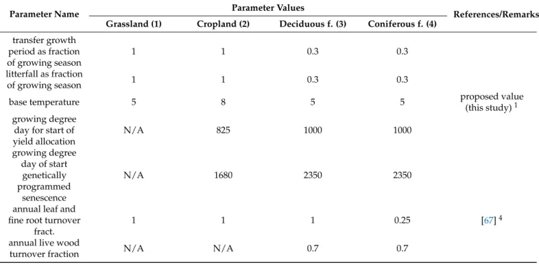
Table A1.List of ecophysiological parameters for the Biome-BGCMuSo v4.0 model used in this study. Values for Grassland, Cropland and Deciduous forest are from Hidy et al. (2016) [34], with some parameters adjusted according to specified references or proposed for the purpose of this study. Parameters for Coniferous forests are based on parameters for Deciduous forests and adjusted according to specified references. Superscripts in the Reference column refer to the vegetation type (1Grassland,2Cropland,3Deciduous forest,4Coniferous forest).
Parameter Name Parameter Values
References/Remarks Grassland (1) Cropland (2) Deciduous f. (3) Coniferous f. (4)
transfer growth period as fraction of growing season
1 1 0.3 0.3
litterfall as fraction
of growing season 1 1 0.3 0.3
base temperature 5 8 5 5 proposed value
(this study)1 growing degree
day for start of yield allocation
N/A 825 1000 1000
growing degree day of start genetically programmed
senescence
N/A 1680 2350 2350
annual leaf and fine root turnover
fract.
1 1 1 0.25 [67]4
annual live wood
turnover fraction N/A N/A 0.7 0.7
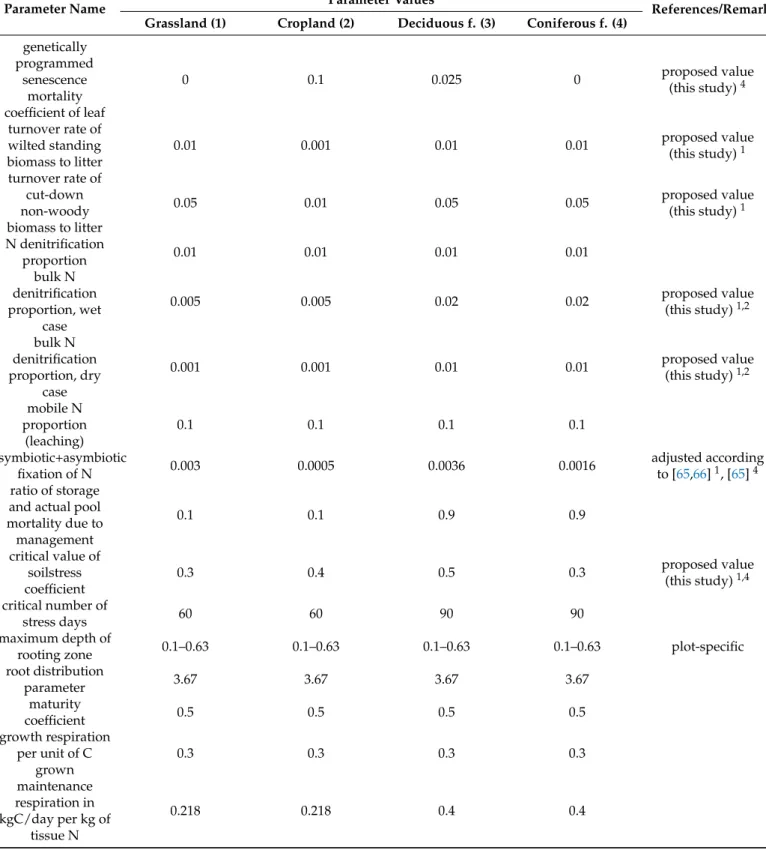
Table A1.Cont.
Parameter Name Parameter Values
References/Remarks Grassland (1) Cropland (2) Deciduous f. (3) Coniferous f. (4)
annual whole-plant mortality fraction
0.05 0.02 0.02 0.005 [39]4
annual fire
mortality fraction 0 0 0 0
new fine root C:
new leaf C 2.5 1.02 0.95 1 adjusted according
to [63]1, [37]4 new fruit C: new
leaf C 0 0.56 0.14 0 proposed value
(this study)4 new softstem C:
new leaf C 0.5 2.05 N/A N/A
new woody stem
C: new leaf C N/A N/A 1.42 2.2 [39]4
new live wood C:
new total wood C N/A N/A 0.16 0.1 [36]4
new coarse root C:
new stem C N/A N/A 0.26 0.3 [36]4
current growth
proportion 0.5 1 0.5 0.5 proposed value
(this study)1
C:N of leaves 25 38 24.5 42 adjusted according
to [64]2, [39]4
C:N of leaf litter 45 65 47.5 93 [39]4
C:N of fine roots 50 42 43 58 [39]4
C:N of fruit 25 50 33 0 proposed value
(this study)4
C:N of softstem 25 85 N/A N/A
C:N of live wood N/A N/A 73.5 50 [39]4
C:N of dead wood N/A N/A 451 729 [67]4
leaf litter labile
proportion 0.68 0.68 0.2 0.32 [36]4
leaf litter cellulose
proportion 0.23 0.23 0.56 0.44 [36]4
fine root litter
labile proportion 0.34 0.34 0.34 0.30 [36]4
fine root litter cellulose proportion
0.44 0.44 0.44 0.45 [36]4
fruit litter labile
proportion N/A 0.68 0.3 0 proposed value
(this study)4 fruit litter cellulose
proportion N/A 0.23 0.29 0 proposed value
(this study)4 softstem litter
labile proportion 0.68 0.68 N/A N/A
softstem litter cellulose proportion
0.23 0.23 N/A N/A
dead wood cellulose proportion
N/A N/A 0.75 0.76 [36]4
Table A1.Cont.
Parameter Name Parameter Values
References/Remarks Grassland (1) Cropland (2) Deciduous f. (3) Coniferous f. (4)
canopy water interception
coefficient
0.01 0.01 0.038 0.041 [67]4
canopy light extinction coefficient
0.5 0.6 0.54 0.5 proposed value
(this study)1, [67]4 all-sided to
projected leaf area ratio
2 2 2 2.6 [39]4
canopy average
specific leaf area 49 43.3 34.5 12 [67]4
ratio of shaded specific leaf area:sunlit specific
leaf area
2 2 2 2
fraction of leaf N
in Rubisco 0.2 0.39 0.088 0.04
proposed value (this study)1,2, [67]
4
fraction of leaf N
in PeP carboxylase N/A 0.03 N/A N/A
maximum stomatal conductance
0.004 0.012 0.0024 0.003 proposed value
(this study)1, [36]4 cuticular
conductance 0.00006 0.00006 0.00006 0.00001 [36]4
boundary layer
conductance 0.04 0.04 0.005 0.08 [36]4
relative soil water content limitation1 (proportion to field capacity value)
1 1 1 1 proposed value
(this study)3,4 relative soil water
content limitation 2 (proportion to saturation capacity
value)
0.99 0.99 1 1 proposed value
(this study)3,4
vapour pressure deficit: start of
conductance reduction
1000 1000 200 930 [67]4
vapour pressure deficit: complete conductance
reduction
5000 5000 2550 4100 proposed value
(this study)1, [67]4 senescence
mortality coefficient of aboveground plant
material
0.05 0.05 0.01 0 proposed value
(this study)4
senescence mortality coefficient of belowground plant
material
0.01 0.01 0.01 0 proposed value
(this study)4
Table A1.Cont.
Parameter Name Parameter Values
References/Remarks Grassland (1) Cropland (2) Deciduous f. (3) Coniferous f. (4)
genetically programmed
senescence mortality coefficient of leaf
0 0.1 0.025 0 proposed value
(this study)4
turnover rate of wilted standing biomass to litter
0.01 0.001 0.01 0.01 proposed value
(this study)1 turnover rate of
cut-down non-woody biomass to litter
0.05 0.01 0.05 0.05 proposed value
(this study)1 N denitrification
proportion 0.01 0.01 0.01 0.01
bulk N denitrification proportion, wet
case
0.005 0.005 0.02 0.02 proposed value
(this study)1,2 bulk N
denitrification proportion, dry
case
0.001 0.001 0.01 0.01 proposed value
(this study)1,2 mobile N
proportion (leaching)
0.1 0.1 0.1 0.1
symbiotic+asymbiotic
fixation of N 0.003 0.0005 0.0036 0.0016 adjusted according
to [65,66]1, [65]4 ratio of storage
and actual pool mortality due to
management
0.1 0.1 0.9 0.9
critical value of soilstress coefficient
0.3 0.4 0.5 0.3 proposed value
(this study)1,4 critical number of
stress days 60 60 90 90
maximum depth of
rooting zone 0.1–0.63 0.1–0.63 0.1–0.63 0.1–0.63 plot-specific
root distribution
parameter 3.67 3.67 3.67 3.67
maturity
coefficient 0.5 0.5 0.5 0.5
growth respiration per unit of C
grown
0.3 0.3 0.3 0.3
maintenance respiration in kgC/day per kg of
tissue N
0.218 0.218 0.4 0.4
Table A2.Description of management activities for different land-use categories simulated with the Biome-BGCMuSo model.
Land-Use Category Management Activity DOY Description
Deciduous forests
Coniferous forests Thinning * 30 2.1% y−1
3% y−1
Grassland fertilising 100, 190 30 + 30 kg N ha−1y−1
animal manure (2% N, 40% C)
Mowing 150, 200 75% plant material
Annual cropland
Planting 105 25 kg ha−1
fertilising 91, 145, 288
60 + 40 + 50 kg N ha−1y−1 70% chemical fertiliser (47%
N, 5% C) 30% animal manure
Harvesting 273 50% plant material
Ploughing 300 down to 30 cm
* Deciduous forests in Croatia are even-aged managed, with thinnings of 15% performed every 10 years and with regeneration cuts (2–3 cuts) performed during the last 10 years of the rotation period. In order to perform spatial modelling, we needed thinnings and regeneration cuts distributed among different locations. In the absence of this information, we estimated average annual thinning intensity to ensure evenly distributed thinning at the spatial scale. If we assume a rotation period of 140 years (i.e., prescribed rotation for pedunculate oak), annual thinning intensity should account for 1.5% thinning rate during a 130 year period and 100% regeneration cut during whole rotation period, which sums to 2.1%. Coniferous forests are uneven-aged managed with thinning of 30% performed every 10 years, i.e., average annual thinning intensity is 3%.
Figure A1.Comparison of measured and modelled soil organic carbon stocks down to 30 cm in different land-use categories with respect to biogeographical regions. Asterisk indicates statistically significant difference (p< 0.01) between measured and modelled data at the land use×biogeographical region level.
Figure A2.Residual analysis for different land-use categories.
References
1. UN (United Nations).Kyoto Protocol to the United Nations Framework Convention on Climate Change; United Nations: Kyoto, Japan, 1997; pp. 1–21. Available online:https://unfccc.int/resource/docs/cop3/07a01.pdf(accessed on 23 July 2021).
2. UN (United Nations).Paris Agreement; United Nations: Paris, France, 2015; pp. 1–27. Available online:https://undocs.org/en/
FCCC/CP/2015/10/Add.1(accessed on 23 July 2021).
3. EC (European Commission).Communication from the Commission to the European Parliament, the European Council, the Council, the European Economic and Social Committee and the Committee of the Regions-The European Green Deal; European Commission: Brussels, Belgium, 2019; pp. 1–24.
4. Batjes, N.H. Total C and N in soils of the world.Eur. J. Soil Sci.1996,47, 151–163. [CrossRef]
5. Scharlemann, J.P.W.; Tanner, E.V.J.; Hiederer, R.; Kapos, V. Global soil carbon: Understanding and managing the largest terrestrial carbon pool.Carbon Manag.2014,5, 81–91. [CrossRef]
6. Crowther, T.W.; Todd-Brown, K.E.O.; Rowe, C.W.; Wieder, W.R.; Carey, J.C.; Machmuller, M.B.; Snoek, B.L.; Fang, S.; Zhou, G.;
Allison, S.D.; et al. Quantifying global soil carbon losses in response to warming.Nature2016,540, 104–108. [CrossRef] [PubMed]
7. Rustad, L.E.; Campbell, J.L.; Marion, G.M.; Norby, R.J.; Mitchell, M.J.; Hartley, A.E.; Cornelissen, J.H.C.; Gurevitch, J. Gcte-News.
A meta-analysis of the response of soil respiration, net nitrogen mineralization, and aboveground plant growth to experimental ecosystem warming.Oecologia2001,126, 543–562. [CrossRef] [PubMed]
8. Melillo, J.M.; Steudler, P.A.; Aber, J.D.; Newkirk, K.; Lux, H.; Bowles, F.P.; Catricala, C.; Magill, A.; Ahrens, T.; Morrisseau, S. Soil warming and carbon-cycle feedbacks to the climate system.Science2002,298, 2173–2176. [CrossRef] [PubMed]
9. Fyson, C.L.; Jeffery, M.L. Ambiguity in the land use component of mitigation contributions toward the Paris agreement goals.
Earths Future2019,7, 873–891. [CrossRef]
10. IPCC GPG (The Intergovernmental Panel on Climate Change Good Practice Guidelines).Guidelines for National Greenhouse Gas Inventories; Eggleston, H.S., Buendia, L., Miwa, K., Ngara, T., Tanabe, K., Eds.; National Greenhouse Gas Inventories Programme, IGES: Kanagawa, Japan, 2006.
11. Jenkinson, D.S.; Coleman, K. The turnover of organic carbon in subsoils. Part 2. Modelling carbon turnover.Eur. J. Soil Sci.2008, 59, 400–413. [CrossRef]
12. UK NIR. United Kingdom National Inventory Report 2020. Available online:https://unfccc.int/documents/225987(accessed on 23 July 2021).
13. Liski, J.; Palosuo, T.; Peltoniemi, M.; Sievanen, R. Carbon and decomposition model Yasso for forest soils.Ecol. Modell.2005, 189, 168–182. [CrossRef]
14. Alvaro-Fuentes, J.; Easter, M.; Cantero-Martinez, C.; Paustian, K. Modelling soil organic carbon stocks and their changes in the northeast of Spain.Eur. J. Soil Sci.2011,62, 685–695. [CrossRef]
15. CH NIR. Swiss National Inventory Report 2020. Available online: https://unfccc.int/documents/224855(accessed on 23 July 2021).
16. FI NIR. Finnish National Inventory Report 2020. Available online: https://unfccc.int/documents/219060 (accessed on 23 July 2021).
17. Parton, J.W. The century model. InEvaluation of Soil Organic Matter Models; Powlson, D.S., Smith, P., Smith, J.U., Eds.; Springer:
Berlin/Heidelberg, Germany, 1996; pp. 283–291.
18. Falloon, P.; Smith, P. Accounting for changes in soil carbon under the Kyoto Protocol: Need for improved long-term data sets to reduce uncertainty in model projections.Soil Use Manag.2003,19, 265–269. [CrossRef]
19. Hararuk, O.; Xia, J.Y.; Luo, Y.Q. Evaluation and improvement of a global land model against soil carbon data using a Bayesian Markov chain Monte Carlo method.J. Geophys. Res. Biogeosci.2014,119, 403–417. [CrossRef]
20. Tupek, B.; Launiainen, S.; Peltoniemi, M.; Sievanen, R.; Perttunen, J.; Kulmala, L.; Penttila, T.; Lindroos, A.J.; Hashimoto, S.;
Lehtonen, A. Evaluating CENTURY and Yasso soil carbon models for CO2emissions and organic carbon stocks of boreal forest soil with Bayesian multi-model inference.Eur. J. Soil Sci.2019,70, 847–858.
21. Luo, Y.; Zhou, X.Soil Respiration and the Environment; Elsevier: Amsterdam, The Netherlands, 2006; p. 316.
22. Campbell, E.E.; Paustian, K. Current developments in soil organic matter modelling and the expansion of model applications:
A review.Environ. Res. Lett.2015,10, 123004. [CrossRef]
23. Parton, W.; Del Grosso, S.J.; Plante, A.F.; Adair, E.C.; Lutz, S.M. Modelling the dynamics of soil organic matter and nutrient cycling. InSoil Microbiology, Ecology, and Biochemistry, 4th ed.; Paul, E.A., Ed.; Elsevier: Amsterdam, The Netherlands, 2015;
pp. 505–537.
24. Keel, S.G.; Leifeld, J.; Mayer, J.; Taghizadeh-Toosi, A.; Olesen, J.E. Large uncertainty in soil carbon modelling related to method of calculation of plant carbon input in agricultural systems.Eur. J. Soil Sci.2017,68, 953–963. [CrossRef]
25. Ostle, N.J.; Levy, P.E.; Evans, C.D.; Smith, P. UK land use and soil carbon sequestration. Land Use Policy2009,26, S274–S283.
[CrossRef]
26. Poeplau, C.; Don, A.; Vesterdal, L.; Leifeld, J.; Van Wesemael, B.; Schumacher, J.; Gensior, A. Temporal dynamics of soil organic carbon after land-use change in the temperate zone-carbon response functions as a model approach. Glob. Change Biol.2011, 17, 2415–2427. [CrossRef]
27. Johnson, D.W.; Curtis, P.S. Effects of forest management on soil C and N storage: Meta analysis. For. Ecol Manag. 2001,140, 227–238. [CrossRef]
28. Chen, L.C.; Wang, S.L.; Wang, Q.K. Ecosystem carbon stocks in a forest chronosequence in Hunan Province, South China.Plant Soil2016,409, 217–228. [CrossRef]
29. Ostrogovi´c Sever, M.Z.; Alberti, G.; Delle Vedove, G.; Marjanovi´c, H. Temporal Evolution of carbon stocks, fluxes and carbon balance in pedunculate oak chronosequence under close-to-nature forest management.Forests2019,10, 814. [CrossRef]
30. Smith, J.; Smith, P.; Wattenbach, M.; Zaehle, S.; Hiederer, R.; Jones, R.J.A.; Montanarella, L.; Rounsevell, M.D.A.; Reginster, I.;
Ewert, F. Projected changes in mineral soil carbon of European croplands and grasslands, 1990–2080.Glob. Change Biol.2005, 11, 2141–2152. [CrossRef]
31. Mondini, C.; Coleman, K.; Whitmore, A.P. Spatially explicit modelling of changes in soil organic C in agricultural soils in Italy, 2001–2100: Potential for compost amendment.Agric. Ecosyst. Environ.2012,153, 24–32. [CrossRef]
32. Munoz-Rojas, M.; Jordan, A.; Zavala, L.M.; Gonzalez-Penaloza, F.A.; De la Rosa, D.; Pino-Mejias, R.; Anaya-Romero, M. Modelling soil organic carbon stocks in global change scenarios: A CarboSOIL application.Biogeosciences2013,10, 8253–8268. [CrossRef]
33. Running, S.W.; Hunt, E.R.J. Generalization of a forest ecosystem process model for other biomes, BIOME-BGC, and an application for global-scale models. InScaling Physiological Processes: Leaf to Globe; Ehleringer, J.R., Field, C., Eds.; Academic Press: San Diego, CA, USA, 1993; pp. 141–158.
34. Hidy, D.; Barcza, Z.; Marjanovic, H.; Sever, M.Z.O.; Dobor, L.; Gelybo, G.; Fodor, N.; Pinter, K.; Churkina, G.; Running, S.; et al.
Terrestrial ecosystem process model Biome-BGCMuSo v4.0: Summary of improvements and new modeling possibilities.Geosci.
Model Dev.2016,9, 4405–4437. [CrossRef]
35. Pietsch, S.A.; Hasenauer, H. Using mechanistic modeling within forest ecosystem restoration.For. Ecol. Manag.2002,159, 111–131.
[CrossRef]
![Table 1. Area of land-use categories in Republic of Croatia in 2016 according to HR NIR 2020 [59].](https://thumb-eu.123doks.com/thumbv2/9dokorg/766079.33745/4.892.254.839.171.407/table-area-land-categories-republic-croatia-according-nir.webp)