MTA doktori értekezés
CELL AND LIPID MEMBRANE STRUCTURES.
EFFECTS OF ELECTRIC, THERMAL AND CHEMICAL INTERACTIONS
István P. Sugár
New York, 2010
Table of Contents
Introductory Notes 5
1. Effect of electric field on the structure of cell membranes 1.1. Stochastic theory of cell electroporation
1.1.1. Introduction 6 1.1.2. The model 6
1.1.2.1. General pore structure 7 1.1.2.2. The stochastic variable 7 1.1.2.3. Transition probabilities 8
1.1.2.4. Free energy function at zero electric field 9
1.1.2.5. Free energy function in the presence of an electric field 9 1.1.2.6. Master equations of electroporation 10
1.1.3. Results and discussion 11 1.1.3.1. Stationary solutions 11
1.1.3.1.1. Reversible electroporation in stable membranes 13 1.1.3.2. Quasi-stationary solutions 13
1.1.3.2.1. Mechanical breakdown, reversible and irreversible electroporation 14 1.1.3.3. Nonstationary solutions 14
1.1.3.3.1. Time delay of mechanical breakdown – Membrane lifetime 15 1.1.3.3.2. Time delay of electroporation 16
1.1.3.4. Transition kinetics 18
1.1.3.4.1. Poreless Porous transition 18 1.1.3.5. Membrane rupture 19
1.1.3.5.1. Resealing process 19
1.2. Phenomenological theory of low voltage electroporation 1.2.1. Introduction 20
1.2.2. Model 23
1.2.2.1. Geometry of the model of low voltage electroporator 23
1.2.2.2. Laplace equation of the model of low voltage electroporator 25 1.2.2.2.1. Boundary conditions 25
1.2.2.2.2. Laplace equation in inhomogeneous medium 26 1.2.2.2.3. The matching conditions 26
1.2.2.2.4. Numerical solution of the Laplace equation 26 1.2.3. Results 26
1.2.4. Discussion 29
1.2.4.1. Transmembrane voltage 29
1.2.4.2. Distribution of electropores 32 1.2.4.3. Electric field and potential 33 1.2.4.4. Minimal applied voltage 35 1.2.4.5. Efficiency of electroporation 36 1.2.5. Conclusions 37
1.2.6. Appendix 1 - Joule Heating in LVEP 37
1.2.7. Appendix 2 - Estimation of the thickness of the narrow passage 39
1.2.8. Appendix 3 - On the deviations of the model's geometry from the electroporator's geometry 40
2. Effect of temperature and composition on the structure of two-component lipid membranes
2.1. Introduction 42
2.2. Lattice model of DMPC/DSPC bilayers 43 2.2.1. Lattice geometry, states and configuration 43 2.2.2. Configurational energy and degeneracy 45 2.2.3. Configurational probability 46
2.2.4. Steps in the Monte Carlo simulations 46 2.2.5. Generation of trial configurations 47 2.2.5.1. Local state alteration 47
2.2.5.2. Exchanging different molecules 47
2.2.5.3. Reorientation of a pair of nearest-neighbor molecules 47 2.2.6. Decision making 47
2.2.7. Defining the Monte Carlo cycle 48 2.2.8. Global state alteration 48
2.2.9. Determination of the model parameters 49 2.3. Results and discussion 50
2.3.1. System size and type of transition 50
2.3.2. Excess heat capacity curves and melting curves 52 2.3.3. Domain structure of the membranes 55
2.3.4. Cluster statistics 56 2.3.5. Cluster number 58 2.3.6. Cluster percolation 59 2.3.7. „Small‟ clusters 61
2.3.8. Membrane permeability 63
2.4. Conclusions 65
3. Lipid monolayer structure controls protein adsorption. Model of peripheral protein adsorption to the water/lipid interface
3.1. Introduction 66 3.2. The model 68
3.2.1. Structure of PL/DG monolayers 68
3.2.2. Free area and discrete molecular area 69
3.2.3. Characterization of monolayer configuration 70 3.2.4. The normalized initial adsorption rate 71
3.2.5. Probability density of free area under a colipase - pf 72
3.2.6. Probability density of discrete area of uncomplexed molecules under a colipase - pu 73
3.2.7. Numerical integration 74 3.3. Results and discussion 74
3.3.1. Protein adsorption to POPC monolayers 74
3.3.2. Protein adsorption to DO/POPC monolayers 75
3.3.3. Protein adsorption to DO/POPC monolayers at collapse pressure 77 3.4. Conclusions 79
3.5. Appendix 1 - Definitions of frequently used symbols 79
3.6. Appendix 2 - The probability density that the free area of n lipid molecules is f 80 3.7. Appendix 3 - Calculation of ACP and q 81
3.8. Appendix 4 82
3.8.1. Incomplete beta function and the binomial distribution 82 3.8.2. Extensions of the incomplete beta function 84
4. Membrane geometry regulates intercellular communication. Model of autocrine/paracrine signaling in epithelial layer
4.1. Introduction 86 4.2. Model 87
4.2.1. Model geometry 87
4.2.2. Diffusion equation of the model 89
4.2.3. Numerical Solution of the Diffusion Equation 90 4.3. Results and discussion 92
4.3.1. Plot types of trapping site distributions 92
4.3.2. Ligands emission from the top of a microvillus 93
4.3.2.1. Geometrical parameters g and d decrease simultaneously, while g d 93 4.3.2.2. Geometrical parameter g decreases gradually, while d remains constant 95 4.3.3. Ligand emission from the side of a microvillus 97
4.3.4. Probability of autocrine signaling 99 4.4. Conclusions 102
4.5. Appendix 1 102 4.6. Appendix 2 105
4.7. Appendix 3 - Calculating the area accessible for ligand absorption 107 5. References
5.1. References to Chapter 1.1. 109 5.2. References to Chapter 1.2. 109 5.3. References to Chapter 2. 110 5.4. References to Chapter 3. 112 5.5. References to Chapter 4. 113
Introductory Notes
The structure of a cell membrane determines its functions. By changing the external conditions one can change the membrane structure and consequently its functions. The work presented here intends to demonstrate these simple statements on four different membranes: single cell membrane, lipid vesicle, lipid monolayer and epithelial layer.
We reveal the physical mechanism of how external fields, such as electric field or temperature, are able to change the membrane structure (Sec. 1, 2). In these cases the external conditions result in the structural and consequently the functional changes. In other cases the cell itself can change either the composition or geometry of its membrane that result in functional changes (Sec. 4).
The theoretical models presented here are so called minimal models. The assumptions made by these models are both physically and biologically plausible and absolutely necessary for the correct description of the observed phenomena. As a consequence the number of model parameters is minimal and the parameters have explicit physical meaning. The unique feature of this approach is that experimental data are utilized to estimate the values of the model parameters. In contrast to ab-initio calculations development of these minimal models assume close collaboration with the experimentalists.
The mathematical approach utilized in the model depends on the studied system and the questions that we intend to answer. The kinetics of electropore formation is described by using the theory of stochastic processes (Sec. 1.1). Membrane heterogeneity or
equilibrium lateral distribution of membrane components is described by means of Monte Carlo simulation techniques (Sec. 2). In the cases of systems with complicated overall geometries, such as the distorted cell shape in low voltage electroporator or the rugged surface of the epithelial layer, we use numerical methods to solve the respective partial differential equations (Sec. 1.2, 4).
A model that is able to describe a broad range of experiments has predictive power. One becomes able to calculate yet un-measured or currently un-measurable properties of the system. For example the model of two-component phospholipid membranes reveals the size distribution and even the inner structure of the compositional clusters (Sec. 2), while experimentally we are able to detect only the large clusters in the micrometer range.
It is important to emphasize that besides the purely theoretical values the presented work can lead to applications in medical- and biotechnology. For example low voltage
electroporation, that is discussed in Sec. 1.2 is the most promising method for ex-vivo cell transfection by foreign gene.
1. Effect of electric field on the structure of cell membranes 1.1 Stochastic theory of cell electroporation
1.1.1. Introduction
In 1972 Neumann and Rosenheck1 discovered the permeabilization of lipid vesicles when a certain threshold value of the field strength is exceeded. The electrically induced permeability increase, called electroporation, leads to transient exchange of matter across the perturbed membrane structures. An important aspect of electric field effects on membrane structures is the artificial transfer of macromolecules or particles into the interior of biological cells and organelles. Super-critical electric fields can be used to transfect culture cells in suspension with foreign genes.
Two basic mechanisms have been suggested to describe the experimentally observed properties of electroporation: the electromechanical model and the statistical model of pore expansion. These models have been reviewed by Dimitrov and Jain2. This chapter develops an exactly solvable statistical model of electroporation for one-component planar lipid bilayer membrane. At zero electric field, the membrane is populated with microscopic pores by the fluctuation clustering of vacancies (i.e. lipid molecule-free sites) in the bilayer. Under the effect of transmembrane electric field, the average pore size increases. The driving force of the electric field-mediated pore opening is associated with the enhancement of the electric polarization of the solvent molecules during their transfer from the bulk solvent space to the region of the larger electric field spreading from the pore wall into the solution of the pore interior (see Fig.1 and Sugar and Neumann3; Powell et al.4).
The characteristic features of the present model are the following: (1) the model results are valid independently from the molecular details of the pore structure; (2) the
phenomena of elelectroporation are described quantitatively in the case of both stable and metastable planar bilayer membranes when the transmembrane voltage is changed
stepwise; (3) the uniform description of reversible and irreversible electroporation and mechanical breakdown is presented; exact solutions of the stochastic equations of the electroporation are determined; (5) the pores are considered to be independent from each other. The consequences of pore-pore interaction, pore coalescence, and integral proteins are discussed elsewhere5. The results of the model are compared with the available experimental data, such as membrane lifetime, critical transmembrane voltage, and membrane conductance during the resealing process.
1.1.2. Model
On the basis of energetic considerations, different pore structures have been proposed:
hydrophobic pore and inverted pore model6, and periodic block model3. The description of the present electroporation model does not require a detailed knowledge of the pore structure.
1.1.2.1. General Pore Structure
The following general pore properties are assumed in the model (Fig. 1): (1) A common feature of every pore model is that the water-filled pore interior is surrounded by the pore wall, and the pore wall is surrounded by the bulk bilayer lipid membrane. The structure of the lipid molecules within the pore wall is different from the bilayer structure of the bulk membrane. Consequently the specific energy of the pore wall is different from that of the bulk membrane. (2) During the pore opening and closing process, the number of lipid molecules within the pore wall increases and decreases, respectively. In the case of planar membranes, lipid transfer into the pore wall takes place simultaneously from both monolayers of the bilayer membrane. However, it is assumed that the sites of these two transfer processes along the pore circumference are independent of each other.
Figure 1. Side and top views of the general pore structure. The water-filled pore interior (w) is surrounded by the pore wall (shaded area), which in turn is surrounded by the bulk bilayer lipid membrane. r is the pore radius; r* is the thickness of the region of the larger electric field; solid and dashed arrows show possible sites of lipid transfer from the upper and lower monolayer of the bilayer to the pore wall, respectively
1.1.2.2. The Stochastic Variable
Assumig circular pore geometry, both the state of the pore and the process of electroporation can be described by one stochastic variable, a. This variable is
proportional to the number of lipid molecules in the pore wall. The stochastic variable a and the pore radius r are related by:
(2 / )
a INT r l (1)
where INT integer part of a numerical value p.qrs, e.g., INT p qrs( . ) p, and l is the characteristic length along the pore circumference. The value of the characteristic length depends on the molecular structure of the pore wall. For example, in the case of the periodic block model3, l is twice the cross-sectional diameter of a lipid molecule.
The opening and closing process of a single membrane pore may be treated as a stochastic process in terms of a Markov chain7. The general stochastic state transitions are given by the scheme:
0 1 1
1 2 1
0 1 2 1 1
a a
a a
w w w w
w w w w
a a a
Where wa and wa represent the “rate constants” or transition probabilities per unit time for the a (a 1) pore opening step and a (a 1)pore closing step, respectively.
Within the framework of this general scheme, the physics of electroporation is
concentrated in the functions of the transition probabilities. In the next three sections, the transition probabilities in the function of the external electric field strength are
determined and then the stochastic equations of the electroporation are constructed.
1.1.2.3. Transition Probabilities
Denoting by t a small time interval within which one state transition a (a 1) occurs, the transition probability of this state change is given by
( / ) exp [( *( 0.5) ( )) / ]
wa t t G a G a kT (2)
And the transition probability of a (a 1)process is
1 ( / ) exp [( *( 0.5) ( 1)) / ]
wa t t G a G a kT (3)
where is the characteristic time, 1/ is the transition frequency as the number of trials per unit time, T is the absolute temperature, k is the Boltzmann constant,
( ) ( ) (0)
G a G a G is the Gibbs free energy change of the membrane/solution system in the presence of an electric field when a single pore of state a forms in the bilayer, and
* ( 0.5)
G a is the free energy change when an activated pore structure forms between state a and a+1 in the bilayer. The activated pore structure is different from the structure of the neighbor states. It‟s structural energy is higher by than the average of the structural energies of the neighbor states. For the sake of simplicity is independent of the pore state. The activation Gibbs free energies are given by
*( 0.5) ( ) ln( [ 0.5])2 ( 0.5) ( )
G a G a kT a G a G a (4)
*(0.5) (0) (0.5) (0)
G G G G (5)
The second term in Eq.4 contains the activation entropy. The transfer of lipid molecules to or from the pore wall from or to one layer of the bilayer can take place at different sites. The number of possible sites, [a 0.5], is proportional to the pore circumference
(see Eq.1); is the proportionality constant. Since the sites of transfer from or to the two layers of the bilayer to or from the pore wall are independent (see Section 1.1.2.1), the square of [a 0.5] gives the thermodynamic probability of the activated pore between a and a+1 states.
1.1.2.4. Free Energy Function at Zero Electric Field
According to the nucleation theory of bilayer stability8,9 at zero electric field, the free energy change of the membrane/solution system when a single pore of radius r forms is
2
( ) ( b s) / 0 2
G r r A r (6)
Where s and b are the chemical potential of the monomer lipid molecule in the solution (s) and in the bilayer membrane (b), respectively; A0 is the cross-sectional area of a lipid molecule. The second term is the energy expended on the creation of the pore wall; is the energy of the pore wall per unit length. When ( b s) 0, the free energy change G r( ) increases with increasing pore radius. In this case, pores of any size tend to shrink and the bilayer is stable with respect to rupture. However, in the case of 0 the G r( ) function decreases from a certain pore radius rc; if r rc the pore tends to shrink and the bilayer is metastable with respect to rupture; if r rc the pore can grow spontaneously and the bilayer is unstable.
The chemical potential difference, and consequently the bilayer stability, depends on the monomer lipid concentration C in the solution. Denoting Ce as the concentration where
0 and denoting CMC as the critical micelle concentration8, then the bilayer is stable when Ce C CMC. The bilayer is metastable when C Ce CMC or
C CMC Ce.
Although experimental data are not available on stable planar bilayers, the model calculations were performed for stable systems. These calculations have biological relevance because the electroporation of the stable planar bilayer should be analogous to the electroporation of giant lipid vesicles10 or to the electroporation of the protein-free domains of cell membranes (see Section 1.1.3.1).
1.1.2.5. Free Energy Function in the Presence of an Electric Field
In the presence of a transmembrane electric field, one has to introduce additional energy terms into the free energy function (Eq.6) describing the change in the electric
polarization energy of the system Gel( )r when a single pore of radius r forms in the bilayer3. If r r*
2 2
( ) 0.5 (0 )
el m w m
G r r dE (7)
If r r*
2 2 2 2
( ) 0.5 0 [( 1) ( 1)( { *} )]
el m m w
G r dE r r r r (8)
In Eq.7 and 8, d is the bilayer thickness, Em is the electric field strength in the bilayer, and 0, m, and w are the vacuum dielectric permittivity, relative dielectric permittivity of the membrane, and relative dielectric permittivity of water, respectively. During the derivation of Eqs.7 and 8, the following assumptions were made.
(1) At higher ionic strengths (>0.1M), the electric conductivity of the aqueous
solution is so much larger than that of the planar bilayer that the applied voltage U only drops across the bilayer. In terms of the constant field approximation, the average field in the bilayer is given by Em U d/ ; the field strength in the bulk electrolyte may be approximated by Es 0.
(2) The electric field within the solvent-filled pore is inhomogeneous, decreasing from the value Em( U d/ ) at the pore wall/solvent interface toward the pore center. In the layer of solvent molecules adjacent to the inner cylindrical part of the pore wall of thickness r*, the field intensity is approximated by Ep Em (Fig.1). For larger pores where r r*, the electric field strength in the central region of radius r r* is considered to be Es 0. For small pores where r r*, the homogeneous field approximation Ep Em holds. According to Jordan11, at 1M ionic strength the electric field becomes highly inhomogeneous if r d/ 5. For these conditions, the relation r* d/ 5 specifies the largest pore size to which the small-pore field approximation Ep Em may be applied. In the case of
oxidized cholesterol membranes, d 3.3nm (Benz et al.12). Thus, r* 0.86nm at 0.1M ionic strength; r* increases with decreasing ionic strength11.
Introducing the pore state a, defined in Eq.1, into Eqs.6-8, the Gibbs free energy function is given by G a( ) G a( ) G ael( ); see the transition probability functions in Eqs.2-5.
Eqs. 2-8 permit the calculation of the transition probabilities as a function of the pore state and transmembrane voltage. For this purpose, the numerical values characteristic to the oxidized cholesterol bilayer we utilized12; 1.25 10 11N (Abidor et al.6), l 1.8nm (Sugar and Neumann3), T=313K, m 2.1, w 80. The calculations were performed with three values of /A0( g): -0.001, 0.0, and 0.001 N/m. These values are typical for stable and metastable bilayers13, respectively.
1.1.2.6. Master Equations of Electroporation The probability
,0( )
Pa a t t of occurrence of a pore state a at time t tif the state is a0 at time t 0 is given by
0 0 0 0
, ( ) 1 1, ( ) 1 1, ( ) (1 [ ] ) , ( )
a a a a a a a a a a a a
P t t w tP t w tP t w w t P t (9)
This difference equation may be transformed into the forward master equation7:
0 0 0 0
, ( ) / 1 1, ( ) 1 1, ( ) [ ] , ( )
a a a a a a a a a a a a
dP t dt w P t w P t w w P t (10)
1.1.3. Results and Discussion
Since the transition probabilities
w
a andw
a in the master equation of theelectroporation (Eq.10) are nonlinear functions of the pore state a, no general solution is possible. However, one can determine the exact stationary and quasi-stationary solutions, the lifetime of the metastable membrane, the kinetics of pore opening and closing as well as other parameters.
1.1.3.1. Stationary Solutions
If the pore state a is confined in the (0,a*) interval, the stationary pore size distribution
,0( )
Pa a t can be determined by means of Eq.11 in Table 1. The different solutions of the master equations (Eq.10) in Table 1 were taken from Goel and Richter-Dyn7. Table 1. Expressions for the Equilibrium Distribution
,0( )
Pa a and for the First Passage Time
0
(1) ,
Ta a
0 a0 a*
0
*
0 1 1 0 1 1
,
1 2 1 1 2
( )
a
a i
a a
a i i
w w w w w w
P w w w w w w (11) 0 a0 a
0 0
1
(1) 1
, 1,
0
a i
a a n n i
i a n
T w (12) 0 a a0 a*
0 0
0
* 1 * 1
(1) 1 1
, 1, , , 1, ,
1 1 1
a i a i
a a n n i a n a a n n i a n
i a n a i a n a
T w R R w R (13)
0 a a0 0
0
(1)
, 1,
1 a
a a i i
i a
T M (14)
1 ,
1
i i j
i j
i i j
w w w
w w w if i j and
, 1 1
i i
0 0
* 1 * 1
, 1, 1,
a a
a a a i a i
i a i a
R
1 1,
1 1 2
1 i i i
i i
i i i i i i
w w w
M w w w w w w
Physically, the upper limit of the pore size is comparable to the membrane size itself, i.e., a* is a good approximation. In the case of stable membranes, the infinite sum in Eq.11 is convergent. The logarithm of the pore state distributions are shown in Fig. 2a at different transmembrane voltages. At subcritical electric fields (U Ucrs 0.4 )V , the pore size distribution is unimodal with a cusplike maximum at a=0. This maximum of the distribution curve defines a phase termed the poreless phase of the stable bilayer. At supercritical electric fields (U Ucrs 0.4 )V , the pore size distribution has two maxima:
one at a=0 represents the poreless phase and one at a>0 defines the so-called porous
phase of the membrane. When the maximum belonging to the porous phase exceeds the cusplike maximum at the poreless phase, the membrane lipids form pore walls almost exclusively. In the frame of our independent pore model, this loose net structure of the membrane is still stable. This is a transmembrane voltage-induced phase transition of the membrane from the poreless phase into the porous phase.
Figure 2. Stationary and quasi- stationary pore state distributions at different transmembrane voltages.
a) Stable membrane (dashed and dotted line: U Ucrs , solid line: U Ucrs ; b) metastable membrane (solid line: quasi- stationary pore state distribution.
Beginning of dashed line defines a* - the limit state of the quasi-stationary pores.)
Figure 3. Characteristic quantities of electroporation as a function of transmembrane voltage. a),b) Stable membranes; c) metastable membrane.
Solid line: average pore state calculated by Eq.15; dashed line: pore state
fluctuation calculated by Eq.16; dotted line: the most probable state of the porous phase; dash-dotted line: limit state of quasi-stationary pores, a*. In Fig. 3a and b, characteristic values of the pore state distribution curves are plotted as a function of transmembrane voltage. The solid lines represent the average pore state calculated by
0
* , 0
( )
a a a a
a aP t (15)
The average pore state sharply changes at the transition voltage Um defined by the voltage where d a /dU is maximal. The transition voltage decreases with increasing
g (see Fig. 3a,b), while the width of the phase transition remains about 0.05V. The
broken lines show the deviation of the pore states from the average value at large fluctuations, as calculated by
0
*
2 1/ 2
, 0
3 3 [ ( ) ( )]
a
a a a
a a a a a P (16)
During the phase transition, the relative pore state fluctuation ( a / a ) drops by two orders of magnitude! The dotted lines show the most probable state in the porous phase.
The porous phase appears at the critical voltage, Ucrs , and the size of the pores increases with increasing transmembrane voltage. In this voltage range, the membrane acts as a filter, where the pore size is in the nanometer range and can be regulated by the transmembrane voltage.
1.1.3.1.1. Reversible Electroporation in Stable Membranes
The poreless-porous phase transition is reversible. Upon application of supercritical voltage, opening of the pores takes place, resulting in the equilibrium porous phase. Upon switching off the field, coherent resealing of the pores starts immediately (see Sec.
1.1.3.4).
Electroporation measurements have not been performed on stable planar lipid bilayer membranes. However, phenomenologically a large unilamellar vesicle or the protein-free domain of a cell membrane may be analogous to a stable planar bilayer. This is the case because the free energy change of a large vesicle G rv( ) 2r increases with
increasing pore radius3 which is the criterion of stability. Comparing G rv( ) with Eq.6, we get g 0N/m for large vesicles. In the case of large unilamellar DPPC vesicles, the critical transmembrane voltage was found to be 0.25 V (Teissie and Tsong14) and 1.1-1.8 V (Needham and Hochmuth10) while according to the model Ucrs 0.36V (Fig.3b).
1.1.3.2. Quasi-Stationary Solutions
In the case of metastable membranes, the infinite sum in Eq.11 is divergent, i.e., there is no stationary state of a metastable system. However, one can define the quasi-stationary pore size distribution if the free energy barrier G r( )c is much higher than the thermal energy unit kT. Within the lifetime of the metastable membrane, the upper limit of the pore state a* is defined by the minimum of the
,0( )
Pa a t function.
In Fig. 2b the quasi-stationary pore state distributions are shown at different
transmembrane voltages. The limit state of the membrane, a*, decreases with increasing transmembrane voltage (see the beginning of the dashed lines in Fig. 2b). When a* is close to zero, i.e., G r( )c kT, the metastable state of the membrane ceases to exist. The transmembrane voltage at which the metastable state of the membrane disappears is Ucrmu. Using Eqs.11,15 and 16 for the voltage-dependent limit state a*, the average pore state
a and the deviation of the pore state from the average are determined within the voltage range 0 U Ucrmu; see solid line and broken line in Fig.3c.
1.1.3.2.1. Mechanical Breakdown, Reversible and Irreversible Electroporation
The average pore size is essentially zero while the membrane is in its metastable phase.
Because of the thermal fluctuations, pores are opening temporarily, but their state exceeds a=1 very rarely (see Fig. 3c). In spite of this, there is a finite probability,
*,0( )
Pa a t that the state of the pore exceeds the limit state *( )a U . As a consequence of this, the membrane becomes unstable and pore opening proceeds until the mechanical rupture of the membrane (mechanical breakdown) takes place. Since
*,0( )
Pa a t
increases with increasing transmembrane voltage, the probability of the mechanical breakdown increases or the lifetime of the metastable membrane decreases.
Applying supercritical transmembrane voltage (U Ucrmu), the membrane becomes unstable immediately and coherent unlimited opening of the micropores takes place. This results in rupture of the membrane (irreversible electroporation). If, however, the voltage is switched off before none of the pore states have attained the limit state *(a U 0 )V , the membrane jumps back into the metastable state and resealing of the pores takes place.
This is the mechanism of reversible electroporation in the case of metastable membranes.
In the voltage interval Ucrmu U Ucrusthere is neither a stationary nor a quasi-stationary solution of Eq.11 and therefore the membrane is unstable. Strong electric fields
(U Ucrus) stabilize the membrane. Qualitatively, this is equivalent to the porous phase of stable membranes (see Sec. 1.1.3.1). According to the calculations for oxidized cholesterol membranes, Ucrus 1.2V . At U Ucrus the most probable pore state decreases with increasing transmembrane voltage, while it levels off after 1.7V at a 1000 (not shown in Fig. 3c). Since these states are larger than *(a U 0 )V , if the field is switched off, the membrane becomes unstable and ruptures.
The phenomena of mechanical breakdown and electroporation (reversible and irreversible) have been demonstrated on oxidized cholesterol membranes6,12. It is interesting to mention that bilayers made from phosphatidylcholine,
phosphatidylethanolamine, and monoolein were fragile and always ruptured after the application of the supercritical field12. In spite of this, the voltage relaxation curves of these membranes just after the application of charge pulses of 400 sec duration were similar to those of the oxidized cholesterol membranes. This is presumably because the threshold pore state of conductivity, ath (where the pore size is equal with the size of the hydrated ions), and the threshold pore state of metastability *(a U 0 )V , are comparable for the fragile membranes while a*(U 0 )V ath in the case of oxidized cholesterol membranes. Therefore, when a fragile membrane has attained its highly conducting state, some of its pores have exceeded *(a U 0 )V , too. After switching off the field the majority of the pores start annealing. This leads to a characteristic voltage relaxation. The largest pores continue opening until rupture of the membrane.
1.1.3.3. Nonstationary Solutions
If the pore state at t 0 is a0, the function
0
(1) , ( )
Fa a t dt is the probability that the pore reaches state a for the first time within the time interval t and t+dt. The first passage time is the average time of the a0 aprocess:
0 0
(1) (1)
, ,
0 a a a a ( )
T tF t dt (17)
where
0
(1) , ( )
Fa a t is related to
,0( )
Pa a t through the relation7:
0 0
(1)
, , ,
0
( ) ( ) ( )
t
n a a a n a
P t F t P d (18)
The first passage time is an exact function of the transition probabilities in Eq.10. The form of the function depends on the actual restrictions of the stochastic process. The stochastic variable of the electroporation a is restricted; it is never a negative value. The lowest permitted state, a 0, is called the reflecting state of the process.
In the case of metastable membranes, the upper limit state, a*, is called the adsorbing state of the process. After reaching this state, rupture of the membrane takes place and the stochastic variable never returns to the (0, *)a interval.
In Table 1, expressions for first passage time are shown in the case of different
restrictions on the stochastic process. Using these exact formulas, we can calculate: the time delay of mechanical breakdown; reversible and irreversible electroporation; and the time course of the coherent pore opening and closing process, when stepwise change of the transmembrane voltage takes place.
1.1.3.3.1. Time Delay of Mechanical Breakdown – Membrane Lifetime
In the case of metastable membrane, sooner or later the system becomes unstable. This takes place when one of the pores exceeds the limit state of metastability. Considering only a single pore, one can determine the first passage time from the closed pore state (a0 0) to the limit state (a*) by means of Eq.12. The obtained first passage time, Ta(1)*,0 as a function of transmembrane voltage (0 U Ucrmu) is shown in Fig. 4. If the average number of pores in the membrane is larger than one, the membrane lifetime is shorter. An approximate relationship between the membrane lifetime Ta(*,0N) and the average number of the pores N has been derived by Arakelyan et al.15 in the case of large number of pores:
( ) (1) 1/ 2
*,0 *,0
N
a a
T T N (19)
Thus apart from a constant term, semilogarithmic plots of Ta(1)*,0( )U and Ta(*,0N)( )U
functions are the same. In accordance with the experimental lifetime data (Abidor et al.6 and Green and Andersen, personal communication), the logarithmic plot of Ta(1)*,0( )U is a straight line within the 0.1-0.2V interval and then the curve starts to level off.
Figure 4. Lifetime of planar metastable membranes as a function of
transmembrane voltage at different values of g( /A0) shown at each curve in N/m. t Ta(1)*,0 and
2 /
0 ( / ) kT
t e ( , and are
defined by Eqs.2,4).
According to the calculations, the membrane lifetime is very sensitive to g especially at zero electric field (Fig. 4). Since g /A0 is strongly related to the lipid
concentration in the aqueous solution (Sec. 1.1.2.5), reliable lifetime data cannot be obtained without a controlled lipid concentration in the aqueous medium.
1.1.3.3.2. Time Delay of Electroporation
After applying a supercritical voltage U Ucrmu, a more or less coherent opening of the pores takes place. When the average pore size a becomes comparable to the size of the hydrated ions in the aqueous medium ath, the electric conductivity of the membrane increases by about 10 orders of magnitude12. The delay time between the application of the electric field and the increase of the membrane conductivity has been estimated by determining
T
a(1)th,0 {Eq.12) at different transmembrane voltages [Fig. 5a and Fig. 5b at(Ucrs U 1 )V and (Ucrmu U 1 )V interval, respectively].
The calculated T3,0(1) is the upper limit of the delay time because for example, pores with
0 1
a reach ath 3 much faster than pores with a0 0. In the case of Fig.5b, the vertical line at Ucrmuseparates the metastable and unstable nonconducting states of the membrane, while in Fig. 5a the vertical line at Ucrs separates the poreless and porous conducting states of the stable membrane.
Figure 5. Time delay of electroporation as a function of transmembrane voltage.
a) Stable membrane; b) metastable membrane. Circles: experimental data from Benz and Zimmermann16, right side ordinate. m, metastable membrane; u, unstable membrane; s, stable membrane; np, non-conductive (small) pores; p, conductive pores; l, conductive lipid membrane. The threshold pore state of the conductive pores is ath 3 (Benz and Zimmermann17), t T3,0(1) and t0 ( 2/ )e /kT( , and are defined by Eqs.2,4). In the transmembrane voltage interval (0 ,V Ucrmu) the membrane lifetime is plotted; in this interval t Ta(1)*,0.
At a subcritical field, the metastable membrane becomes conductive after a very long delay time and then the mechanical breakdown takes place [Fig. 5b, solid line in
(0 ,V Ucrmu) interval]. In the case of metastable membranes, the measured and calculated delay time data of oxidized cholesterol membranes are in good agreement if t0is properly chosen (see circles in Fig.5b). In spite of the encouraging agreement, it is important to note that the calculations assume a stepwise change of the transmembrane voltage and this is not the case in the experiments of Benz and Zimmermann16. Powell et al.4 developed a model of the electroporation which simulates the conditions of these
experiments properly. The experimental data show a drastic change in the tendency of the delay time-voltage curve at 0.95V. According to Benz and Zimmermann16, at this voltage not only the aqueous membrane pores but also the bulk lipid part of the membrane
becomes conductive. At this transmembrane voltage, the electric field energy becomes comparable with the Born energy of the ion in the membrane.
1.1.3.4. Transition Kinetics
Up to this point, the first passage time was calculated as a function of transmembrane voltage at given starting and final state. Let us now determine the first passage time as a function of the final state both at a given starting state and at a given transmembrane voltage. Physically, this function is analogous to the time dependence of the average pore state, a t( ) .
Here we use the advantage that the exact form of the first passage time is known (Table 1) while in the case of the a t( ) function only approximate solutions are available3. 1.1.3.4.1. Poreless Porous Transition
In the case of stable membranes, a poreless porous transition can be induced by supercritical fields. The starting state is a0 0 and the most probable stationary porous state (Fig. 3a) is the final state of the transition process. The first passage time can be determined by Eq.12. In Fig. 6a the kinetics of this transition are shown at different transmembrane voltages.
Figure 6. Transition kinetics of electroporation. a) Poreless porous transition in a stable membrane; b) rupture process in an unstable
membrane. Transmembrane voltage is shown for each curve in volts. t Ta(1),0 and t0 ( 2/ )e /kT( , and are defined by Eqs.2,4).
In every case the transition process begins with a small increase in the pore state. During a latency period, the pore state increases very slowly. The higher the transmembrane voltage the shorter is the latency period. Finally, the pore state reaches the stationary value with a very fast process. Upon switching off the field, the porous poreless process takes place. By means of Eq.14 the time course of the resealing process has been calculated in the case of two different starting states. The semilogarithmic plot of the relaxation process is shown in Fig. 7a.
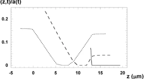
Figure 7. Resealing process. a) Porous poreless transition in stable membrane at different starting states, as. Upper curve: transmembrane voltage is 0.5V at t<0 and 0.0V at t>0; lower curve: transmembrane voltage is 0.45V at t<0 and 0.0V at t>0. b) Resealing process of metastable membrane both at different starting states, as a* (0) and
g. (1),
a as
t T and t0 ( 2/ )e /kT( , and are defined by Eqs.2,4). The dot-dash line represents the function
2 2
a ath with the respective ordinate at the right-hand side;ath 3 (Benz and Zimmermann17); g 0.001N/m,
s 10
a and r is the relaxation time of the annealing process.
1.1.3.5. Membrane Rupture
After applying supercritical field, the metastable membrane becomes unstable immediately. The beginning state is a0 0. The time course of the process can be determined by Eq.12. In Fig. 6b the rupture process is shown at different transmembrane voltages. The process is similar to the poreless porous transition, but the pore state further increases after the very fast increase in pore state, resulting in the rupture of the membrane.
1.1.3.5.1 Resealing Process
Upon switching off the supercritical field before the limit state of metastability,
*( 0 )
a U V , has been attained, the membrane becomes metastable again. By means of Eq.13 the time course of the relaxation process, a t t( / )0 has been calculated both at different starting states, as and at different g values (see Fig. 7b). The dot-dash line is the a t t2( / )0 ath2 function in the case of g 0.001N/m, as 10, ath 3. For a ath, no ions are conducted. The shape of this dot dashed curve is the same as that of the measured conductivity versus time curves during the resealing of oxidized cholesterol membranes17. Therefore, as is physically plausible, the ion conductance is proportional to
2 2
( / )0 th
a t t a . Using the relaxation time ( r 0.55 sec) of the experimental resealing process at 400C (Benz and Zimmermann17) and the calculated relaxation curve in Fig.
7b, one can determine the absolute time scale: t0 0.55 sec/ 0.0125 44 sec.
1.2. Phenomenological theory of low voltage electroporation
In common electroporators cells can be transfected with foreign genes by applying V
700
150 pulse on the cell suspension. Because of Joule heating, the cell survival rate is 10 20% in these elecroporators. In a recently developed electroporator, termed the low-voltage electroporator (LVEP), cells are partially embedded into the pores of a micropore filter. In LVEP cells can be transfected by applying 25V or less under normal physiological conditions, at room temperature. The large increase in current density in the filter pores, produced by the reduction of current shunt pathways around each embedded cell, amplifies a thousandfold the local electric field across the filter and results in high enough transmembrane voltage for cell electroporation. The Joule heat generated in the filter pore is fast dissipated toward the bulk solution on each side of the filter, and thus cell survival in the low-voltage electroporator is very high, above 98% while the transfection efficiency for embedded cells is above 90%. In this chapter the phenomenological theory of LVEP is developed. The transmembrane voltage is calculated along the membrane of the cell for three different cell geometries. The cell is either fully, partially or not embedded into the filter pore. By means of the calculated transmembrane voltage the distribution of electropores along the cell membrane is estimated. In agreement with the experimental results cells, partially embedded into the filter pore, can be electroporated by as low as 1.8 3.5V applied voltage. In the case of
V
25 applied voltage 90% of the cell surface can be electroporated if the cell penetrates further than half of the length of the filter pore.
1.2.1. Introduction
Biological membranes are known to become transiently more permeable by the action of short electric field pulses1 4 when the threshold value of the transmembrane voltage, about 0.5 1V , is exceeded. (The transmembrane voltage is defined by the potential difference between the inner and outer surfaces of the cell membrane.) This phenomenon is called electroporation or electropermeabilization and it can be used to transfect cells with foreign genes5. Electroporation of biological cells is commonly carried out in a cell suspension using parallel plate capacitor chamber6. The field between the plates is essentially homogeneous since the cell density is low. The voltage required for electroporation varies from 150V to 700V across a 0.2cm gap of physiologic solution ( 0.15MNaCl). The applied voltage depends on factors such as the spacing between the
capacitor plates, the cell type, and solution temperature. The field strengths needed for suspension electroporation normally vary between 750-2000 V/cm. The resulting current produced by these fields in the low resistivity physiologic solution is in the range of 25- 100A. Substantial Joule heating, electrode products, and solution electrolysis are byproducts produced by these fields in cell suspension7, and thus the cell survival rate is low. For COS-7 cells the survival rate in suspension experiments varies from 10%
(Ref.8) to 20% (Ref.9). These survival rates are in agreement with the rates quoted by commercial companies for their systems (Personal communications with BTX Corp., Life Technologies, Inc., and Savant/E-C Apparatus, Inc.)
Figure 1. Schematic of low-voltage electroporator (LVEP). Shaded areas mark the cylindrical carbon electrodes at the top and the bottom of the vertical chamber. The chamber is divided by a micropore filter. The plane of the filter aligned perpendicular to the symmetry axis of the cylindrical chamber is marked by a heavy solid line. The inset shows a magnified part of the filter with cells partially embedded into the micropores. Note that in the figure the chamber is stretched along its symmetry axis. In reality the chamber's inner length and diameter is 2 and 1 cm, respectively.
Recently, an alternative to cell suspension electroporation (SEP); the method of low- voltage electroporation (LVEP), was introduced10 16. The schematic of the low-voltage electroporator (LVEP) is shown in Fig.1 (reproduced from Ref.17). The vertical chamber consists of two mirror image halves. The inside diameter of the cylindrical chamber is
cm
1 , with cylindrical porous carbon electrodes enclosing the upper and lower ends of the chamber. The carbon electrodes apply the input signal, and are separated by 2cm. This produces a cylindrical measurement volume with dimension of 1cm in diameter and 2cm in length. A polycarbonate NucleporeTM filter (its plane aligned perpendicular to the symmetry axis of the chamber) is sealed into the center of the chamber, and the cells are then embedded into the filter pores (see enlargement in Fig.1) by using a hydrostatic pressure of 25 30mmHg. In LVEP as low as 2 25V applied voltage is sufficient to induce electroporation because 40% of the applied voltage drops in the 13 m long micropores of the filter17. The average field across the entire chamber for 10V input is less than 5V/cm, while the average field across the filter with cells is about 3000V/cm.
Thus the field in a LVEP is highly inhomogeneous, amplified about 1000 times in conjuntion with the increase in current density through the filter pores. However, the current produced in this system is only 25-50mA. The bulk temperature increase caused by a 90ms pulse of 10V is less than 0.003oC and the local Joule heating generated in the filter pore is dissipated in less than 0.3ms (Appendix 1). Because of the negligibly small Joule heating the cell survival rate is above 98% (Refs.12,16).
The development of the phenomenological theory of SEP started almost 40 years ago.
The transmembrane voltage around a spherical cell placed into a constant, subcritical electric field, V( ), was determined by solving the Laplace equation18,19. The field is subcritical as long as the absolute value of the transmembrane voltage is below the critical value, Vcr 0.5 1V. When the field is switched on at time t=0 the steady state transmembrane voltage, V( ), is attained after the charging of the membrane. In this case the solution can be separated to the steady state and transient part, f(t), as follows:
] )][1 ( [1.5
= )]
( )][
( [
= ) ,
( t V f t REocos e t/
V (1) where R is the radius of the cell, Eo is the field strength far from the cell, is the angle (azimuthal angle) between the direction of Eo and the vector directed from the center of the cell to the considered membrane segment, and is the membrane's charging time constant. According to Eq.1 the absolute value of V( ) is maximal at the poles of the cell, while it is zero at the equator.
In the case of supracritical fields, when electroporation takes place, however, there is no closed form solution of the Laplace equation. The azimuthal dependence of the transmembrane voltage, Vexp( ,t) was measured on a spherical sea urchin egg, stained with voltage sensitive fluorescence dye, at different time points after the application of supracritical electric field20 22. These measurements showed that: i) those regions of the cell membrane which would experience supracritical transmembrane voltage appear to be porated within less than 1 s, ii) the transmembrane voltage remains symmetric around the z-axis (the axis going through the poles of the egg), although it decreases significantly within a certain range around the pole.
We notice that the transmembrane voltage, V( ,t), can be calculated by means of Eq.1 not only at subcritical pulses but also at supracritical pulses if the cell membrane is assumed to be unporated. In reality pore formation takes place where the absolute value of this calculated transmembrane voltage exceeds the critical voltage, Vcr. In the case of supracritical electric pulses the phenomenological theory of SEP has been developed by Kinoshita and his co-workers. They assumed that the probability of pore formation is directly proportional to |V( ,t)| Vcr, where V( ,t) is defined by Eq.1. Thus, at any time t after the application of the supracritical pulse, the excess specific conductivity in the porated region of the membrane, m( ,t), is:
cr o
cr o
m cr
o
cr o
m
m V f t V
V t f t V
V t V
V t t V
t | ( )| ( )
) (
| ) ( ) | , (
| = ) , (
|
| ) , ( ) | , (
= ) ,
( (2)
where at = o, |V( )| assumes its global maximum. By using the above function for the excess membrane specific conductivity the Laplace equation was solved numerically by Hibino et al.21,22. The solution was in accordance with the measured transmembrane voltage, Vexp( ,t). At any given time, t, the excess specific conductivity of the membrane at the pole, m(0,t), was the only adjusted parameter of the theory of SEP.
The analysis of the experimental data revealed that m(0,t) gradually increased as long as the electric field was on. After switching off the field the decrease of m(0,t) could be described by two exponentials with time constants 7 s and 500 s. We note that the above theory is more complicated in the case of an asymmetric electroporation model22.
In this chapter, after defining the geometrical and material parameters of the system in the 1.2.2. Model section the solutions of the Laplace equation are presented in the 1.2.3 Results section for different lengths of cell penetration into the filter pore. In the 1.2.4.
Discussion section the calculated electric field is compared with the field around a single spherical cell in cell suspension and the importance of the current density amplification (CDA) is discussed. The distribution of the electropores along the membrane is calculated for different cell geometries. The calculated minimal applied voltage needed to induce electroporation is compared with the available experimental result and the efficiency of electroporation is defined and calculated for different cell geometries.
1.2.2. Model
1.2.2.1. Geometry of the Model of Low-Voltage Electroporator
The LVEP can be modelled by N electrically identical, parallel units, where N is the total number of the filter pores. One unit consists of a filter pore and its surrounding. The pore is cylindrical (pore length is 13 m and pore radius is 1 m) and its symmetry axis is perpendicular to the surface of the filter. The unit itself is assumed to be a cylinder too, its symmetry axis (z axis) coincides with the symmetry axis of the pore, while its cross sectional area, 254.5 m2/unit, is equal with the average filter area per filter pore.
Figure 2. The geometry of a unit of the low voltage electroporator. White area represents the filter, while gray area marks the bulk solution regions on both side of the filter and the filter pore. Solid line shows the cell membrane. (A) Cell is partially and (C) fully embedded into the filter pore. (D) Cell is out of the filter pore. (B) Transmission electron micrograph of human erythrocyte in the filter pore; the finger length is about
m 8 .
The cross section of a unit along the z axis is shown in Fig.2a. Grey area marks the filter pore and the bulk regions on both side of the filter, while white areas represent the filter around the pore. Solid line show the cell membrane. The vertical, z axis is the symmetry axis of the unit, while the horizontal axis measures the radial distance, r, from the symmetry axis. The unit contains one cell of surface area 137.3 m2, which is the average surface area of an erythrocyte23. In Fig.2a,c and d the cell is partially embedded, fully embedded into the filter pore, and outside the pore, respectively. In each case the center or symmetry axis of the cell coincides with the z axis of the unit. Outside the filter pore the cell is assumed to be spherical (Fig.2d). The geometry and location of the cell can be given by its radius (r2 =3.305 m) and the coordinate of its center, z2. When the cell is fully embedded into the filter pore its geometry is assumed to be two truncated spheres connected with a cylindrical tube (Fig.2c). In this case the geometry and location of the cell can be described by the center and radius of the lower truncated sphere (z1 and r1), the outer radius of the tube (rt =0.9 m) and the center and radius of the upper truncated sphere (z2 and r2). In the case of partially embedded cells the same parameters define the location and geometry of the cell with the restriction that one of the truncated spheres is a hemisphere (at the tip of the finger) of radius rt. The part of the cell which is penetrated into the filter pore is called the finger of the cell. The geometry of the cell partially and fully embedded into the filter pore has been confirmed by direct observation10,14,17 . Fig.2b