How can contemporary climate research help to understand epidemic dynamics? – Ensemble approach and snapshot attractors
T. Kovács1,a)
Institute of Theoretical Physics, Eötvös University, Pázmány P. s. 1A, H-1117 Budapest, Hungary.
(Dated: 13 August 2020)
Standard epidemic models based on compartmental differential equations are investigated under continuous parameter change as external forcing. We show that seasonal modulation of the contact parameter superimposed a monotonic decay needs a different description than that of the standard chaotic dynamics. The concept of snapshot attractors and their natural probability distribution has been adopted from the field of the latest climate-change-research to show the importance of transient effect and ensemble interpretation of disease spread. After presenting the extended bifurcation diagram of measles, the temporal change of the phase space structure is investigated. By defining statistical measures over the ensemble, we can interpret the internal variability of the epidemic as the onset of complex dynamics even for those values of contact parameter where regular behavior is expected. We argue that anomalous outbreaks of infectious class cannot die out until transient chaos is presented for various parameters. More important, that this fact becomes visible by using of ensemble approach rather than single trajectory representation. These findings are applicable generally in nonlinear dynamical systems such as standard epidemic models regardless of parameter values.
PACS numbers: SIR model, seasonal forcing, ensembles, snapshot attractor, transient chaos
I. BACKGROUND
The effort to estimate short and long-term behavior, system parameters, possible control strategies, and also social impact of COVID-19 pandemic stimulated an explosion of disease modelling1and scientifically demanding examinations from many different point of view made by various community members and research groups around the globe. Although the present situation is rather new, we have many examples from the history that helped to lay down basic mathematical rules of disease propagation. The celebrated SIR (suscepti- ble - infectious - recovered) model2splits the population into three disjoint parts and deals with the number of individuals in these sub-populations as time goes on.
The SIR model and its variants [SI, SIS, SEIR, SEIRS, RAS] show qualitatively similar dynamics and are in good agreement with observations. In a homogeneous environment these models possess a globally stable fixed point attractor as a disease equilibrium3. Omitting the stochastic nature of real world disease spread4–7, the deterministic SIR-like mod- els present diverse and reach dynamics. The non-linearity of the model8–11and also the time dependent internal forcing can be considered as a source of complexity.
Sufficiently large seasonal forcing or different mixing rates between sub-populations can cause large oscillations and also period doubling cascades12–18. It has also been demon- strated that for certain values of system parameters the non- autonomous models of recurrent epidemics (measles, mumps, rubella, H5N1 avian influenza) show chaotic behavior6,19–21. Traditional SIR-like epidemic models are dissipative nonlin- ear low-dimensional systems with constant, periodic, quasi- periodic22, or term-time3,23 external forcing whose dynamics
a)Electronic mail: tkovacs@general.elte.hu
is governed by (chaotic) attractors in phase space. Further- more, even if the long-term dynamics is regular and the final state of the system is a fixed-point attractor the route to this condition might be rather complex. Many studies examined the role of finite-time irregularity in ecological models24–27 as well as in epidemic dynamics9,23,28,29concluding the rele- vance of transient behavior.
It is known from dynamical systems theory that chaotic at- tractors always can be characterized by the natural measure corresponding to the distribution of possible states in phase space30–32. It turned out, however, that traditional numerical methods, such as monitoring a single chaotic long-term tra- jectory, fail in case of arbitrary forcing (like smoothly vary- ing parameters). Obviously, if one wants to model such a system (e.g. the changing climate with shifting atmospheric CO2 concentration), this shortcoming has to be overcome.
The mathematical concept of snapshot attractors33, known for many years in (theoretical and experimental) dynamical systems community34–41, fulfills entirely our wish.
Briefly, snapshot attractors are time-dependent objects in phase space of non-autonomous dynamical systems. Thus the shape of snapshot attractors is changing in time while their fractal dimension might even remain constant39. Furthermore, obtaining one single trajectory in a system with arbitrary driv- ing force, does not provide the same result as the ensemble approach (many trajectories emerging from slightly different initial conditions) in the same system at a given time instant.
This effect is the consequence of the fact that ergodicity is not satisfied as the system is driven aperiodically42. This con- clusion generated the recent opinion that the changing cli- mate should be scrutinized by ensemble approach (parallel climate realizations) rather than averaging a single long-term time series43–48.
In this work a seasonally forced deterministic epidemic model with monotonically changing contact rate (due to, for instance, vaccination or restricting the movement of the popu-
arXiv:2008.05205v1 [q-bio.PE] 12 Aug 2020
lation) is presented. We propose that the statement by Ref. 43
”climate change can be seen as the evolution of snapshot at- tractors”also holds for disease spread dynamics with contin- uously changing contact parameter.
In Section II the epidemic model is defined. After that, the results about stationary (Sec. III) and changing epidemic (Sec. IV) are presented. Section V is devoted to conclusions.
II. STANDARD EPIDEMIC MODEL
Compartmental disease models describe the number of in- dividuals in a population regarding their disease status: sus- ceptible (S), infectious (I), or recovered (R). Although, these models involve many simplifications (such as the progression of infection or difference in response of individuals) they per- formed well in real world epidemic situations49. There are two major groups of epidemic models: the SIR-like cluster that characterizes lifelong immunity (e.g. measles, whoop- ing cough), and the SIS-like class (containing mostly sexually transmitted diseases) which portrays repeated infections49.
Here we study the SEIR equations50 that involves a fourth group in addition to previous ones. More concretely, we as- sume that an individual enters the population at birth as sus- ceptible and leaves it by death. A susceptible becomes ex- posed (E) when contacting one or more persons, called infec- tive(s), that can transmit the disease. In an incubation period the exposed individuals are infectious but are not yet infec- tious. After this term they become infective and become later immune or recovered.
The mathematical model associated with above description reads as follows
dS
dt =m−bSI−mS, dE
dt =bSI−(m+a)E, dI
dt =aE−(m+g)I, dR
dt =gI−mR
(1)
with the following notations and assumptions51: (i)S,E,Iand Rare smooth functions of time and the size of the whole pop- ulation remains unchanged,S+E+I+R=1; (ii) there are equal birth and death rates (m); (iii) the probability that an exposed individual remains in this class for a time periodτ after the first contact is exp(−aτ),where 1/ais the mean (or characteristic) latent period; (iv) similarly 1/ggives the mean infectious period, the time period that an individual spends as infectious before recovery; (v) immunity is permanent and re- covered individuals do not re-enter to susceptible class. The contact rate b(t), the average number of susceptibles con- tacted per a single infective per unit time, is the origin of the spread of the disease. In the case of annual periodicity
b(t) =b0(t)[1+b1cos(2πt)]. (2) andtis measured in units of years.
When the system parameters are kept constant (m,a,g,b0,b1=0), the solution of Eq. (1) shows weakly dumping oscillation with a globally stable equilibrium (b>g). In this case the dynamics can be further characterized by the expected number of secondary cases caused by an infectious individual in the susceptible population. This is known as the basic reproductive ratio, and can be expressed denoted here by R0 =ba/[(m+a)(m+g)].13 R0 essen- tially determines whether a disease can (R0>1, endemic equilibrium) or cannot (R0<1, infection-free) persist in a population. Provided that latent and infectious periods are short, i.e.a,gm,one can use the approximationR0=b/g.
There are observations, for example in childhood diseases or avian influenza, that do not show damped characteristics rather (ir)regular cycles instead. This phenomenon can be linked to seasonal variation in contact rateb(t)or in recruit- ment rateg19. It has already been noticed that in case of peri- odic forcing,b0(t) =b0=const. in Eq. (2), chaos emerges in epidemic time series3,21,52. Similarly to the Lorentz84 model53 wherein the solar irradiation induces seasonal ef- fect, the SEIR model with variable contact rate is a non- autonomous low-order system with well-defined chaotic at- tractor in the phase space at certain parameter values. The low dimension of the phase space allows to visualize its pat- tern comfortably.
As a result of the fixed population size, point (i) above, one of the four equations (traditionally the equation forR) can be omitted. In addition, the infectious and exposed groups turn out to be linearly related to the first order13 at least, see Figure S1 in supplementary material. Consequently, the S−I phase portrait represents the state space texture accu- rately. Plotting one trajectory in theS−Iplane of the phase space one would observe a coil design due to the explicit time dependence of the model, b16=0. A conventional method to make a periodically forced systemautonomousis to take
”pictures” about the phase space with the same frequency as the excitation acts, i.e. making a stroboscopic map31,32. By choosing an initial timet0and purely sinusoidal force in Eq. 2 (b0(t) =const.) one can interpret the filamentary shape of the chaotic attractor by defining the stroboscopic mapt0 modT =0.Therefore, the periodic variation in Eq. (2) yields amannually stationary epidemicwith steady attractor.
Eq. (2) assumes a constant average contact rateb0.We have an annual period starting with its maximum at t =0.54 In physical or biological context this means the largest contact rate possibly due to school term, vacation and holidays, sea- sonal breeding pattern in a seabird colony, etc. Eq. (1) with the following parameters, corresponding to measles6, shows irregular dynamics:m=0.02 year−1,a=35.84 year−1,g= 100 year−1,b0=1800 year−1,b1=0.28 year−1. The above parameters lead toR0≈18.Numerical calculations show that for lower mean values of the contact rate periodic fixed-point attractors exist. For instance, biannual cycles atb0≈1500.
For more detailed asymptotic dynamics see the bifurcation di- agram in Figure 1 (blue curve).
Until nowb0was kept as a constant. Following the climate change methodology monotonic variation in b(t) through b0(t)is established. Equation (3) specifies the temporal de-
cay of the mean contact rate
b0(t) =
(1800 ift≤tst
1710e−α(t−tst)+90 ift>tst. (3) Heretst represents the time until the epidemic is stationary, i.e. b0=const., this is set to be 250 years after initialization.
This amount of time seems to be enough since the conver- gence of trajectories to the attractors is much shorter,tc≈50 years. The exponentαis the decay rate ofb0(t).In this study αtakes three values 0,04 yr−1,0.01 yr−1,and 0.004 yr−1,and b0always starts at 1800, i.e. from the chaotic regime. Eq. (3) implies that limt→∞b0(t) =90. This means that the critical value of mean contact rateb0=100 (or in terms of basic re- production rateR0≈1) is reached at different times aftertst, according toα.
The main motivation of this study is based on Eq. (3). Con- sidering, for example, the time series of childhood measles in London after World-War II (between 1945 and 1990), the vaccination program (starting in 1968) changed dramatically the number of cases3,28,55. Beside the medical treatment, if available, other artificially forced decline in contact rate (such as gradual lockdown prescribed by administration) can be im- itated by Eq. (3) resulting in a changing epidemic. This secu- lar variation of parameterb0gives a clear analogy to climate change models and the framework applied in this field.
III. STATIONARY EPIDEMIC A. Parameter dependence
The bifurcation diagram basically reveals the long-term dy- namics, excluded the initial transients, in a given parameter range. Classically, one single trajectory sampled by strobo- scopic map serves the blue shape of bifurcation diagram in Figure 1. In case of the stationary or stationary epidemic (b0=const.) complex dynamics arises for certain parame- ter values in the SEIR model,b0&1770. We should note, and it is going to be essential in our analysis, that the bifurcation diagram can also be established in a different way. That is, a large number of initial conditions are placed in the phase space and their evolution is monitored for sufficiently long time, but much shorter (one or two orders of magnitude) than that of the single trajectory considered above. Due to the er- godicity of the stationary chaotic dynamics the end-points of the ensemble members portray exactly the same pattern56.
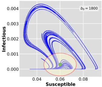
The same applies for the phase space pattern, too. Fig. 2 de- picts the chaotic attractor obtained afterT =2500yr integra- tion and 1600 initial conditions distributed uniformly in phase space. The same picture is obtained by one single trajectory after 200k year simulation. A representativeS−Iphase por- trait is pictured in Figure 2. The chaotic attractor (b0=1800) has been established fairly early and it remains unchanged when viewed after integer multiples ofT =1yr. Neverthe- less, choosing a different day of the year, the same applies eith a different pattern inS−Iplane.
FIG. 1. Bifurcation diagram of the SEIR model with stationaryb0. The variableSis plotted on the same year of the day starting att0=0.
The classical diagram (blue curve) is obtained by integrating 2000 initial conditions fort=15000yrs and the last 500 points stored.
For low parameter values cycles are determined by annual periodic- ity. There are many period doubling visible (shorter blue segments), however, the first one that routes to chaos starts atb0≈1250.The end-points of the same trajectories are plotted after 500yr iteration indicating long-lived transients (green). Clearly finite time chaotic motion unfolds the extra structure of bifurcation diagram. Upper x-axis evaluates the basic reproductive ratio derived from system pa- rameters.R0=1 is also marked (red arrow) to indicate the edge of endemic equilibrium. Long-term dynamics forR0<1 (b0<100) implies a dying out infection in population. The inset display real permanent chaos. Top box displays theR0of common diseases for comparison only. (Ebola∗: based on 2014 Ebola outbreak.)
Transient chaos, complex behavior on finite-time scales57, manifests before a trajectory comes to an attractor, both in dissipative as well as in conservative systems. In general, the attractor can be a simple object in the phase space, for in- stance, a fixed-point or a limit cycle. Following the time evo- lution of the ensemble before it approaches the attractor, one can capture other ingredients of the bifurcation diagram by considering the initial transients. To do this, the uniformly distributed 2000 trajectories are integrated for 500 years and the corresponding state space positions are stored. This fea- ture becomes visible in the green vague domain that extends along the blue curve. Clearly, transient chaos has a significant contribution to the dynamics forb0&125.
B. Ensemble view
The initial transients are usually thrown away in long-term dynamical analysis. However, the complexity might appear just in this phase of motion as indicated by the bifurcation diagram in Figure 1, already in the stationary case. Illus- trating the role of finite time chaotic behavior in the SEIR
FIG. 2. The stationary chaotic attractor in theS−I phase plane.
The ensemble is plotted at three different time instants: t = 500,1250,2500 years with perfect overlap. The green circle de- picts thehSi and hIi values from Fig. 3 (middle panel) while the ellipse indicates the associated standard deviations (bottom panel), respectively. Note that the green circle is a weighted average (a kind of ’barycentre’) of the trajectories along the attractor rather than its geometrical focus.
epidemic model we track the evolution of 1600 different ini- tial conditions distributed uniformly in a cubeS= [0.9999; 1], E= [0; 0.00005],I= [0; 0.00005],.
Fig. 3 demonstrates how the individual members of the ensemble reach the attractor at different time instants. For those values of contact parameter when the epidemic shows biannual (b0=1500) cycles one can observe clearly that the chaotic transients die out sooner or later (top panel). While in the case of permanent chaos (b0=1800) it is not so, since the irregular property is perpetual (middle panel).
Introducing classical statistical measures on the ensemble one can quantitatively keep track of transient effect. The mean hA(t)i=1/N∑Ni=1Ai(t)(where Ai(t)denotes an observable corresponding to theith member at time t) designates how fast the initial irregularity terminates and also adverts the average transient time. One can observe the similar characteristics for both thehSiandhIicurves, fixed-point and chaotic attractors (top and middle panels), respectively.
In the stationary epidemic model one might expect that after some time the extent of the attractor remains constant suggest- ing that all of the individual trajectories in the ensemble have reached it. The standard deviation,
σA= (hA2i − hAi2)1/2, (4) refers to the size of the attractor in the direction ofA.Figure 3 (bottom panel) depictsσSandσI in case ofb0=1800.The initial small values of standard deviations show that the en- semble moves together at the beginning of integration. Then, the members spread out in the phase space (≈30−50 years) and after a while start to approach the attractor. This time is longer for parametersb0=1500 (not shown) butσSis smaller.
FIG. 3. Ensemble view of stationary dynamics. Top and middle:
the mean ofS(blue) andI (red) variables vs. time. Some of the individual trajectories are also shown sampled by stroboscopic map (only theSco-ordinate). The individual trajectories arrives sooner or later the biannual fixed-point attractor (see for example the cyan parallel dots fort>230 in top panel). Bottom: standard deviations of the same variables as in the middle forb0=1800. The constant value of average and standard deviation after the convergence time demonstrates that the ensemble has reached the attractor and then spread along it.
Stationary epidemic with constantσAessentially means that after the transients the phase space structure does not change in time. This can be visualized by using of ensemble ap- proach. Without loss of generality we always start our sim- ulation att=0 (that corresponds to that part of the year with highest seasonal amplitude b(t)) and take the next picture about the ensemble att modT =0 that coincides the same day of the year.
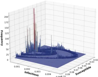
Thenatural distributionof a chaotic attractor31comes from the fact that the dots visit certain parts of the filamentary struc- ture more frequently than others. Moreover, this distribution is stationary and does not depend on initial conditions. Instead of investigating a 3D frequency diagram (see supplementary Figure S2), we plot the projectionI of trajectories wander- ing on the chaotic attractor in Figure 2. To obtain Figure 4, a fine grid is defined in theS−Iphase plane and the num- ber of points in each cell is plotted against the variableI.The histogram consists of four different ensembles. Ensemble 1,2,
FIG. 4. Natural distribution on the chaotic attractor (b0=1800) pro- jected onto theIvariable aftert=8500 years. The distribution does not depend on the individual members of the ensemble. The fre- quency has been cut at 3500 for the clarity.
and 3 covers the same volume in the phase space but involves slightly different initial state vectors. Ensemble 4 lays out ini- tial conditions from other part of phase space. The distribution clearly shows the same pattern for all four ensembles.
IV. EPIDEMIC CHANGE
In a changing epidemic the parameter(s) of the system is(are) varying as time goes on. One might think that, say, a decreasing of the contact parameterb0means to walk along the bifurcation diagram slowly from right to left, and terminat- ing at a safe destination withR0<1.In this section we will show that this idea is fairly naive due to the internal variability and the transient effects in the epidemic. To capture the dy- namics properly in this scenario, the ensemble approach and the concept of snapshot attractor is desirable.
A. Snapshot attractor geometry and natural distribution According to the common measles parameters we start the switch-off process, called also epidemic change, from the chaotic attractor (b0=1800) according to Eq. (3).
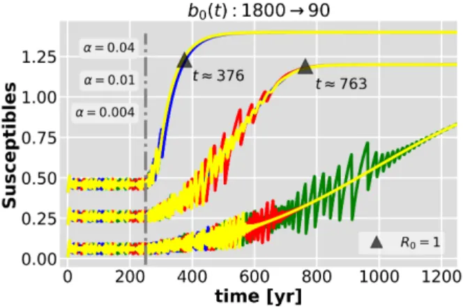
Recent studies56reveal that starting from the chaotic attrac- tor well after that the trajectories reached it, the evolution of different states might be rather diverse. That is, transient dy- namics becomes important again while the parameter change appears in the system. In Figure 5, four trajectories are se- lected from the chaotic attractor and their time dependence is followed. It can be immediately seen that different colors reach the fixed-point attractor at different times. For instance, in case ofα =0.004 (bottom curve), first the blue, then the yellow, red, and green curves arrive at the fixed-point attrac- tor. One can pick up other trajectories that will have longer or shorter oscillations. Furthermore, the previous order of colors, i.e. transient times, might change withα,as demon- strated by the middle curve. Therefore, we can point out, that it is worth investigating several trajectories simultaneously in- stead of following individuals. However, after the parameter shift is switched on, the shape of the chaotic attractor starts to
FIG. 5. Four trajectories plotted in blue, green, red, and yellow wan- dering on the chaotic attractor and their fate (inSvariable) after pa- rameter change sets in att=250 yrs (vertical line). The two scenar- iosα=0.01,0.04 are shifted by 0.2 units, respectively, for better visualization. The very peculiar time evolution of individual trajec- tories for differentαs suggests to use ensembles.
vary and forms a time-dependent set calledsnapshot attrac- tor. Thus, snapshot attractor is an object in the phase plane that contains the whole ensemble at a given time instant. We note that this mutation is not a result of the particular choice of initial phase (day of the year) of the mapping rather than the change of parameter. The geometrical alteration of the snapshot attractor is followed by the change of distribution on it. Nevertheless, its form and the distribution is independent of the choice of the ensemble and the onset (tst) of parameter decay.
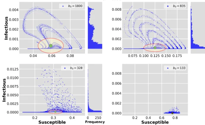
Figure 6 exhibits snapshot attractors drawn byN=104ini- tial conditions during the epidemic change. The mean contact rate decreases from top to bottom and left to right as speci- fied on each panel. Thus, every single plot corresponds to a different time instant of simulation. The top left panel, taken atT =219yr, coincides with the attractor in Figure 2 since the parameters of the system are the same fort<tst=250 yr. A more interesting aspect shows up on the following two panels. A filamentary structure, the fingerprint of chaotic be- havior, still dominates the pattern although the parameterb0 is well below of its original value (1800) as well as of 1770 where large extended chaotic attractors are formed in the bi- furcation diagram (Fig. 1 inset). In other words, for those con- tact rates (b0=835,328) no chaotic behavior is anticipated in the stationary dynamics.
Although, Figure 6 indicates the transmutation of the snap- shot attractor for decay exponentα =0.01 one can obtain similar alteration for different switch-off rates too. Slower scenario (e.g. α =0.004 in Eq. (3)) allows the attractor to keep its filamentary shape and maintain chaotic dynamics longer. From other perspective, the same parameter valueb0 is reached later whileα is smaller. The opposite is true for a faster parameter change, sayα=0.04.It can also be shown that approximately the same pattern belongs to the same con- tact value regardless the rate of change. That is, the faster the contact rate decay, the less pronounced the complexity in phase space.
FIG. 6. The evolution of the snapshot attractor with α =0.01. From left to right and top to bottom the ensemble is taken at t=219,333,447,618 yrs. The first picture still corresponds to stationary dynamics (beforetst=250 yr) with the original b0=1800.
Filamentary pattern persist for lowerb0values, too, where no stationary chaotic attractor exists in phase space according to the bifurcation diagram (Fig. 1). Still to be noted the physical extension of the snapshot attractor that is also time-dependent and their size varies significantly in both directions. Compare the scale of axes in different panels. The green circles and the red ellipses denote the same quantities as in Figure 2. Slim panels to the right of theS−Iphase planes display the natural distribution projected onto theIvariables. Forb0=133 most of the phase points accumulate around the fixed-point attractor (I≈10−3), therefore, no histogram is presented. Initial conditions cover the following state space volume:S= [0.9999; 1],E= [0; 0.00005],I= [0; 0.00005].
Other interesting feature is that although the contact rate b0decreases monotonically, the size of the snapshot attractors might increase, Figure 6 top right panel. This fact yields that the domain accessible by the dynamics can be larger. Thus the possible (S,I) pairs extend to larger domain in phase space even for smaller contact parameter. Furthermore, the average (green circles) and the standard deviation (red ellipses) also change in time. And this temporal behaviour cannot obtained from the classical view, only by using snapshot attractors.
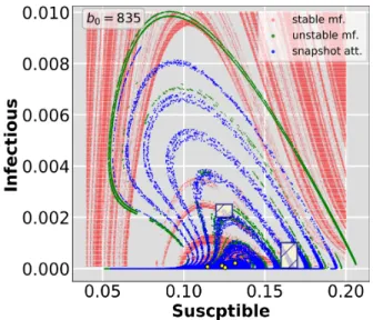
To understand this phenomenon we should recall the con- cept ofchaotic saddle. This non-attracting set with its sta- ble and unstable manifolds in phase space is responsible for the finite time chaotic behavior57. To construct the saddle numerically, we define two holes in the phase space (black rectangles in Figure 7). Then, a large number of initial con- ditions (N=3·105) are distributed uniformly in the region S= [0.04; 0.2],E= [0; 0.00005],I= [0.00001; 0.01]and the trajectories a integrated forT=30 years. Only those trajecto- ries are kept that do not enter the holes during the integration time. The initial conditions belonging to these trajectories draw the stable manifold of the saddle (red dots in Fig. 7), while those that are just before leave plot the unstable man- ifold (green dots.) The saddle itself is the intersection of its
manifolds, not shown here. The average lifetime of chaos (the inverse of escape rate,κ) can be estimated by calculating the time distribution of the non-escaped trajectories.
It is also known from the theory of transient chaos that the saddle’s manifolds have filamentary design just like the snap- shot attractors in Fig. 6. Analogously to chaotic attractor, sta- tionary dynamics with constant driving amplitude defines a stationary chaotic saddle related to certain parameter values of the system. Due to the continuous adjustment of the contact rate,b(t), in the changing epidemic model, the trajectrories do not have time to reach the attractor belonging to a givenb0 value. Consequently, a time dependent chaotic saddle is con- sidered, whose unstable manifold approximates the snapshot attractor56. This stationary saddle persist for very lowb0val- ues and its unstable manifold controls the finite time complex epidemic dynamics, Figure 7.
We emphasize at this point that the natural distribution as- sociated to the snapshot attractor also changes in time follow- ing the geometrical reorganization of the phase space pattern (histogram visualization in Fig. 6).
FIG. 7. The snapshot attractor (blue) and stable/unstable (red/green) manifolds of the stationary chaotic saddle at b0 =835. Discon- tinuities along the unstable manifold reflect to the escape condi- tions of the numerical scheme. The long-term dynamics of the sta- tionary model is visualized by the four tiny yellow circles around (S,I)≈(0.125,0.0004)as fixed-point attractors. The snapshot at- tractor coincides with the top right phase portrait in Figure 6
B. Parallel epidemic realizations
Similarly to climate research we can define the concept of parallel epidemic realizations. In standard disease models like Eq. (1) this can be done by using a large number of initial conditions as an ensemble in phase space and following their evolution as discussed in Section III A. This picture can be imagined as many copies of the epidemics obeying the same physical laws and being affected by the same time-dependent forcing48.
As we have seen before, in case of a changing epidemic, the time-dependent forcing has an impact on the natural mea- sure of the snapshot attractors. This fact results in a temporal change of the average values as well as internal variability.
To quantify the internal variability of the system (1) statisti- cal measures over the ensemble should be proposed like in the case of stationary epidemic. The variance or the standard deviationσAin Eq. (4) of the ensemble characterize the fluc- tuations around the averages indicating the inherent internal variability.
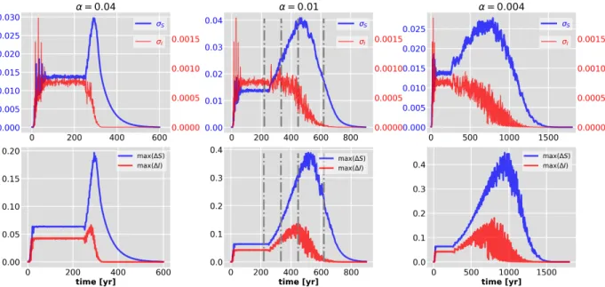
Top panels of Figure 8 show the ensemble standard devia- tionσS(blue) andσI for different decay ratesα.The paral- lel epidemic realizations contain 1600 numerically integrated trajectories sampled at integer multiplies of years. The con- vergence timetc,the time needed of the ensemble to reach and spread along the attractor, is found to betc=50yr. Both σS andσI are constant beforetst =250yr since till then the seasonal driving is constant, i.e. b0=1800yr−1.Right after this the contact rate starts to decrease (t>250yr) according to Eq. (3) both the mean state and the internal variability of the epidemic changes with time.
In changing epidemic, first, the graph of σS(t)increases,
after the maximum the trend follows nearlyb0(t),it decays to zero illustrating that the size of the attractor shrinks and asymptotically reaches the neighbourhood of a regular fixed- point attractor,(S,I) = (1,0),as expected forb0≈90 (R0= 0.9). The larger theα,the more regular, i.e less filamentary, the phase space geometry at the same time, see bottom panels in Fig. 8.
The shape of the standard deviation can be explained by transient chaos that occurs during the parameter change. The size of the green shaded band around the main feature in the bifurcation diagram (Fig. 1) already indicates that the size of the phase space region filled with transient chaos increases as b0reduces. To demonstrate this we call the attention to the horizontal dimension of the snapshot attractors in Figure 6.
The smoothly decreasing profile of the standard deviation af- ter reaching the maximum refers to the existence of transient effect up to very small parameter values.
Different maximum values of the σS(t)curves indicate a non-trivial relation between the internal variability and chang- ing rate ofb0.The largest value corresponds toα=0.01 (top middle panel), the other two scenarios (α =0.04 and 0.004) show roughly the same maximum size of the snapshot attrac- tor, albeit, at different time instants. Bottom panels present the maximal physical extension of the snapshot attractors versus time. These plots also supports our observations that the size of the attractor first increases and the shrinks to be a fixed- point attractor.
One possible explanation of this property is the relative
”coupling” between the timescales, that is, decay of forcing defined by the exponentαand the average lifetime of chaos in stationary dynamics at specific parameterb0.From a geomet- rical point of view, how close the snapshot attractor evolves to the unstable manifold of the stationary chaotic saddle at particular contact parameter. A detailed exploration of this feature is, however, postponed to a future study.
V. FINAL REMARKS
Parallel climate realizations, an effective and new frame- work in climate research, has been adopted to an epidemic model to explore the fading of the complexity due to the sys- tematic switch off the driving mechanism. The mathematical concept of snapshot attractors and their natural distribution demonstrates that single time series analysis is not capable to reflect the complex dynamics of a changing epidemic. In- stead of monitoring isolated events, the ensemble view of tra- jectories – parallel epidemic realizations – and its statistical description is desirable.
The temporal change of the attractor geometry and the dis- tribution on it reveals the internal variability of the dynamics.
The extension of the bifurcation diagram indicates the im- portance of transient chaos in the stationary dynamics as well as during the continuous parameter shift. No matter whether we start from a stationary state of the long-term dynamics, the switch-off process activates the hidden parts of the bifurca- tion diagram. Thus, the underlying non-attracting object, the chaotic saddle, or more precisely its unstable manifold, orga-
FIG. 8. Statistical measures of SEIR-ensembles. Top: The standard deviation of variableSandIfor various decay processes. The epidemic change starts attst=250 yrs well after the convergence time (tc≈50 yrs). Vertical dashed lines mark the time instants corresponding to phase space portraits in Figure 6. Bottom: The linear size of snapshot attractors in both variables indicate the role of transient chaos and internal variability of dynamics depending on the decay rateα.
nizes the system’s evolution.
The dissipative relaxation timescale, the inverse of the phase space contraction rate based on the divergence of the vector field of system (1), is extremely low,∼2−5 days, for measles. The other characteristic times are, the inverse of the switch-off rate and the escape rate from the chaotic saddle are, for comparison,α−1≈25−250 yrs,κ−1≈30−35 yrs, re- spectively. This latter is obtained a few particular contact rate.
This implies that the switching off process, with parameterα used in this study, is not quasistatic56. In other words, there is not enough time for trajectories to reach the stationary attrac- tor, either it is chaotic or regular, due to the nonstop parameter variation. Therefore, the dynamics of the switching off pro- cess shows much more complexity than that of the stationary scenario.
In the spirit of the investigated SIR-like classical epidemic model (1) with parameter shift58 of the contact rateb(t)we emphasize the importance of the finite time irregular dynam- ics. Our results reinforce the ”hidden” complex transients, and also the importance of time-dependent snapshot attractors not just for an epidemic with large reproductive ratio, such as measles and chickenpox, but for those with lower values
(R0&1) too.
The main conclusion of this study sheds light on the im- portance of the ensemble view and parallel realizations in epi- demic dynamics. Fig. 6 illustrates the general features one expects in the (long-term) prediction of any epidemics. Pre- dictions based on individual simulations are not reliable since, due to the chaotic nature of the dynamics, they can lead to many possible results, to any point of the snapshot attractor belonging to the time instant of the prediction. The ensemble approach is able to treat all possible outcomes as a whole, and predicts even the probability of the different permitted epi-
demic states. When convenient, statistical moments of this distribution can be determined, e.g. the average (providing the most typical epidemic outcome), or the variance (charac- terizing how broad the distribution of the permitted states is), but higher order moments might also be useful. Anyhow, one can thus follow how the statistical prediction changes in time.
ACKNOWLEDGMENTS
We benefited from useful discussions with T. Tél. This work was supported by the NKFIH Hungarian Grants K125171. The support of Bolyai Research Fellowship and ÚNKP-19-4 New National Excellence Program of Ministry for Innovation and Technology is also acknowledged.
1See the pre-filtered search on http://arxiv.org and https://connect.biorxiv.org/relate/content/181.
2W. . Kermack and A. G. McKendrick, “A contribution to the mathematical theory of epidemics,” Proceedings of the Royal Society A115, 700–721 (1927).
3M. J. Keeling, P. Rohani, and B. T. Grenfell, “Seasonally forced disease dynamics explored as switching between attractors,” Physica D Nonlinear Phenomena148, 317–335 (2001).
4H. C. Tuckwell and R. J. Williams, “Some properties of a simple stochastic epidemic model of sir type,” Mathematical Biosciences208, 76–97 (2007).
5L. J. S. Allen, “An introduction to stochastic epidemic models,” inMathe- matical Epidemiology, edited by F. Brauer, P. van den Driessche, and J. Wu (Springer Berlin Heidelberg, Berlin, Heidelberg, 2008) pp. 81–130.
6L. F. Olsen and W. M. Schaffer, “Chaos Versus Noisy Periodicity: Alterna- tive Hypotheses for Childhood Epidemics,” Science249, 499–504 (1990).
7P. J. Witbooi, “Stability of an SEIR epidemic model with independent stochastic perturbations,” Physica A Statistical Mechanics and its Appli- cations392, 4928–4936 (2013).
8L. F. Olsen, G. L. Truty, and W. M. Schaffer, “Oscillations and chaos in epidemics: a nonlinear dynamic study of six childhood diseases in copen- hagen, denmark,” Theor Popul Biol33, 344–370 (1988).
9D. A. Rand and H. B. Wilson, “Chaotic stochasticity: a ubiquitous source of unpredictability in epidemics,” Proceedings of the Royal Society B246, 179–184 (1991).
10B. M. Bolker and B. T. Grenfell, “Chaos and Biological Complexity in Measles Dynamics,” Proceedings of the Royal Society of London Series B 251, 75–81 (1993).
11M. J. Keeling and B. T. Grenfell, “Disease extinction and community size: Modeling the persistence of measles,” Science275, 65–67 (1997), https://science.sciencemag.org/content/275/5296/65.full.pdf.
12W. P. London and J. A. Yorke, “Recurrent outbreaks of measles, chicken- pox and mumps. i. seasonal variation in contact rates,” American Journal Epidemiology98, 453–468 (1973).
13J. L. Aron and I. B. Schwartz, “Seasonality and period-doubling bifurca- tions in an epidemic model,” Journal of Theoretical Biology110, 665 – 679 (1984).
14I. B. Schwartz, “Multiple stable recurrent outbreaks and predictability in seasonally forced nonlinear epidemic models,” J. Math. Biology21, 347–
361 (1985).
15R. M. Anderson and R. M. May,Infectious Diseases of Humans: Dynamics and Control(Oxford Science Publications, Oxford, 1992).
16S. Altizer, A. Dobson, P. Hosseini, P. Hudson, M. Pascual, and P. Rohani,
“Seasonality and the Dynamics of Infectious Diseases,” Ecology Letters9, 467–84 (2006).
17L. Stone, R. Olinky, and A. Huppert, “Seasonal dynamics of recurrent epidemics,” Nature446, 533–536 (2007).
18G. Rozhnova and A. Nunes, “Fluctuations and oscillations in a simple epi- demic model,” Physical Review E79, 041922 (2009), arXiv:0810.4683 [q- bio.PE].
19S. M. O’Regan, T. C. Kelly, A. Korobeinikov, M. J. O’Callaghan, A. V.
Pokrovskii, and D. Rachinskii, “Chaos in a seasonally perturbed SIR model: avian influenza in a seabird colony as a paradigm,” J Math Biol.
67, 293–327 (2013).
20P. G. Barrientos, J. A. Rodriguez, and A. Ruiz-Herrera, “Chaotic dynam- ics in the seasonally forced sir epidemic model,” Journal of mathematical biology75, 1655–1668 (2017).
21J. Duarte, C. Januaário, N. Martins, S. Rogovchenko, and Y. Rogovchenko,
“Chaos analysis and explicit series solutions to the seasonally forced sir epidemic model,” Journal of Mathematical Biology78, 2235–2258 (2019).
22S. Bilal, B. K. Singh, A. Prasad, and E. Michael, “Effects of quasiperiodic forcing in epidemic models,” Chaos26, 093115 (2016).
23I. Papst and D. J. D. Earn, “Invariant predictions of epidemic patterns from radically different forms of seasonal forcing,” Journal of the Royal Society Interface16(2019).
24A. Hastings and K. Higgins, “Persistence of Transients in Spatially Struc- tured Ecological Models,” Science263, 1133–1136 (1994).
25A. Hastings, “Transients: the key to long-term ecological understanding?”
Trends in Ecology and Evolution19, 39–45 (2004).
26B. K. Singh, P. E. Parham, and C.-K. Hu, “Structural Perturbations to Pop- ulation Skeletons: Transient Dynamics, Coexistence of Attractors and the Rarity of Chaos,” PLoS ONE6, e24200 (2011).
27A. Morozov, K. Abbott, K. Cuddington, T. Francis, G. Gellner, A. Hastings, Y.-C. Lai, S. Petrovskii, K. Scranton, and M. L. Zeeman, “Long transients in ecology: Theory and applications,” Physics of Life Reviews32, 1–40 (2020).
28D. J. D. Earn, P. Rohani, B. M. Bolker, and B. T. Grenfell, “A Simple Model for Complex Dynamical Transitions in Epidemics,” Science287, 667–670 (2000).
29K. Hempel and D. J. D. Earn, “A century of transitions in new york city’s measles dynamics,” Journal of The Royal Society Interface12, 20150024 (2015).
30J. P. Eckmann and D. Ruelle, “Ergodic theory of chaos and strange attrac- tors,” Reviews of Modern Physics57, 617–656 (1985).
31E. Ott,Chaos in dynamical systems, 2nd ed. (Cambridge University Press, Cambridge, 2002).
32M. Gruiz and T. Tél,Chaotic dynamics, 1st ed. (Cambridge University Press, Cambridge, 2006).
33For completeness, it should be mentioned that a generalization of snapshot attractors has been done and is referred to as pullback attractors in mathe- matical and climate research.59,60.
34F. J. Romeiras, C. Grebogi, and E. Ott, “Multifractal properties of snapshot
attractors of random maps,” Physical Review A41, 784–799 (1990).
35L. Arnold,Random dynamical systems, 1st ed. (Springer-Verlag, Berlin, Heidelberg, 1998).
36Y.-C. Lai, U. Feudel, and C. Grebogi, “Scaling behavior of transition to chaos in quasiperiodically driven dynamical systems,” Physical Review E 54, 6070–6073 (1996).
37J. Jacobs, E. Ott, T. Antonsen, and J. Yorke, “Modeling fractal entrainment sets of tracers advected by chaotic temporally irregular fluid flows using random maps,” Physica D Nonlinear Phenomena110, 1–17 (1997).
38Z. Neufeld and T. Tél, “Advection in chaotically time-dependent open flows,” Phys. Rev. E57, 2832–2842 (1998).
39G. Károlyi, T. Tél, A. P. de Moura, and C. Grebogi, “Reactive Particles in Random Flows,” Phys. Rev. Lett.92, 174101 (2004).
40J. C. Sommerer and E. Ott, “Particles floating on a moving fluid - A dynam- ically comprehensible physical fractal,” Science259, 335–339 (1993).
41M. Vincze, I. D. Borcia, and U. Harlander, “Temperature fluctuations in a changing climate: an ensemble-based experimental approach,” Scientific Reports7, 254 (2017), arXiv:1702.07048 [physics.flu-dyn].
42G. Drótos, T. Bódai, and T. Tél, “Quantifying nonergodicity in nonau- tonomous dissipative dynamical systems: An application to climate change,” Phys. Rev. E94, 022214 (2016).
43T. Bódai and T. Tél, “Annual variability in a conceptual climate model:
Snapshot attractors, hysteresis in extreme events, and climate sensitivity,”
Chaos22, 023110 (2012).
44J. D. Daron and D. A. Stainforth, “On predicting climate under climate change,” Environmental Research Letters8, 034021 (2013).
45G. Drótos, T. Bódai, and T. Tél, “Probabilistic Concepts in a Changing Climate: A Snapshot Attractor Picture*,” Journal of Climate28, 3275–3288 (2015).
46M. Herein, J. Márfy, G. Drótos, and T. Tél, “Probabilistic Concepts in Intermediate-Complexity Climate Models: A Snapshot Attractor Picture,”
Journal of Climate29, 259–272 (2016).
47S. Pierini, M. Ghil, and M. D. Chekroun, “Exploring the Pullback Attrac- tors of a Low-Order Quasigeostrophic Ocean Model: The Deterministic Case,” Journal of Climate29, 4185–4202 (2016).
48T. Tél, T. Bódai, G. Drótos, T. Haszpra, M. Herein, B. Kaszás, and M. Vincze, “The Theory of Parallel Climate Realizations,” Journal of Sta- tistical Physics (2019), 10.1007/s10955-019-02445-7.
49M. J. Keeling and T. D. Eames, “Networks and epidemic models,” Journal of the Royal Society, Interface2, 295–307 (2017).
50R. M. Anderson and R. M. May, “Directly Transmitted Infectious Diseases:
Control by Vaccination,” Science215, 1053–1060 (1982).
51D. L. In Epidemiology: SIMS 1974 Utah Conference Proceedings and S. K.L. Cooke (eds.), eds.,Transmission and control of arbovirus diseases (Philadelphia, 1975).
52G. Katriel and L. Stone, “Attack rates of seasonal epidemics,” Math Bio- science235, 56–65 (2012).
53E. N. Lorenz, “Irregularity: a fundamental property of the atmosphere,”
Tellus Series A36, 98 (1984).
54Choosing a different initial phase does not effect the qualitative picture of the dynamics. Only the shape of the phase space object differ to those ob- tained in present study.
55A. Becker, A. Wesolowski, O. Bjørnstad, and B. Grenfell, “Long-term dynamics of measles in london: Titrating the impact of wars, the 1918 pan- demic, and vaccination,” PLoS Comput Biol15, e1007305 (2019).
56B. Kaszás, U. Feudel, and T. Tél, “Death and revival of chaos,” Phys. Rev.
E94, 062221 (2016).
57Y.-C. Lai and T. Tél, Transient chaos /Lai-Tel. Berlin : Springer, c2011. 2011(Springer, 2011).
58Generally speaking, the time variability ofb0always results in a changing phase space structure according to the theory of snapshot attractors.
59M. Ghil, M. D. Chekroun, and E. Simonnet, “Climate dynamics and fluid mechanics: Natural variability and related uncertainties,” Physica D Non- linear Phenomena237, 2111–2126 (2008), arXiv:1006.2864 [math.DS].
60M. D. Chekroun, E. Simonnet, and M. Ghil, “Stochastic climate dynam- ics: Random attractors and time-dependent invariant measures,” Physica D Nonlinear Phenomena240, 1685–1700 (2011).
FIG. S1. Three dimensional chaotic attractor in the stationary SEIR model. The parameters are defined in the main text. It is striking that the infectious (I) and exposed (E) classes are approximately linearly related13(according to the ratiog/a). The relation is also indicated with red dashed line in theI−Esurface. Thus, one can investigate theS−Iprojection without loss of generality. This has been done in the present work.
FIG. S2. Natural distribution on the chaotic attractor of Fig. S1. A fine grid is defined in theS−Iplane and the number of phase points in each cell is recorded. The histogram shows that some part of the attractor are more frequently visited than others assigning the natural measure on it. Note that the height of the bars along theI≈0 axis is 1-2 order of magnitude larger than in the rest of the plot.
SUPPLEMENTARY MATERIAL
We present two illustrative plots related to the phase space structure of SEIR model (1) that complement the overall pic- ture of the paper but lack of the plots in the main text does not violates the understanding of the basic idea.