SimBPDD: Simulating differential distributions in Beta-Poisson models, in particular for single-cell RNA sequencing data

(1)

SimBPDD: Simulating differential distributions in Beta-Poisson models,

in particular for single-cell RNA sequencing data

Roman Schefzik

German Cancer Research Center (DKFZ), Heidelberg, Germany

Current affiliation: Medical Faculty Mannheim, Heidelberg University, Germany Roman.Schefzik@medma.uni-heidelberg.de

Submitted: December 19, 2020 Accepted: March 8, 2021 Published online: May 18, 2021

Abstract

Beta-Poisson (BP) models employ Poisson distributions, where the corresponding rate parameter itself is a Beta-distributed random variable. They have been shown to appropriately mimic gene expression distributions in the context of single-cell ribonucleic acid sequencing (scRNA-seq), a break- through technology allowing to sequence information from individual biological cells and facilitating fundamental insights into numerous fields of biology.

A prominent scRNA-seq data analysis task is to identify differences in gene expression distributions across two conditions. To validate new statistical approaches in this context, one typically has to rely on accurate simulations, as usually no ground truth for an assessment is available. We introduce several simulation procedures that allow to generate differential distributions (DDs) based on BP models. In particular, we describe how to create different types of DDs, mirroring various sources or origins of a difference, and different degrees of DDs, from a weak to a strong difference. The soundness of the simulation procedures is shown in a validation study in which theoretically expected model properties of the DD simulations are confirmed. The findings are in principle not restricted to the scRNA-seq context and may be gener- doi: https://doi.org/10.33039/ami.2021.03.003

url: https://ami.uni-eszterhazy.hu

283

(2)

ally applicable also to other application areas. The simulation approaches are implemented in the publicly available R packageSimBPDD.

Keywords:Beta-Poisson model, differential distributions, single-cell RNA sequencing, Wasserstein distance

AMS Subject Classification:62P10, 62-04, 62-08, 92-08

1. Introduction

Beta-Poisson (BP) models, sometimes also referred to as Poisson-Beta models, employ Poisson distributions, where the corresponding rate parameter itself is a Beta-distributed random variable [3, 4]. Thus, the BP distribution is an example of a mixed Poisson distribution [6] and a discrete compound distribution, respectively.

It is used in various theoretical and practical applications [8, 13, 15, 17].

Specifically, the BP distribution has been recently used in the biological context to model single-cell ribonucleic acid sequencing (scRNA-seq) data [15, 17]. Due to major technological advances, it is nowadays possible to sequence information from individual biological cells. Such single-cell sequencing, and in particular the scRNA-seq, enables the quantification of cellular heterogeneity and provides new fundamental insights into various biological fields [16], thus being highly relevant.

Along with the ever increasing amount of produced scRNA-seq data, there is a need to develop statistical methods for the analysis of such data [1]. The most striking difference compared to previous data obtained by bulk experiments is that gene expression in scRNA-seq data is available over multiple cells and not only as an average single point value. Consequently, models for scRNA-seq gene expression should take the form of distributions. Moreover, they should take account of the specific nature of scRNA-seq data (e.g. abundance of zero expression or increased variability). Besides other approaches, the BP distribution considered in this paper has been shown to model scRNA-seq data appropriately, where there are different procedures for model fitting and estimation of model parameters [2, 15].

To evaluate novel statistical methods in scRNA-seq data analysis, simulations play a very important role, as typically no ground truth is available for real data.

For instance, to adequately test and validate differential expression methods for scRNA-seq data [2], it is important to simulate differential distributions (DDs) in a reliable way. While there are already methods to do so [18], we here explicitly focus on a specific procedure to generate DDs in the scRNA-seq context using BP models. In particular, we describe how to create different types of DDs, mirroring various sources or origins of a difference, and different degrees of DDs, from a weak to a strong difference.

While the focus of this paper is on using BP models in the context of scRNA-seq data, the generation of DDs for the BP models is generally applicable also to other application areas, for both theoretical and practical considerations.

(3)

2. Beta-Poisson models in scRNA-seq data

We here consider Beta-Poisson (BP) models as introduced in [15], which have been found to appropriately mimic scRNA-seq data. Precisely, in [15], three different BP models are considered: a three-parameter BP model (BP3), a four-parameter BP model (BP4) and a five-parameter BP model (BP5).

The BP3 model is a mixture of Poisson distributionsPoi(𝜆1𝑢)with mean𝜆1𝑢, where 𝜆1 ∈ (0,∞) denotes a scaling parameter and 𝑢 ∼ Beta(𝛼, 𝛽) has a Beta distribution with parameters𝛼∈(0,∞)and𝛽∈(0,∞):

𝑋 ∼BP3(𝑥|𝛼, 𝛽, 𝜆1) := Poi(𝑥|𝜆1Beta(𝛼, 𝛽)).

Here, 𝛼 is a shape parameter, where a large 𝛼 indicates a high burst frequency (i.e. transcription rate, where transcription bursts correspond to an “on” state), and𝛽 is a scale parameter, with a large𝛽 indicating a high burst size [15, 17]. We can interpret this in the way that𝛼may reflect among others the number of zero expression values (i.e. the proportion of zero expression), while 𝛽 may mirror the size or magnitude of the non-zero expression values.

According to [15], the mean and the variance of the BP3model are given by E(𝑋) =𝜆1 𝛼

𝛼+𝛽 and

Var(𝑋) =𝜆1

𝛼

𝛼+𝛽 +𝜆²₁ 𝛼𝛽

(𝛼+𝛽)²(𝛼+𝛽+ 1), respectively.

As the BP3model can only account for count data (i.e. non-negative integers), the BP4 model is proposed in [15], which employs an additional parameter 𝜆2 ∈ (0,∞) to allow for modeling non-negative real-valued data, i.e., the usual data format we have to deal with after normalization of the raw scRNA-seq count data:

𝑌 ∼BP4(𝑥|𝛼, 𝛽, 𝜆1, 𝜆2) :=𝜆2BP3(𝑥|𝛼, 𝛽, 𝜆1).

In addition to what has been done in [15], straightforward calculations yield E(𝑌) =𝜆2𝜆1 𝛼

𝛼+𝛽 and

Var(𝑌) =𝜆²₂ (︂

𝜆1

𝛼

𝛼+𝛽 +𝜆²₁ 𝛼𝛽

(𝛼+𝛽)²(𝛼+𝛽+ 1) )︂

.

Finally, the BP5model has an additional parameter𝑝0∈[0,1]explicitly capturing the proportion of cells with zero expression (besides the parameter𝛼reflecting the burst frequency, as discussed before):

𝑍 ∼BP5(𝑥|𝛼, 𝛽, 𝜆1, 𝜆2, 𝑝0) :=𝑝01_{_𝑥=0_}+ (1−𝑝0) BP4(𝑥|𝛼, 𝛽, 𝜆1, 𝜆2)1_{_𝑥>0_},

(4)

with 1 denoting the indicator function. In addition to what has been outlined in [15], by applying corresponding formulas for mixture distributions, it can be computed that

E(𝑍) = (1−𝑝0)𝜆2𝜆1 𝛼 𝛼+𝛽 and

Var(𝑍) = (1−𝑝0)(E(𝑌)²+ Var(𝑌))−E(𝑍)².

Note that for𝜆2:= 1and𝑝0:= 0, the BP4and the BP5 models actually reduce to the BP3model.

3. Simulating differential distributions for Beta- Poisson models

The starting point of our procedure is a pre-processed (including quality control and normalization) real-experiment scRNA-seq data set in form of a (𝐺×𝐶) expression matrix, with𝐺denoting the number of genes and𝐶 the number of cells. We first fit a BP5 model to the expression data for each gene separately using the method provided by [15] in the R [12] package BPSC and obtain corresponding parameter estimates𝛼, 𝛽, 𝜆1, 𝜆2and𝑝0. Further, we test for each gene whether its distribution is indeed fitted well by the corresponding BP5model, using the procedure proposed in Section 3.2 in [15]. While filtering out low-quality fits, the cases (genes) that show a good fit, together with their corresponding parameter estimates, are kept in our pipeline and will be referred to as the controls in what follows.

We then simulate differential distributions (DDs) for each control𝑍 separately by manipulating the corresponding parameters 𝛼, 𝛽 and 𝜆1. We do not explicitly consider a manipulation of the parameter𝜆2here, as𝜆2only controls the transfor- mation from (a discrete spectrum of) non-negative integers (expression counts) to (a discrete spectrum of) non-negative real values (expression after normalization).

Moreover, we do not consider a manipulation of the parameter 𝑝0 at this point;

however, this will be discussed at the end of the section, when we explicitly describe how to construct differential proportions of zero expression (DPZ) in the context ofBP5 models.

Here, we consider multiplicative manipulations of the parameters𝛼, 𝛽 and 𝜆1

as follows, where we set 𝜆 := 𝜆1 for simplicity (as 𝜆2 is anyway not explicitly considered): 𝜆↦→∆𝜆𝜆,𝛼↦→∆𝛼𝛼,𝛽↦→∆𝛽𝛽. The parameters obtained by (one or multiple of) these transformations are then the corresponding parameters in the manipulatedBP5model𝑍. As˜ 𝜆∈(0,∞),𝛼∈(0,∞)and𝛽 ∈(0,∞), it must hold that ∆𝜆 ∈(0,∞),∆𝛼∈(0,∞)and ∆𝛽 ∈(0,∞), respectively, to get a reasonable model.

We not only want to create DDs, but also to incorporate different degrees 𝜃 of DD that range from weak to strong differences. Here, a degree𝜃 of DD between a control BP5 model𝑍 and a manipulatedBP5 model𝑍˜ is first introduced using a

(5)

multiplicative change (i.e., a fold change) with respect to the expected value:

E( ˜𝑍) =𝜃E(𝑍).

Inserting the corresponding expressions for the expected values and some algebra yields

𝜃= ∆𝜆·∆𝛼𝛼+ ∆𝛼𝛽

∆𝛼𝛼+ ∆𝛽𝛽. (3.1)

Hence,𝜃=𝜃(∆𝜆,∆𝛼,∆𝛽)can be viewed as a function of∆𝜆,∆𝛼and∆𝛽, and the degree of DD can be specified by varying∆𝜆,∆𝛼and∆𝛽, respectively. Vice versa, we may consider∆𝜆as a function of𝜃in case∆𝛼and∆𝛽are fixed, i.e.,∆𝜆= ∆𝜆(𝜃).

Analogously, ∆𝛼 = ∆𝛼(𝜃)in case∆𝜆 and∆𝛽 are fixed, and∆𝛽 = ∆𝛽(𝜃)in case

∆𝜆 and∆𝛼 are fixed. Note here again that𝜃 generally refers to the degree of the DD (weak to strong), while∆𝜆,∆𝛼or∆𝛽represents the model manipulation that is necessary in order to achieve a DD of degree𝜃.

To get an understanding of the influence of the single parameter manipulations and to facilitate interpretability, we here first only consider those cases in which only one of the three original BP5 model parameters is changed.

Case DLambda:

Here, the model is changed by manipulating the parameter𝜆only: 𝜆↦→∆𝜆𝜆, and

∆𝛼= ∆𝛽= 1.

By inserting the corresponding expressions in (3.1), we get 𝜃=𝜃(∆𝜆) =E( ˜𝑍)/E(𝑍) = ∆𝜆, i.e.,

∆𝜆= ∆𝜆(𝜃) =𝜃.

As 𝜃(0) = 0and𝜃(∆𝜆)→ ∞for∆𝜆 → ∞, 𝜃 is bounded from below by zero, but has no upper bound. Hence, the range for possible values of𝜃 is𝜃∈(0,∞). DDs of arbitrary degree can be created using either positively oriented or negatively oriented fold changes. Here, a negatively oriented fold change means thatE( ˜𝑍)<

E(𝑍), hence, 𝜃∈(0,1). Conversely, a positively oriented fold change means that E( ˜𝑍)>E(𝑍), hence,𝜃∈(1,∞). For instance, a positively oriented fold change of 3 in our setting here practically has the same effect as a negatively oriented fold change of 1/3, as we are only interested in the magnitude (i.e. the degree) of the difference here, and not in the direction of the change.

A manipulation of the scaling parameter 𝜆 in the BP model, while keeping Beta(𝛼, 𝛽) unmodified, changes location (mean) and size (variance). In contrast, the shape should be affected only to a minor extent by a manipulation as here, if at all [15, 17]. Moreover, a change of 𝜆 should not affect the proportion of zero expression too much.

(6)

Case DAlpha:

Here, the model is changed by manipulating the parameter𝛼only: 𝛼↦→∆𝛼𝛼, and

∆𝜆= ∆𝛽= 1.

By inserting the corresponding expressions in (3.1), we get 𝜃=𝜃(∆𝛼) =E( ˜𝑍)/E(𝑍) = ∆𝛼(𝛼+𝛽)

∆𝛼𝛼+𝛽 , i.e.,

∆𝛼= ∆𝛼(𝜃) = 𝛽𝜃 (𝛼+𝛽)−𝛼𝜃.

As𝜃(0) = 0andlimΔ𝛼→∞𝜃(∆𝛼) = 1+^𝛽_𝛼,𝜃is bounded from below by zero and has an upper bound1 +^𝛽_𝛼. Hence, the range for possible values of𝜃is𝜃∈(0,1 +^𝛽_𝛼).

DDs can be generated using positively oriented (i.e. 𝜃∈ (1,1 +^𝛽_𝛼)) or negatively oriented (i.e. 𝜃∈(0,1)) fold changes. However, DDs of arbitrary degree can thus be created using negatively oriented fold changes only.

Here, location, size and shape can change. Also, a manipulation of𝛼can affect the proportion of zero expression.

Case DBeta:

Here, the model is changed by manipulating the parameter𝛽 only: 𝛽 ↦→∆𝛽𝛽, and

∆𝜆= ∆𝛼= 1.

By inserting the corresponding expressions in (3.1), we get 𝜃=𝜃(∆𝛽) =E( ˜𝑍)/E(𝑍) = 𝛼+𝛽

𝛼+ ∆𝛽𝛽, i.e.,

∆𝛽= ∆𝛽(𝜃) =(𝛼+𝛽)−𝛼𝜃

𝛽𝜃 .

As𝜃(0) = 1 +^𝛽_𝛼 andlimΔ𝛽→∞𝜃(∆𝛽) = 0,𝜃is bounded from below by zero and has an upper bound1 +^𝛽_𝛼. Hence, the range for possible values of𝜃is𝜃∈(0,1 +^𝛽_𝛼).

DDs can be generated using positively oriented (i.e. 𝜃∈ (1,1 +^𝛽_𝛼)) or negatively oriented (i.e. 𝜃∈(0,1)) fold changes. However, DDs of arbitrary degree can thus be created using negatively oriented fold changes only.

Here, location, size and shape can change. However, a manipulation of𝛽should in principle not affect the proportion of zero expression too much.

We now consider a specific scenario, in which the expected value of the control BP5model is the same as that of the manipulatedBP5model. The construction of such a type of DD may be relevant in case one wants to check whether an scRNA- seq differential expression analysis method is able to detect differences that are not caused by differences with respect to means [7].

(7)

Case DAlphaBeta:

Here, the model is changed by manipulating both the parameters𝛼and𝛽 using a common parameter∆ := ∆𝛼= ∆𝛽: 𝛼↦→∆𝛼, 𝛽 ↦→∆𝛽, and ∆𝜆= 1.

As𝛼, 𝛽∈(0,∞), it must hold that ∆∈(0,∞)to get a reasonable model. As discussed before, the expected value of the manipulated model 𝑍˜ in this setting is the same as the expected value of the control model𝑍: E( ˜𝑍) =E(𝑍). We therefore introduce DDs by considering a multiplicative manipulation (i.e., a fold change)𝜃of the variance instead of the expected value, with somewhat more complex formulas involved:

Var( ˜𝑍) =𝜃 Var(𝑍).

Thus,

𝜃=𝜃(Δ) = Var( ˜𝑍)/Var(𝑍)

= 1

Var(𝑍) [︃

(1−𝑝0) (︃(︂

𝜆1𝜆2 𝛼 𝛼+𝛽

)︂2

+𝜆²2

(︂

𝜆1 𝛼 𝛼+𝛽+𝜆²1

𝛼𝛽

(𝛼+𝛽)²(Δ(𝛼+𝛽) + 1) )︂)︃

−(1−𝑝0)² (︂

𝜆1𝜆2

𝛼 𝛼+𝛽

)︂2]︃

= 1

Var(𝑍) [︂

(1−𝑝0) (︂

E(𝑌)²+𝜆2E(𝑌) + 𝜆1𝜆2𝛽E(𝑌) (𝛼+𝛽)(Δ(𝛼+𝛽) + 1)

)︂

−E(𝑍)² ]︂

, i.e., after some tedious calculations,

∆ = ∆(𝜃) = 1 𝛼+𝛽

⎛

⎝ 𝜆²₁𝜆²₂𝛼𝛽

(𝛼+𝛽)²(︁_{Var(𝑍)𝜃+}_E_(𝑍)2

1−𝑝0 −E(𝑌)²−𝜆²₂𝜆1 𝛼 𝛼+𝛽

)︁−1

⎞

⎠

= 1

𝛼+𝛽

⎛

⎝ 𝜆1𝜆2𝛽E(𝑌)

(𝛼+𝛽)(︁_{Var(𝑍)𝜃+}_E_(𝑍)2

1−𝑝0 −E(𝑌)²−𝜆2E(𝑌))︁−1

⎞

⎠.

For the degree of DD𝜃, we have the upper bound 𝐿up :=𝜃(0)

= 1

Var(𝑍) [︃

(1−𝑝0) (︃(︂

)︂2

+𝜆²₂ (︂

𝜆1 𝛼

𝛼+𝛽 +𝜆²₁ 𝛼𝛽 (𝛼+𝛽)²

)︂)︃

−(1−𝑝0)² (︂

)︂2]︃

= 1

Var(𝑍) [︂

E(𝑍) (︂

E(𝑌) +𝜆2

(︂

1 + 𝜆1𝛽 𝛼+𝛽

)︂

−E(𝑍) )︂]︂

and the lower bound 𝐿low:= lim

Δ→∞𝜃(∆)

(8)

= 1 Var(𝑍)

[︃

(1−𝑝0) (︃(︂

𝜆1𝜆2

𝛼 𝛼+𝛽

)︂2

+𝜆²₂𝜆1

𝛼 𝛼+𝛽

)︃

−(1−𝑝0)² (︂

𝜆1𝜆2

𝛼 𝛼+𝛽

)︂2]︃

= 1

Var(𝑍)[E(𝑍)(E(𝑌) +𝜆2−E(𝑍))].

Hence, the range for possible values of 𝜃is𝜃∈(𝐿low, 𝐿up), where0< 𝐿low<1<

𝐿up. It is therefore not possible to create arbitrary degrees of DD in each case, be it for positively or negatively oriented fold changes with respect to the variance.

Note again that here, only size and shape change, but not the location. However, also the proportion of zero expression can change, as 𝛼 varies, even though a variation of𝛽 should have no effect on this.

Finally, we consider the construction of manipulated BP5 models with an explicit difference with respect to the proportion of zero expression, compared to the control model.

Table 1. Settings for the DD simulations based on BP models, where5corresponds to “no” andXto “yes”.

Case DPZ:

Here, the model is changed by manipulating the parameter𝑝0 of the controlBP5

model only: 𝑝0 ↦→ 𝑝˜0 := 𝑝0 + ∆𝑝0, leading to differential proportions of zero expression (DPZ). While there is no intuitive feeling for the parameter ranges of the parameters𝜆, 𝛼and𝛽, which is the reason why we used the models described above to construct different degrees of DDs for the other cases, we have an immediate and clear interpretability of the parameter𝑝0.

As it has to hold that𝑝0+ ∆𝑝0 ∈[0,1](since𝑝0∈[0,1]), we choose∆𝑝0 as follows:

∆𝑝0=

{︃𝜃, 𝜃≤1−𝑝0,

−𝜃, 𝜃 < 𝑝0,

(9)

where 𝜃 ∈ (0,0.5]. A change of 𝑝0 should obviously affect the proportion of zero expression.

For an overview of all the considered settings described before, which are partly similar to those in [14], see the summaries in Tables 1 and 2. For the cases DLambda, DAlpha and DBeta, it is recommended to only consider negatively oriented fold changes𝜃(i.e.𝜃∈(0,1)), as all possible degrees of DDs can be achieved only using them. For the case DAlphaBeta, all possible degrees of DDs indeed can- not be achieved with negatively oriented fold changes, but neither this works for positively oriented fold changes. Hence, for reasons of consistency, we by default also focus on negatively oriented fold changes then.

Table 2. General overview of the different manipulated models 𝑍˜ of the control BP5 models 𝑍. Note that for the case DAl- phaBeta, 𝐿low := _Var(𝑍)¹ [E(𝑍)(E(𝑌) +𝜆2−E(𝑍))] and 𝐿up :=

1 Var(𝑍)

[︁E(𝑍)(︁

E(𝑌) +𝜆2

(︁

1 +_𝛼+𝛽^𝜆¹^𝛽)︁

−E(𝑍))︁]︁

. Here, Δmay refer to Δ𝜆,Δ𝛼,Δ𝛽 or Δ𝑝0, according to the descriptions of the corre-

sponding cases in the main text.

case manipulation choice of∆ possible values for𝜃

DLambda E( ˜𝑍) =𝜃E(𝑍) ∆ =𝜃 𝜃∈(0,∞)

DAlpha E( ˜𝑍) =𝜃E(𝑍) ∆ =_{(𝛼+𝛽)−𝛼𝜃}^𝛽𝜃 𝜃∈(0,1 +^𝛽_𝛼) DBeta E( ˜𝑍) =𝜃E(𝑍) ∆ =^{(𝛼+𝛽)−𝛼𝜃}_𝛽𝜃 𝜃∈(0,1 +^𝛽_𝛼) DAlphaBeta Var( ˜𝑍) =𝜃Var(𝑍) ∆ =_𝛼+𝛽¹ × 𝜃∈(𝐿_low, 𝐿_up)

(︃

𝜆1𝜆2𝛽E(𝑌) (𝛼+𝛽)(︁Var(𝑍)𝜃+E(𝑍)2

1−𝑝0 −E(𝑌)²−𝜆2E(𝑌))︁−1 )︃

DPZ 𝑝˜₀=𝑝₀+ ∆ ∆ =

{︂ 𝜃, 𝜃≤1−𝑝0

−𝜃, 𝜃 < 𝑝0 𝜃∈(0,0.5]

4. Validation study

4.1. Evaluation tools

To validate the soundness of our simulation procedures, we employ thewaddRtool available at https://github.com/goncalves-lab/waddR. Specifically, a semi- parametric, permutation-based test using the 2-Wasserstein distance is applied to compare two distributions𝐹𝐴 and𝐹𝐵 [10].

In our validation study, for each instance (here, each gene), information about 𝐹𝐴 (the control model) and 𝐹𝐵 (the manipulated model) is available in the form of a sample 𝑥𝐴,1, . . . , 𝑥𝐴,𝐶𝐴 from 𝐹𝐴, and 𝑥𝐵,1, . . . , 𝑥𝐵,𝐶𝐵 from 𝐹𝐵, respectively, where in general, 𝐶𝐴 does not need to equal 𝐶𝐵. In the context of scRNA-seq data, the sample sizes 𝐶𝐴 and 𝐶𝐵 correspond to the respective numbers of cells.

Using the corresponding empirical cumulative distribution functions𝐹ˆ𝐴 and𝐹ˆ𝐵as

(10)

approximations, the (squared) 2-Wasserstein distance𝑑is then computed by

𝑑( ˆ𝐹𝐴,𝐹ˆ𝐵)≈ 1 𝐾

∑︁𝐾 𝑘=1

(𝑄^𝛼_𝐴^𝑘−𝑄^𝛼_𝐵^𝑘)²

≈(ˆ𝜇𝐴−𝜇ˆ𝐵)²

⏟ ⏞

location

+ (ˆ𝜎𝐴−ˆ𝜎𝐵)²

⏟ ⏞

size

+ 2ˆ𝜎𝐴𝜎ˆ𝐵(1−𝜌ˆ𝐴,𝐵)

⏟ ⏞

shape

⏟ ⏞

variability

, (4.1)

with (𝑄^𝛼_𝐴^𝑘)𝑘=1,...,𝐾 and (𝑄^𝛼_𝐵^𝑘)𝑘=1,...,𝐾 denoting the 𝛼𝑘-quantiles of 𝐹ˆ𝐴 and 𝐹ˆ𝐵, respectively, where we use equidistant levels 𝛼𝑘 = ^𝑘⁻_𝐾^0.5, 𝑘 = 1, . . . , 𝐾. Here, ˆ

𝜇𝐴,𝜇ˆ𝐵 denote the corresponding empirical means, ˆ𝜎𝐴,ˆ𝜎𝐵 the corresponding empirical standard deviations, and

ˆ

𝜌𝐴,𝐵:= Cor((𝑄^𝛼_𝐴¹, . . . , 𝑄^𝛼_𝐴^𝐾),(𝑄^𝛼_𝐵¹, . . . , 𝑄^𝛼_𝐵^𝐾))

the sample Pearson correlation coefficient between(𝑄^𝛼_𝐴^𝑘)𝑘=1,...,𝐾and(𝑄^𝛼_𝐵^𝑘)𝑘=1,...,𝐾. For the calculations, we use𝐾:= 1000here.

For each instance separately, we calculate the corresponding 2-Wasserstein distance as a test statistic and obtain a p-value using a semi-parametric, permutation- based testing procedure involving a generalized Pareto distribution approximation to estimate very small p-values accurately. Along with the p-value, the decomposition of the 2-Wasserstein distance in (4.1) may help to judge whether overall differences between two distributions (i.e. BP models) are mainly due to differences with respect to location (referring to differences with respect to the expected values), size (referring to differences with respect to the standard deviations) and/or shape (referring to differences not mainly caused by differences with respect to expected values and/or standard deviations) [5, 9].

To explicitly test for DPZ, we use Fisher’s exact test, applied to each instance separately.

4.2. Setting

In the following validation study, we start with the real-experiment scRNA-seq data set in [11], downloaded fromhttps://hemberg-lab.github.io/scRNA.seq.

datasets/human/tissues. The data set consists of log2-transformed TPM (tran- scripts per million) expression values, normalized for both gene length and sequencing depth, for 301 cells, where we only keep those genes from the original data set that are expressed in at least three cells. A BP5model is fitted to each gene in the data set using the R package BPSC [15]. Specifically, maximum likelihood estimation combined with a binning approach to reduce computation time is employed to estimate the model parameters, using the standard R functionoptimfor optimization. For more details, in particular the choice of initial values for the BP model optimization, see Section 3 in [15]. To assess the quality of the BP5 model fits, a goodness-of-fit test statistic comparing the observed and expected frequencies

(11)

from the model is considered, where a Monte-Carlo method is used to generate a suitable null distribution that is employed to derive a corresponding p-value𝑃. A gene is then declared to be fitted well by the BP model if 𝑃 ≥0.05. For details, see Section 3.2 in [15]. In our study, 8773 genes are declared to be fitted well by the corresponding BP5 model. For the further analyses, we keep only these well- fitted genes as controls, from which manipulated BP5 models are then constructed according to the procedures discussed before. At this point, we emphasize that for our purposes here, the real data set in [11] is only used for obtaining reasonable BP model parameters in the scRNA-seq context, from which the control and manipulated BP models in our purely numerical experiments are constructed. However, no specific biological investigations or aspects are considered in our validation study.

For each case (see Tables 1 and 2), we here consider five different degrees 𝜃 of DD, ranging from weak to strong, where the explicit choices for 𝜃 are shown in Table 3. Note that for the cases DLambda, DAlpha, DBeta and DPZ, these degrees of DD can be achieved for all 8773 genes in the simulation study, and all these genes are used in the studies. In contrast, for the case DAlphaBeta, due to the existence of the lower bound 𝐿low, we only keep those genes for the study for which the corresponding degree of DD can be achieved.

As representatives of the corresponding control and manipulated BP5 models, for each gene, we draw a sample from each model. In this context, the samples from a BP distribution are independent random draws. Specifically, the function rBP from theBPSC package is used for drawing the samples from the BP distributions, which combines the classicalrpoisandrbetafunctions for randomly drawing from Poisson and Beta distributions, respectively, in R. In our study, we for convenience consider situations in which the sample size (i.e. the number of cells)𝐶:=𝐶𝐴=𝐶𝐵

in both conditions (control and manipulated) is equal and cover a range 𝐶 ∈ {25,50,75,100,500} of examples for small to large sample sizes.

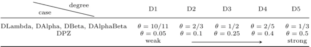
Table 3. Different degrees of DDs specifically chosen in the simulation study.

case degree D1 D2 D3 D4 D5

DLambda, DAlpha, DBeta, DAlphaBeta 𝜃= 10/11 𝜃= 2/3 𝜃= 1/2 𝜃= 2/5 𝜃= 1/3 DPZ 𝜃= 0.05 𝜃= 0.1 𝜃= 0.25 𝜃= 0.4 𝜃= 0.5

weak strong

4.3. Results

We now discuss the results for the validation study in terms of detection power and the decomposition of the 2-Wasserstein distance in thewaddRtest. In this context, for each fixed case, degree of DD and number of cells, detection power is defined as

detection power = # p-values≤𝛼

# tests (genes),

(12)

Table 4. Detection powers (in %), based on p-values at a 5%

significance level, with varying degrees of DD (D1: weak to D5:

strong), numbers of cells 𝐶∈ {25,50,75,100,500}and cases from Table 1.

case degree D1 D2 D3 D4 D5

DLambda waddRDD 1.39 8.48 21.86 32.06 38.31 Fisher DPZ 0.25 0.40 0.48 1.03 1.87 DAlpha waddRDD 1.57 7.67 18.03 26.73 32.73 Fisher DPZ 0.30 1.45 5.11 10.48 16.95 DBeta waddRDD 1.61 8.36 20.43 30.42 36.24 Fisher DPZ 0.25 0.42 0.96 1.74 2.74

𝐶=25

DAlphaBeta waddRDD 1.35 2.50 5.50 0.87 12.66 Fisher DPZ 0.20 1.64 7.55 16.53 25.67 DPZ waddRDD 1.37 2.09 23.50 54.21 65.61 Fisher DPZ 0.26 0.39 12.71 68.97 77.03 DLambda waddRDD 2.17 17.91 40.61 51.61 58.00 Fisher DPZ 0.40 0.52 1.58 3.21 5.49 DAlpha waddRDD 2.14 14.89 34.22 44.88 50.95 Fisher DPZ 0.59 3.65 14.97 29.02 38.32 DBeta waddRDD 2.47 16.77 37.25 48.93 55.08 Fisher DPZ 0.34 0.80 2.43 5.32 8.96

𝐶=50

𝐶=75

𝐶=100

𝐶=500

DAlphaBeta waddRDD 3.04 62.78 78.12 85.17 89.33 Fisher DPZ 2.87 59.94 92.03 96.65 98.57 DPZ waddRDD 23.74 70.61 87.99 91.51 93.25 Fisher DPZ 27.50 82.00 92.10 96.57 98.34

(13)

43.09%

50.75%

6.16%

44.97%

47.96%

7.07%

47.41%

44.54%

8.05%

50.1%

39.24%

10.66%

40.01%

47.65%

12.34%

D1 D2 D3 D4 D5

Degree of DD

C=25

DLambda

44.58%

37.01%

18.41%

46.03%

35.63%

18.33%

48.68%

32.48%

18.84%

49.5%

33.45%

17.05%

38.36%

48.4%

13.24%

D1 D2 D3 D4 D5

Degree of DD DAlpha

44.38%

46.77%

8.86%

45.94%

44.26%

9.8%

48.58%

40.4%

11.02%

50.23%

37.66%

12.11%

40.34%

46.15%

13.51%

D1 D2 D3 D4 D5

Degree of DD DBeta

21.72%

65.06%

13.23%

22.62%

65.21%

12.18%

26.1%

61.08%

12.82%

29.25%

60.04%

10.71%

36.78%

50.6%

12.62%

D1 D2 D3 D4 D5

Degree of DD DAlphaBeta

49.94%

21.6%

28.46%

41.49%

28.63%

29.88%

32.21%

44.64%

23.15%

36.14%

49.29%

14.57%

35.74%

52.22%

12.04%

D1 D2 D3 D4 D5

Degree of DD DPZ

shape size location

36.12%

57.99%

5.89%

37.81%

55.5%

6.69%

40.8%

50.97%

8.23%

45.92%

42.65%

11.43%

34.19%

49.97%

15.84%

D1 D2 D3 D4 D5

Degree of DD

C=50

DLambda

38.7%

37.32%

23.99%

40.68%

34.78%

24.54%

43.32%

32.1%

24.58%

47.16%

29.73%

23.11%

33.12%

49.5%

17.39%

D1 D2 D3 D4 D5

37.69%

52.43%

9.88%

39.5%

49.44%

11.06%

42.61%

44.54%

12.84%

46.3%

38.52%

15.18%

32.37%

51.6%

16.03%

D1 D2 D3 D4 D5

10.91%

63.45%

25.64%

12.06%

62.27%

25.67%

14.54%

60.75%

24.71%

20.8%

61.08%

18.11%

27.74%

59.08%

13.18%

D1 D2 D3 D4 D5

49.3%

18.93%

31.77%

41.21%

23.2%

35.6%

31.12%

31.28%

37.61%

22.16%

60.32%

17.52%

26.09%

57.53%

16.38%

D1 D2 D3 D4 D5

shape size location

32.19%

62.21%

5.6%

33.72%

59.89%

6.4%

36.42%

55.65%

7.93%

41.77%

46.4%

11.83%

30.91%

52.66%

16.43%

D1 D2 D3 D4 D5

Degree of DD

C=75

DLambda

35.34%

38.38%

26.27%

37.19%

35.72%

27.09%

40.31%

32.05%

27.64%

45.12%

28.57%

26.31%

32.25%

48.38%

19.37%

D1 D2 D3 D4 D5

33.86%

55.59%

10.55%

35.89%

52.31%

11.79%

38.83%

47.41%

13.76%

43.45%

39.96%

16.59%

33.49%

49.08%

17.43%

D1 D2 D3 D4 D5

6.5%

63.39%

30.11%

6.87%

60.15%

32.98%

9.05%

55.99%

34.96%

13.94%

55.56%

30.49%

23.27%

59.79%

16.94%

D1 D2 D3 D4 D5

49.17%

18.39%

32.44%

41.09%

22.05%

36.86%

31.12%

26.79%

42.09%

19.35%

53.78%

26.86%

22.15%

58.43%

19.42%

D1 D2 D3 D4 D5

shape size location

30.18%

64.37%

5.45%

31.45%

62.35%

6.2%

34.19%

58.06%

7.74%

39.66%

49.04%

11.31%

31.49%

48.3%

20.21%

D1 D2 D3 D4 D5

Degree of DD

C=100

DLambda

33.25%

38.99%

27.75%

35.28%

36.35%

28.37%

38.34%

32.5%

29.16%

43.3%

28.37%

28.33%

31.8%

44.3%

23.9%

D1 D2 D3 D4 D5

31.5%

57.65%

10.86%

33.65%

54.15%

12.19%

36.66%

49.22%

14.12%

41.64%

41.18%

17.18%

32.19%

47.61%

20.2%

D1 D2 D3 D4 D5

4.87%

63.11%

32.02%

5.53%

58.29%

36.18%

6.69%

52.61%

40.71%

10.81%

53.12%

36.07%

21.63%

58.06%

20.31%

D1 D2 D3 D4 D5

49.06%

17.87%

33.07%

41.17%

21.39%

37.44%

31.26%

24.89%

43.84%

19.15%

46.22%

34.63%

18.55%

59.77%

21.68%

D1 D2 D3 D4 D5

shape size location

25.02%

70.86%

4.12%

25.32%

70.05%

4.63%

25.9%

68.29%

5.81%

29.02%

61.61%

9.37%

33.94%

37.22%

28.84%

D1 D2 D3 D4 D5

Degree of DD

C=500

DLambda

27.71%

39.45%

32.84%

28.57%

37.44%

34%

29.84%

34.85%

35.31%

34.22%

29.05%

36.72%

35.58%

25.54%

38.88%

D1 D2 D3 D4 D5

26.41%

62.36%

11.23%

26.95%

60.27%

12.78%

28.25%

56.62%

15.13%

32.23%

48.42%

19.35%

35.29%

31.63%

33.07%

D1 D2 D3 D4 D5

0.9%

62.42%

36.68%

1.05%

59.02%

39.93%

1.49%

53.64%

44.88%

2.38%

42.77%

54.85%

15.3%

48.86%

35.84%

D1 D2 D3 D4 D5

48.06%

18.19%

33.76%

41%

20.99%

38.01%

32.4%

22.62%

44.98%

22.72%

21.96%

55.32%

15.16%

31.82%

53.02%

D1 D2 D3 D4 D5

shape size location

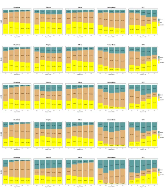
Figure 1: Decomposition results for the waddR test for the xed number of cellsC= 25, based on averages over those of the runs that are considered to show signicant DDs in that the corresponding p-value is less than or equal to 0.05, with cases according to Table ??.

1

Figure 1. Decomposition results for the waddR test for varying degrees of DD (D1: weak to D5: strong) and numbers of cells𝐶∈ {25,50,75,100,500}, based on averages over those of the runs that are considered to show significant DDs in that the corresponding

p-value is≤0.05, with cases according to Table 1.

with 𝛼∈ (0,1). Detection powers for the different numbers of cells for the standard level of 𝛼 = 5% are listed in Table 4. In general, for all cases, detection powers meaningfully increase with increasing numbers of cells. Moreover, they increase with increasing strength of the difference between the distributions (weak to strong degree of DD; D1 to D5). While only very little detection power can be

(14)

observed for the very weak degree of DD D1, the detection powers get bigger for the stronger degrees of DD, for which the differences become more and more obvious.

This intuitively makes sense and confirms in particular that the implementation of the varying degrees of DD from weak to strong in our simulation procedure is valid. When comparing the p-values of the waddR test and the separate DPZ test, we observe that DPZ can mainly be detected when the parameters 𝛼or 𝑝0

are changed (i.e. in the cases DAlpha, DAlphaBeta and DPZ). In contrast, DPZ typically plays only a minor role when the parameters 𝜆or 𝛽 are changed (i.e. in the cases DLambda and DBeta). This is in line with the theoretical properties and the interpretation of the parameters of the BP model.

A further confirmation that the simulation procedures are able to reflect what is to be expected from the underlying theory (Table 1) of the BP model is given by the decomposition of the 2-Wasserstein distance into location, size and shape parts within the waddR test. For the different degrees of DDs and numbers of cells, Figure 1 shows for all cases the average fractions of the location, size and shape parts with respect to the overall 2-Wasserstein distance for the waddR test based on those runs with a p-value less than or equal to5%. Again, the respective decomposition patterns meaningfully become more and more obvious the larger the number of cells is and the stronger the degree of DD is. In particular, the shape and location component in the cases DLambda and DAlphaBeta, respectively, are minor to negligible compared to the corresponding other components, in line with the theoretical models according to Table 1. Moreover, for instance, the shape component is more pronounced in cases in which the shape parameter𝛼is changed (i.e. in the cases DAlpha and DAlphaBeta) than in those where𝛼is not changed (i.e. in the cases DLambda and DBeta). An explicit change of the proportion of zero expression by manipulating the parameter 𝑝0 (case DPZ) can obviously also affect the shape.

5. Discussion

We have discussed how to create DDs of varying degrees, ranging from weak to strong differences, for BP models, using various manipulations of the BP model parameters. The soundness of our approaches has been shown in a validation study, in which theoretically expected properties of our procedures have been confirmed.

In particular, based on the construction of our simulations and their validation in the study, we can provide some guidance on how to generate DDs between two BP models when the difference shall be of a specific type. For instance, when no difference with respect to shape is desired, the DLambda simulation, in which only the BP model parameter𝜆is changed, can be used. Similarly, in case no difference with respect to location is desired, one can employ the DAlphaBeta simulation, in which the BP model parameters𝛼and𝛽are changed using a common manipulation parameter. In case there shall be no DPZ, one may rely on the DLambda or DBeta simulations, in which only the BP model parameters 𝜆 and 𝛽, respectively, are changed.

(15)

Despite the focus of this paper is on the application field of scRNA-seq data, the introduced procedures can in principle be applied also to settings in other research areas.

While we have presented first attempts to simulate DDs for BP models here, we by far did not consider all possible combinations of BP parameter manipulations.

This provides opportunities for future work, in which in particular interactions of changes when multiple BP parameters are manipulated simultaneously could be investigated in more detail. Moreover, up to now, only univariate BP distributions, that allow for individual (gene-wise) modeling, have been considered in the models here. However, certain variables may be correlated (such as genes in the scRNA- seq context), and taking account of specific correlation structures is an important issue that could be addressed in future extensions of the models.

Software availability. The simulations of DDs based on BP models presented in this paper are implemented in the R package SimBPDD, which is publicly available at https://github.com/RomanSchefzik/SimBPDD, along with documentation of the functions.

Acknowledgements. Angela Goncalves and Marc Schwering are thanked for helpful discussions and useful comments. Moreover, thanks are given to two anony- mous reviewers for valuable comments and suggestions. The work was funded by project VH-NG-1010 of the HGF.

References

[1] R. Bacher,C. Kendziorski:Design and computational analysis of single-cell RNA-sequencing experiments, Genome Biology 17 (2016), art. 63,

doi:https://doi.org/10.1186/s13059-016-0927-y.

[2] M. Delmans,M. Hemberg:Discrete distributional differential expression (D³E) – a tool for gene expression analysis of single-cell RNA-seq data, BMC Bioinformatics 17 (2016), art. 110,

doi:https://doi.org/10.1186/s12859-016-0944-6.

[3] J. Gurland:A generalized class of contagious distributions, Biometrics 14 (1958), pp. 229–

249,doi:https://doi.org/10.2307/2527787.

[4] M. S. Holla,S. K. Bhattacharya:On a discrete compound distribution, Annals of the Institute of Statistical Mathematics 17 (1965), pp. 377–384,

doi:https://doi.org/10.1007/BF02868181.

[5] A. Irpino,R. Verde:Basic statistics for distributional symbolic variables: a new metric- based approach, Advances in Data Analysis and Classification 9 (2015), pp. 143–175, doi:https://doi.org/10.1007/s11634-014-0176-4.

[6] D. Karlis,E. Xekalaki:Mixed Poisson distributions, International Statistical Review 73 (2005), pp. 35–58.

[7] K. D. Korthauer,L.-F. Chu,M. A. Newton,Y. Li,J. Thomson,R. Stewart,C.

Kendziorski:A statistical approach for identifying differential distributions in single-cell RNA-seq experiments, Genome Biology 17 (2016), art. 222,

doi:https://doi.org/10.1186/s13059-016-1077-y.

(16)

[8] K. L. Leask,L. M. Haines:The beta-Poisson distribution in Wadley’s problem, Commu- nications in Statistics–Theory and Methods 43 (2014), pp. 4962–4971,

doi:https://doi.org/10.1080/03610926.2012.744047.

[9] Y. Matsui,M. Mizuta,S. Ito,S. Miyano,T. Shimamura:D³M: detection of differential distributions of methylation levels, Bioinformatics 32 (2016), pp. 2248–2255,

doi:https://doi.org/10.1093/bioinformatics/btw138.

[10] V. M. Panaretos,Y. Zemel:Statistical aspects of Wasserstein distances, Annual Review of Statistics and Its Application 6 (2019), pp. 405–431,

doi:https://doi.org/10.1146/annurev-statistics-030718-104938.

[11] A. A. Pollen,T. J. Nowakowski,J. Shuga,X. Wang,A. A. Leyrat,J. H. Lui,N. Li, L. Szpankowski,B. Fowler,P. Chen,N. Ramalingam,G. Sun,M. Thu,M. Norris,R.

Lebofsky,D. Toppani,D. W. Kemp II,M. Wong,B. Clerkson,B. N. Jones,S. Wu, L. Knutsson,B. Alvarado,J. Wang,L. S. Weaver,A. P. May,R. C. Jones,M. A.

Unger,A. R. Kriegstein,J. A. A. West:Low-coverage single-cell mRNA sequencing reveals cellular heterogeneity and activated signaling pathways in developing cerebral cortex, Nature Biotechnology 32 (2014), pp. 1053–1058,

doi:https://doi.org/10.1038/nbt.2967.

[12] R Core Team:R: A Language and Environment for Statistical Computing, R Foundation for Statistical Computing, Vienna, Austria, 2020,

url:https://www.R-project.org/.

[13] J. M. Sarabia,E. Gómez-Déniz:Multivariate Poisson-Beta distributions with applications, Communications in Statistics–Theory and Methods 40 (2011), pp. 1093–1108, doi:https://doi.org/10.1080/03610920903537269.

[14] M. Schwering:Batch effects in single cell RNA sequencing analysis, MA thesis, Heidelberg University, 2017.

[15] T. N. Vu,Q. F. Wills,K. R. Kalari,N. Niu,L. Wang,M. Rantalainen,Y. Paw- itan:Beta-Poisson model for single-cell RNA seq data analyses, Bioinformatics 32 (2016), pp. 2128–2135,

doi:https://doi.org/10.1093/bioinformatics/btw202.

[16] Y. Wang,N. E. Nevin:Advances and applications of single-cell sequencing technologies, Molecular Cell 58 (2015), pp. 598–609,

doi:https://doi.org/10.1016/j.molcel.2015.05.005.

[17] Q. F. Wills,K. J. Livak,A. J. Tipping,T. Enver,A. J. Goldson,D. W. Sexton,C.

Holmes:Single-cell gene expression analysis reveals genetic associations masked in whole- tissue experiments, Nature Biotechnology 31 (2013), pp. 748–752,

doi:https://doi.org/10.1038/nbt.2642.

[18] L. Zappia,B. Phipson,A. Oshlack:Splatter: simulation of single-cell RNA sequencing data, Genome Biology 18 (2017), art. 174,

doi:https://doi.org/10.1186/s13059-017-1305-0.