Powerful calibration strategy for the two-layer viscoplastic model

(1)

Polymer Testing 99 (2021) 107206

Available online 23 April 2021

Powerful calibration strategy for the two-layer viscoplastic model

Attila Kossa

^*

, Andr ´ as Levente Horv ath ´

Department of Applied Mechanics, Faculty of Mechanical Engineering, Budapest University of Technology and Economics, H-1111 Budapest, Muegyetem rkp. 5., Hungary

A R T I C L E I N F O Keywords:

Viscoplasticity Viscoelasticity Parameter-fitting Stress integration scheme

A B S T R A C T

An efficient numerical integration scheme is proposed for the uniaxial loading of the two-layer viscoplastic (TLVP) model, which is a built-in material model in the commercial finite element software Abaqus. The particular version of the TLVP model under investigation is governed by linear isotropic plastic hardening rule with time-hardening nonlinear creep law. The new integration scheme can be easily implemented in any programming environment leading to a fast and robust tool to obtain the stress response in uniaxial loading for a given input strain history. The accuracy of the proposed algorithm is demonstrated and validated by comparing the results obtained with it to those calculated by Abaqus. A new calibration software with a graphical user interface is developed, which can fit the material parameters to the experimental data with arbitrary strain history in a uniaxial loading case. The new software is freely available to download from the webpage of the authors, and it is free to use for research purposes. The excellent performance of the new program is demonstrated by fitting the material parameters to three distinct experimental data sets.

1. Introduction

Constitutive modelling of polymer materials usually involves elas- ticity, plasticity and creep in the formulation of the mechanical behavior. There are many more additional features that can also be considered, but from the mechanical point of view, the above three pillars are the essential ingredients when we develop a constitutive model. It is important to emphasize that polymer materials often un- dergo finite deformations during applications. Therefore the finite strain formulation has to be adopted from continuum mechanics. The classical linearized theory of deformation can be used only for simple problems, where both the strains and displacement are small, therefore the difference between the reference and deformed configuration can be neglected. We can use numerous theories and models to characterize the elastic, plastic, and creep behaviors of materials. There exist elementary models to describe the creep behavior, but highly non-linear models are also available. Furthermore, we have several strategies (series connection, parallel connection, mixed connection) how to combine the elastic, plastic (or permanent), and creep behaviors in the formulation of the constitutive equation. The researchers continuously propose novel spe- cific models to characterize the mechanical behavior of their materials under investigation. This implies that we have an increasing number of viscoelastic-viscoplastic models available in the literature. These models are usually self-coded, and they are not available in commercial finite

element software. We have no general uniform model we can use for any kind of materials showing viscoelastic-viscoplastic characteristics.

However, it would be beneficial for the users in the industrial and research areas if they could use a non-linear viscoelastic-viscoplastic model, which is available in a commercial finite element software. The two-layer viscoplastic model (TLVP) available in Abaqus is an excellent candidate for this purpose [1]. The model consists of an elastic-plastic network that is in parallel with an elastic-viscous network. Any of the available creep models in Abaqus/Standard can be used for the dashpot element located in the elastic-viscous network. Furthermore, isotropic, kinematic, and even mixed non-linear plastic hardening rules can be specified for the elastic-plastic branch. Consequently, the TLVP model can be considered as a model class in which we can specify the actual behavior of the viscous and plastic elements.

The two-layer viscoplastic model proposed by Kichenin was origi- nally developed for polyethylene materials [2,3]. However, the model is also used to predict material responses of other materials than polyethylene. Kang et al. combined the TLVP model with indentation tests in order to obtain the material properties of the investigated materials (high nickel–chromium material and P91 steel) [4]. Figiel and Günther used the model to characterize the mechanical behavior of a metal matrix composite (SiC/Ti-6242) [5]. It is important to note they also investigated the model accuracy at elevated temperatures as well. They have found that the model is able to describe the material behavior at

* Corresponding author.

E-mail addresses: kossa@mm.bme.hu (A. Kossa), levente.horvath@mm.bme.hu (A.L. Horv´ath).

Contents lists available at ScienceDirect

Polymer Testing

journal homepage: http://www.elsevier.com/locate/polytest

https://doi.org/10.1016/j.polymertesting.2021.107206

Received 17 December 2020; Received in revised form 26 March 2021; Accepted 18 April 2021

(2)

different temperatures and strain rates. Charkaluk et al. performed 3D thermomechanical finite element simulations on cast-iron exhaust manifolds using the two-layer viscoplastic model in addition to the unified viscoplastic model [6]. Leen et al. have chosen the temperature-dependent TLVP model with a combined hardening rule for the material modelling of a high nickel-chromium material (XN40F) [7].

Their conclusion is the applied model provides excellent agreement with the cyclic stress-strain data of the material across a range of temperatures; additionally, it successfully captured the effect of different strain-rate values. Saber et al. presented a numerical study using the TLVP model to demonstrate the impact of crack location on creep crack growth in a P91 weldment [8]. Their particular model utilizes Norton’s creep law. Furthermore, they combined the material model with a damage model in order to predict the failure in the specimens. Farragher et al. employed the TLVP model in transient finite element calculations in order to predict the stress-strain-temperature cycles and the associated strain-rates for P91 steel used for high temperature, steam-pressurized pipes [9]. Their results revealed that the model can describe the combined cyclic elastic-plastic and creep deformations involving non-linear kinematic hardening/softening. In a latter work, the authors used the TLVP material model to characterize the mechanical behavior of the same material governed by non-linear isotropic softening [10]. The modified version of the two-layer viscoplastic model proposed by An et al. employs a strain-rate dependent plastic contribution in the constitutive equation [11]. The modified model is used to predict the mechanical behavior of ABS material. The modified formulation was adopted by Doh et al. for a modified polyphenylene oxide (MPPO) material [12]. Adel et al. used the TLVP model to characterize the mechanical behavior of a poly-methyl methacrylate (PMMA) material at a wide range of temperatures below glass transition [13]. They have found the TLVP model provided better agreement with the experimental data compared to the elasto-plastic material model they also investigated. Solasi et al. performed a series of uniaxial tensile tests on a perfluorosulfonic acid (PFSA) membrane material for different hydrations at room temperature [14]. They used the TLVP model to simulate the material behavior and they have found that the model performs very well in predicting the overstresses and relaxation times at different hydrations for different strain-rates. In addition, they underline a major advantage of the two-layer viscoplastic model, namely, it is available in Abaqus and there is no need to develop a user material subroutine. A recent paper demonstrates the applicability of the TLVP model in predicting the mechanical response of a microcellular polyethylene-terephthalate foam material at a wide range of temperatures [15]. The new results are based on the authors’ earlier work [16].

The authors performed a detailed analysis of the sensitivity of the parameters on the final results. In addition, they also investigated the performance of different optimization strategies in the parameter-fitting procedure. The calibrated parameters they found were used in an axisymmetric analysis of a thermoforming punch test to predict the variation of the thickness in the specimen [17]. In another recent study, the uniaxial behavior of small length-scale bone samples is reproduced using the TLVP model [18]. The paper concludes the model can repro- duce the stress response of single trabeculae subjected to uniaxial cyclic loading.

The calibration procedure for the parameters of the TLVP model is not a straightforward task. The resulting constitutive equation is highly non-linear even in uniaxial loading case and closed-form solutions for the time-strain-stress relations do not exist. A possible solution to fit the material parameters is to use a third-party optimization package, which involves Abaqus to calculate the stress response at every iteration step of the parameter fitting procedure. This task can be accomplished using Dassualt Systemes Isight software [19] for instance. The application of the software in parameter fitting of the TLVP model is demonstrated in Ref. [15] or in Ref. [13] for example. The main drawback of this method is the optimization is relatively slow as Abaqus has to be used for the calculations. A complete finite element calculation has to be performed

even when we use only one single element to simulate the uniaxial behavior. This paper aims to overcome this problem by presenting a robust numerical integration scheme to calculate the stress response, in uniaxial loading cases, of the TLVP model with linear isotropic hardening and time-hardening creep law. In addition, a freely available calibration software is developed with a graphical user interface to fit the material parameters. A major advantage of the parameter fitting approach compared to the series of experiments described by Abaqus, is the ability to obtain the material parameters from a single measurement.

Increasing the number of measurements will improve the accuracy of this method as well. However, in some cases the availability of the material samples can be limited. In these cases the parameter fitting approach is especially useful.

This paper is organized as follows. Section 2 presents the particular form of the TLVP model under investigation. The constitutive relations of the components are also presented in this section. The numerical integration scheme is summarized in Section 3, where the main contribution is the implicit midpoint integration scheme applied on the elastic-viscous network. Section 4 demonstrates the proposed scheme’s accuracy and performance by comparing the results with those obtained using the Abaqus built-in material model. The Python implementation of the calibration software is summarized in Section 5. Section 6 demonstrates the excellent performance of our new calibration software.

Parameter-fitting of the material constants is presented for three different loading cases with three different materials.

2. Two-layer viscoplastic model 2.1. Introduction

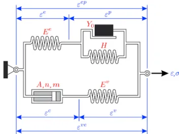
The one-dimensional schematic of the particular two-layer viscoplastic model under investigation is depicted in Fig. 1. The upper branch represents a classical elastic-plastic material model with linear hardening, whereas the lower branch is a Maxwell-type viscoelastic model with a non-linear dashpot component. The two networks are connected in parallel manner. The constitutive parameters associated with the members are visualized in the figure. In addition, the particular strain values are also shown. Upper index “” refers to the elastic-plastic network, whereas upper index “ve” corresponds to the viscoelastic branch.

The total stress and strain of the model are related to the stresses and strains in each network as follows:

σ=σ^ve+σ^ep, ε=ε^ve=ε^ep. (1)

Furthermore, the stresses and strains in each network can be

Fig. 1. One-dimensional idealization of the TLVP model.

(3)

decomposed based on the series-type connections as

σêp=σê=σ^p, εêp=εê+ε^p, (2)

σ^ve=σ^c=σ^v,ε^ve=ε^c+ε^v. (3)

It is noted here that the elastic component in the viscoelastic network is labeled with upper index „v” in order to distinguish it from the elastic member present in the elastic-plastic branch.

2.2. Constitutive relations

The constitutive equation of the model is derived for the strain- driven case, where the strain history ε(t)is given as input, and we are interested in the resulting stress response σ(t). This type of representation is more useful for parameter fitting strategies as the experimental tests usually performed using displacement-controlled setups. The following sub-sections present the constitutive equations for each network.

2.2.1. Elastic-plastic branch

The constitutive relation for the one-dimensional elastic-plastic solid with linear isotropic hardening governed by associative flow rule and Mises yield criterion is discussed in many textbooks [20,21]. The mechanical behavior of the elastic component is characterized by the Hooke’s law:

σê=Eêεê→ε˙ê= 1

E^eσ˙^e, (4)

where E is the corresponding Young’s modulus. The yield function of the plastic component is expressed as

F(σ^p,Y) = |σ^p| − Y, (5)

where Y denotes the current yield stress of the material. The yield criterion is formulated as:

F<0 →ε˙^p=0,F=0 →

{ε˙^p=0 elasticloading

ε˙^p∕=0 elastic− plasticloading (6) The evolutionary equation for the yield stress in the case of linear isotropic hardening can be written in the following form:

Y=Y0+Hγ, (7)

where Y0 denotes the initial yield stress value. The internal variable γ is calculated as the integral of the absolute value of the plastic strain-rate;

thus it can be considered as the accumulated plastic strain:

γ=

∫^t

0

|˙ε^p|dt→γ˙= |˙ε^p| (8)

The associative plastic flow rule in the one-dimensional case has the form:

ε˙^p=γ⋅sgn[˙ σ^p]. (9)

Imposing the consistency condition F˙ =0, one can eliminate γ ˙and the relation for elastic-plastic loading can be easily derived. Whether the strain input yields elastic or elastic-plastic loading, we can summarize the overall constitutive behavior as

σ˙^ep=

⎧

⎨

⎩

E^eε˙ elasticloading E^eH

E^e+Hε˙ elastic− plasticloading (10) The resulting differential equation can be reduced to an algebraic equation, thus a closed-form solution can be easily obtained even for plastic loading. However, this statement is not valid for 3D case [22].

2.2.2. Viscoelastic branch

The constitutive relation for the elastic component in the viscoelastic branch is simply expressed using the Hooke’s law. However, in order to distinguish the Young’s modulus associated with this element from the other one located in the elastic-plastic branch, we use the index ˝v˝to denote the elastic modulus of this component. Therefore, the stress and the strain-rate acting on this element can be written as

σ^v=E^vε^v→ε˙^v= 1

E^vσ˙^v. (11)

The creep component is modelled with the time-hardening creep law. It is important to note that other non-linear creep models are available in Abaqus, but the time-hardening law is an excellent candidate to model the non-linear creep characteristics. The general formula (valid for positive and negative stresses) for the strain-rate acting on this component is written as

ε˙^c=A⋅sgn[σ^c]⋅|σ^c|ⁿ⋅t^m, (12) where the sign and absolute value functions are needed because parameter n is generally non-integer. Three parameters are associated with the creep component, namely A, n and m.

The overall strain-rate can express the overall mechanical behavior of the viscoelastic branch:

ε˙^ve=ε˙^v+ε˙^c= 1

E^vσ˙^v+A⋅sgn[σ^c]⋅|σ^c|ⁿ⋅t^m. (13) Rearranging the terms, one can obtain the expression for the stress- rate as

σ˙^ve=E^vε˙− E^v⋅A⋅sgn[σ^ve]⋅|σ^ve|ⁿ⋅t^m. (14) Closed-form solution for σ^ve(ε(t))does not exist even not for linear strain path due to the highly nonlinear nature of the second term in the differential equation.

2.2.3. Overall constitutive equation

The overall one-dimensional constitutive model of the two-layer viscoplastic model under investigation for strain-driven case is simply obtained by summing the constitutive relations (14) and (10). Closed- from solution for the resulting differential equation cannot be obtained due to the highly non-linear nature of the viscoelastic component.

However, the two branches can be treated separately as the input strain history is the same for both networks due to the parallel connection.

Consequently, one can find the solution for the elastic-plastic part using the analytical solution, whereas the solution for the viscoelastic part can be obtained using a numerical integration scheme. The total stress in the model is obtained by adding the stresses in the two networks.

The Mises yield criterion used in the three-dimensional representation of the model is a pressure-independent yield criterion. This can be considered as a limitation in cases where the yield stress of the material shows significant pressure-dependency. There exist yield criteria (Drucker-Prager’s yield criterion, for instance), including the pressure part of the stress in the definition of the yield function, but the current version of the two-layer viscoplastic model implemented in Abaqus al- lows us to use the classical Mises-type yield criterion or the anisotropic Hill’s criterion.

2.2.4. Formulations in finite strain theory

The formulations above were derived in small-strain theory utilizing the engineering strain measure. But the constitutive equations can be extended to finite strain theory as well. To distinguish the true (or log- arithmic) and engineering (or nominal) strains we adopt the following notations is the followings: The engineering strain will be denoted by e, whereas the true strain will be ε. The relations between these measures are

ε=ln(e+1), e=exp[ε] − 1, (15)

(4)

whereas the rates are expressed by ε˙= e˙

1+e,e˙=exp[ε]⋅ε˙. (16)

If we use the true strain in constitutive relations (14) and (10), then the resulting stress will be the Cauchy stress in finite strain theory. In finite strain problems, the engineering stress (or nominal stress) will be denoted by P.

3. Numerical integration scheme

Our goal in the numerical integration scheme is to derive an approximate solution in discretized form for the constitutive equation.

In this analysis the engineering strain is given as input and we are seeking the resulting stress (either engineering or true) solution.

Subscript n indicates the particular value of a quantity at the beginning of the increment, whereas subscript n+1 refers to its value at the end of the increment. Subscript n+1/2 denotes the value in the middle of the increment. The time increment and the time value in the middle of the increment are

Δt=tn+1− tn,tn+1/2=tn+1+tn

2 . (17)

Since the variation of the engineering strain through the increment is considered to be linear, its expression can be written as

e(t) =en+e(t˙ − tn) (18)

with the engineering strain-rate definition e˙=Δe

Δt=en+1− en

Δt =e˙n=e˙n+1=e˙n+1/2. (19)

In finite strain case, the true strain-rate in the middle of the increment can be expressed using (16) as

ε˙n+1/2= e˙ 1+en+1/2

= Δe/Δt 1+en+1/2

. (20)

3.1. Elastic-plastic branch

For the discretized solution of the elastic-plastic network, the standard radial return algorithm is utilized. Since it is a widely used algorithm, only the final expressions are summarized below, more details can be found is textbooks [20,21].

First, the trial state is calculated:

σêp_trial=σêp_n +Eê⋅Δε. (21)

Then, the trial yield function is determined as

Ftrial=F(σ^ep_trial,Yn) = |σ^ep_trial| − Yn. (22)

Depending on the value of Ftrial two scenarios are possible. If Ftrial≤0, then the increment does not involve plastic deformation and therefore, the entire behavior is pure elastic. It follows that the stress and the yield stress at the end of the increment are simply obtained as

σ^ep_n+1=σ^ep_trial,Yn+1=Yn. (23)

In contrast, if Ftrial>0 then plastic deformation occurs. The increment of the plastic multiplier is calculated as Δγ= Ftrial/ (E+ H), whereas the stress and yield stress solutions at the end of the increment are expressed as:

σêp_n+1=σêp_trial− EêΔγ⋅sgn[σêp_trial],Yn+1=Yn+HΔγ. (24) It is noted here, the implicit integration scheme adopted for the elastic-plastic network is unconditionally stable.

3.2. Viscoelastic branch

For the numerical solution of (14) the implicit midpoint integration is used. Therefore the resulting algebraic equation becomes

σ^ve_n+1− σ^ve_n

Δt =E^vε˙n+1/2− E^v⋅A⋅sgn

[σ^ve_n+1+σ^ve_n 2

]

⋅

⃒⃒

⃒⃒σ^ve_n+1+σ^ve_n 2

⃒⃒

n

⋅t^m_n+1/2 (25)

In order to simplify the presentation here, we introduce the new notation x =σ^ve_n+1/2. The equation above then can be rearranged to have the form

R(x) =a+b⋅sgn[x]⋅|x|ⁿ− x (26)

with the following constants:

a=σ^ve_n +1

2ΔtE^vε˙n+1/2,b= − 1

2ΔtE^vAt_n+1/2^m . (27)

During the numerical solution, the equation R(x) =0 has to be solved. Since a closed-form solution does not exist, a local Newton- Raphson iteration can be applied to find x. The corresponding deriva- tive needed during the iteration is expressed as

R^′(x) =dR

dx= − 1+bn|x|ⁿ⁻¹. (28)

Once x=σ^ve_n+1/2is obtained one can easily determine the stress at the end of the increment as σ^ve_n+1=2σ^ve_n+1/2− σ^ve_n. The implicit midpoint integration scheme used for the viscoelastic network is also unconditionally stable.

4. Validation of the proposed algorithm

The stress results obtained by the numerical algorithm presented above were compared to those calculated using Abaqus for different loading cases involving wide ranges for the parameters and wide range for the strain-rate. It was found that the presented numerical scheme yields the same results for all test examples we investigated. However, it is important to emphasize two major differences:

a) The computational speed of the proposed algorithm is much higher (with several orders) than the corresponding Abaqus calculation.

b) The new numerical scheme is stable. The Abaqus calculations were terminated frequently if the step increment size was too large or if the viscoelastic strain error tolerance (parameter cetol in the input file) was not properly defined.

The first remark can be explained by the fact that for the Abaqus results, a complete finite element problem has to be solved using one single finite element. It requires additional computation resources. For problems involving creep Abaqus determines the suitable integration scheme. It uses either an explicit or an implicit integration scheme or switches from explicit to implicit in the same step as described in the theory manual. However, in a VISCO step needed to solve the corresponding problem, we can choose between the following two options:

explicit/implicit or explicit. For automatic increment size control in the step module, we can specify the value of the viscoelastic strain error tolerance (parameter cetol in the input file) which is needed for Abaqus to determine when to switch to the backward difference operator instead of using an explicit scheme. Using the fixed time increment setting, we do not have this option, and the software certainly employs the implicit scheme. We have found the simulations were terminated frequently for fixed time increments. Switching to automatic time increment helps to avoid this convergence issue, however, if the viscoelastic strain error tolerance is not properly selected, we face another convergence issue.

In order to demonstrate the phenomena described above, we present the results for one particular uniaxial loading history, which consists of linear segments defined by the following time – engineering strain

(5)

values: {{0,0},{2,1},{10,1},{16, − 0.2},{50, − 0.2}}. The loading history is visualized in Fig. 2.

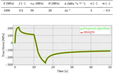
The material parameters used for the comparison are listed in Table 1. These are artificially chosen values, however, they are in the range which might correspond to the real materials.

It is important to note Abaqus requires parameters E>0 and 0<f<

1, which are related to elastic moduli in the networks as

E^v=f⋅E, E^e= (1− f)E, E=E^e+E^v. (29) Note E represents the instantaneous elastic modulus (obtained using

“infintite” strain-rate loading), whereas the long-term elastic modulus (obtained using “zero” strain-rate loading) equals to E^e. The numerical results using the proposed algorithm were obtained using a Wolfram Mathematica notebook. The code used for the calculation is provided in the Appendix. The Abaqus calculation was performed using one single eight-node linear brick element. Since the prescribed deformation is homogeneous in the element, reduced integration is used. Hybrid formulation is adopted as the Poisson’s ratio was set to 0.5 in the analysis. The boundary conditions were defined according to the strain history above. The input file and the description of the model are provided in the Appendix.

The maximum time increment was set to 0.1 s. Therefore at least 500 data points are calculated during the computations. It is essential to emphasize the proposed algorithm was stable in the entire domain, however using fixed time increment in Abaqus always led to convergence issues even at the beginning of the calculation. Therefore, automatic increment control had to be used to let Abaqus reduce the increment size from 0.1 to a smaller value. The calculated stress values are reported in Fig. 3 and Fig. 4, where the former one shows the results along the time, while the second Figure is a plot in the true strain – true stress coordinate system.

One can conclude the excellent agreement between the two calculations, which indicates the proposed scheme can be used to determine the stress values. The viscoelastic strain error tolerance was 10⁻⁶in the calculation above.

We investigated the effect of the value of the viscoelastic strain error tolerance in the Abaqus results. The detailed analysis is provided in the Appendix.

For the parameter-fitting procedure, it is required to reduce the corresponding computation time in order to speed up the global optimization procedure. The Mathematica code used for the proposed scheme solves the entire problem in a fraction of a second, namely about 0.05 s on the same computer (Intel Xeon CPU E5-2623 v3 @ 3.00 GHz, 128 GB RAM), which is more than 600 times faster than the Abaqus calculation with the largest cetol value having no convergence issue. In addition, it is important to emphasize the Mathematica code used for the calculation is not optimized for speed. Furthermore, it is well-known that other programming environments (Python, C++, Julia, etc.) might provide significantly faster computations, but in this

demonstration, the primary goal was to validate our algorithm, not the optimization of the corresponding program code.

5. Python implementation 5.1. Introduction

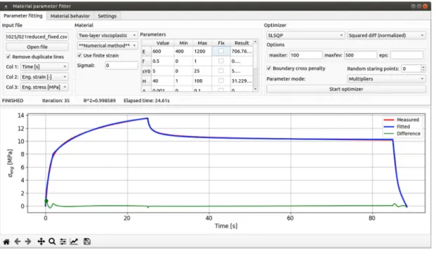
One of the primary goals in the parameter fitting procedure was to create a graphical interface, which can be easily used to calibrate the material parameters efficiently. We chose Python as our programming language as its open-source, cross-platform, and enables easier software development than some other tools. We utilized some of the commonly used modules (e.g. NumPy and SciPy) as well. The graphical user interface (GUI) was developed using the PyQt5 package. A screenshot about the program’s current version is shown in Fig. 5 where a particular fitting process is also visible.

5.2. Parameter-fitting problem

During the parameter-fitting process, the experimental values of the time, strain, and stress are given. The number of data points available is denoted with N. It should be noted that the experimental true stress values can be calculated if we can measure precisely the contraction of the specimen, which is usually a complicated task needing additional equipment. It should be emphasized that the adopted associative flow rule results in volume-preserving plastic deformation. In addition, for Fig. 2. Prescribed engineering strain history.

Table 1

Material parameters used for the comparison.

E [MPa] f [−] σ_Y0_[MPa] _{H [MPa]} _{A [MPa}⁻ⁿ_s⁻^m⁻¹_] _{n [}− ] m [− ]

1000 0.5 50 20 10⁻⁷ 3 − 0.5

Fig. 3.Calculated true stress values versus time.

Fig. 4. Calculated true stress values versus true strain.

(6)

polymer materials, the Poisson’s ratio of the material is close to 0.5 therefore, the overall volume-preserving deformation is a good approximation. Thus, assuming constant volume, one can determine the true stress from the engineering stress as

σ= (1+e)P. (30)

For steels, the Poisson’s ratio is about 0.3, but as the plastic deformation evolves, the overall Poisson’s ratio converges to 0.5.

There are different recommendations for measuring the quality of the fitting, or more precisely, the difference between the experimental data and the model prediction. One widely used quality function is the square root of the mean of the squares of the deviations:

Q=

̅̅̅̅̅̅̅̅̅̅̅̅̅̅̅̅̅̅̅̅̅̅̅̅̅̅̅̅̅̅̅̅̅̅̅̅̅̅̅̅̅

1 N

∑^N

i=1

(P^exp_i − P^sim_i )₂

√√

√√ , (31)

where P^exp_i is the experimental value for the engineering stress at the ith data point, whereas P^sim_i denotes the simulated model response at the same data point (see Fig. 6). In our analysis we employ this quality function for the optimization.

The current material model has 7 parameters, which needed to be calibrated during the optimization routine. This value might be considered as a large number of material parameters, leading to un- certainty and ambiguous solutions during the parameter-fitting process.

However, it should be emphasized the different material parameters represent different physical phenomena. In general, one cannot represent the same material characteristics with a different set of material parameters in this case. The primary goal within the optimization task is to find the global minimum for Q. It is evident there is no guarantee we can find this minimum. However, the properly chosen initial values and bounds for the parameters can significantly foster finding the global minimum.

In addition, it is possible to fit the pure elastic-plastic material response to the experimental data using a loading history with a very low strain-rate. In this case, the viscoelastic contribution can be

eliminated from the constitutive response. After fitting the elastic-plastic response, one can focus on the viscoelastic parameters’ calibration using new experimental tests with different applied strain-rates. Abaqus also recommends this strategy.

The proposed method can be easily adapted for the case when multiple experimental tests are available. It is a straightforward task to construct a quality function, which includes the errors resulting from each experiment. One can improve the accuracy of the fitting by including more than one experimental test in the construction of the quality function.

5.3. Functionality and code structure

The user can load measurement data and set up the optimization on the interface. Among others, the setup includes the initial guess for the parameters, fixing the value of some parameters, and changing the optimization algorithm or quality function. Additionally, the user can calculate the material behavior for fixed parameters and for specified time-strain history. This is a useful feature for making performance comparisons or analyzing the effect of each parameter. The horizontal axis of the plot can be changed between displaying time or engineering Fig. 5.Graphical interface of the calibration software.

Fig. 6.Illustration of the error between the experimental data and the simulation result.

(7)

strain.

The effect of each setting and the usage of the software is not discussed in detail in this paper. The software will be free to download for researchers with a complete user guide and tutorial.

The source code is structured in a modular fashion, making new additions easier. New material models or new numerical methods for the existing models can be defined, and they will automatically appear and work on the interface. The modular structure also helps with main- tainability, as the code is split into smaller sections.

5.4. Parameter handling

As described earlier, our TLVP model contains 7 material parameters, which can differ significantly in orders of magnitude. This is quite detrimental for the optimization algorithms.

Two alternative parameter handling modes were implemented to mitigate this issue. These are discussed below.

Scaling Method: In this mode, each parameter is scaled by a unique factor. These factors are given via the initial guess values for the optimizer. By estimating the orders of magnitudes correctly, the values

“seen” by the optimizer remain much closer to each other. It is not required to specify parameter boundaries in this mode. Our tests indi- cated that this way of handling the parameters is superior to using the

“raw” values in almost every test case. Usually, using the scaling mode significantly reduced the number of iterations and function evaluations needed to find the optimum, and in case of some algorithms, it considerably decreased the chance of not finding the optimum.

Normalization Method: Our second approach was to use a linear transformation to convert the parameters into the interval [0, 1] based on their boundaries. The lower boundary is transformed to 0, the upper boundary to 1. Naturally, it is necessary to specify the parameter boundaries for this method to work properly. This method also performed much better in our tests than the “raw” values. It varied between test cases if the scaling or normalization method performed better. As their results were overall similar, it cannot be determined which approach is “better”.

5.5. Algorithms

Our software supports several optimization algorithms provided by SciPy. They will not be discussed in detail in this paper, but some ob- servations made during our tests are noted here.

The constraints for the parameters are the following based on their physical or mathematical meaning: E>0, 1>f>0,A>0, n>0,0>

m>− 1, Y0>0,H>0.Not all algorithms can accept constraints for the parameter values. This is detrimental for two reasons. Firstly, the user cannot focus the optimization on the expected parameter ranges.

Secondly, crossing the limits mentioned above leads to physically non- admissible behavior. The numerical solution at these values may take considerably longer – even 10–50 times longer – than normal. To

“guide” these algorithms into the bounded zone, we penalize the quality function’s value outside the allowed range based on how many parameters are out of bounds.

The Sequential Least Squares Programming (SLSQP) algorithm was our main tool, as generally it was the fastest – if it was set up correctly.

Using one of the described alternative parameter handling modes is quite important for this algorithm, as it often failed to converge using the “raw” values. The Limited-memory Broyden–- Fletcher–Goldfarb–Shanno algorithm with bound constraints (L-BFGS- B) was usually slower but was more reliable in some tests. Both methods accept boundaries for the parameters.

The Powell algorithm was slower than the previously mentioned methods, but it performed well if the order of magnitude of the parameters was unknown. Unfortunately, it cannot handle parameter boundaries. The Nelder-Mead algorithm usually yielded good solutions, but it was considerably slower than the other algorithms. The Conjugate

Gradient (CG) algorithm was not the best in any test, but it might be viable in other cases, thus it is included in the program.

It is important to note, that this brief section does not aim to generally compare or rate these algorithms. It only records some ob- servations made during our tests.

6. Demonstration of applicability

To show the usefulness of the developed software, we have chosen some uniaxial measurement datasets from the literature.

6.1. Example 1 – MC-PET

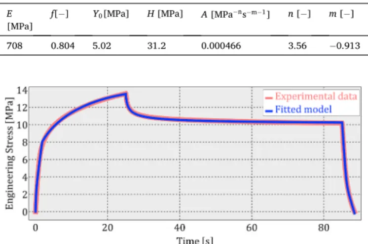
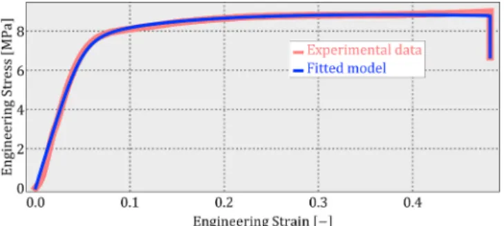
This dataset was chosen based on the author’s previous work and the availability of the original measurement data. In a series of experiments, microcellular polyethylene-terephthalate (MC-PET) polymer foam specimen were investigated at various temperatures [15]. We have chosen the uniaxial test at 21 ^◦C for this demonstration. The dataset consists of approximately 1500 points, all of them are used for the fitting. The fitted material parameters are listed in Table 2, whereas the comparison of the experimental data and the model response is depicted in Fig. 7 and Fig. 8. One can observe the excellent accuracy of the fitted Table 2

The calibrated material parameters for the MC-PET material.

E [MPa] f[−] Y0[MPa] H [MPa] A [MPa⁻ⁿs⁻^m⁻¹] n [−] m [− ]

708 0.804 5.02 31.2 0.000466 3.56 −0.913

Fig. 7.Comparison of the experimental data and the model prediction for the MC-PET material in Time Vs. Engineering Stress coordinate system.

Fig. 8.Comparison of the experimental data and the model prediction for the MC-PET material in Engineering Strain Vs. Engineering Stress coordinate system.

Table 3

The calibrated material parameters for the PFSA material.

E [MPa] f[−] Y0[MPa] H [MPa] A [MPa⁻ⁿs⁻^m⁻¹] n [−] m [− ]

160 0.926 0.619 85.9 3.87e-08 5.20 −0.523

(8)

model.

6.2. Example 2 – PFSA

In this measurement, perfluorosulfonic acid (PFSA) membranes were tested at various temperature and humidity levels [14]. The effect of the strain rate was also investigated. We have chosen the data measured at 26 ^◦C, 50% relative humidity and 2.6×10⁻⁵1/s initial strain rate. The dataset consists of approximately 160 data points. The material parameters we calibrated are listed in Table 3, whereas the comparison of the experimental data and the model response is depicted in Fig. 9 and Fig. 10. The fitted model gives excellent agreement with the experimental data.

6.3. Example 3 – P91 steel

In this measurement, the mechanical behavior of P91 steel specimen is investigated at elevated temperatures and different strain fluctuation amplitudes [23]. One of the reasons for including this dataset in our work is to test the software for a different type of material (metal, instead of polymer). We used the measurement performed at 400 ^◦C and 1% strain fluctuation (first cycle). The dataset consists of about 330 measurement points. The material parameters we have found using our software are given in Table 4. Fig. 11 and Fig. 12 show the comparison between the experimental data and the model predictions.

Based on the comparison above, one can conclude the measured initial apparent modulus is slightly higher than the fitted value for the instantaneous elastic modulus. The initial slope is around 210 GPa, but the fitted value is 180 GPa. This discrepancy can be resolved if one fixes the elastic modulus at the beginning of the optimization task. However, in that case, the overall quality of the fitting will be lower as we have no option to modify the elastic modulus to find a more accurate fit. If the

accurate representation of the elastic part is more important than the accurate characterization of the plastic part, then this method is advised.

6.4. Performance

We measured the performance of our software based on the elapsed wallclock time during the optimization. Naturally, this depends on the used hardware, the bottleneck being the single-core CPU performance due to the structure of the program. In most cases, the optimization was completed within 1–5 min. Noticeable improvements were rarely made after this timeframe. Sometimes switching algorithms could improve the fitting accuracy, but these improvements were usually minor. The parameter handling mode was set to “Scaling” during these tests. The initial guess can have a major impact on the performance of the algorithms. Appendix D contains a brief analysis of the performance of different optimization methods we investigated.

7. Conclusions

We have proposed an implicit time integration scheme for the two- layer viscoplastic model in one-dimensional uniaxial extension. The particular form of the material model consists of an elastic-plastic network governed by linear isotropic hardening rule, whereas the elastic-viscous branch in the model is equipped with a nonlinear time- hardening creep law. The one-dimensional representation of the Fig. 9. Comparison of the experimental data and the model prediction for the

PFSA material in Time Vs. Engineering Stress coordinate system.

Fig. 10. Comparison of the experimental data and the model prediction for the PFSA material in Engineering Strain Vs. Engineering Stress coordinate system.

Table 4

The calibrated material parameters for the P91 steel material.

E [GPa] f[−] Y0[MPa] H [GPa] A [MPa⁻ⁿs⁻^m⁻¹] n [− ] m [−]

180 0.712 189 7.28 7.7e-26 8.99 −0.0469

Fig. 11.Comparison of the experimental data and the model prediction for the P91 steel material in Time Vs. Engineering Stress coordinate system.

Fig. 12.Comparison of the experimental data and the model prediction for the P91 steel material in Engineering Strain Vs. Engineering Stress coordinate system.

(9)

model contains 7 material parameters, 4 among them corresponds to the elastic-viscous network. It was demonstrated that the proposed scheme produces the same result as the built-in material model in Abaqus.

However, our scheme is more stable, and we have not experienced any numerical difficulties during the time integration of a particular problem. The proposed algorithm was implemented in Python. A stand-alone calibration software was developed with a graphical user interface. The new program we constructed is freely available to download from the authors’ webpage. The performance of our calibration software was demonstrated by fitting the material parameters to three distinct experimental data sets from the literature. The fitted models revealed the excellent accuracy of the TLVP model in characterizing the mechanical behavior of the investigated materials. Due to the modular structure of the corresponding Python code, the software can be easily extended for more complex versions of the TLVP model (non-linear mixed hardening, for instance). The new calibration software may serve as a useful tool for researchers and engineers who want to fit the TLVP model to their experimental data.

It should be emphasized the demonstration examples we presented in the paper cannot be considered as a complete validation for the material model. For the validation task, it is crucial to fit the material model to different strain histories simultaneously, which can be easily achieved by modifying the quality function. One has to be sure the fitted parameters serve accurate material responses in other loading modes too.

Appendix E demonstrates a validation procedure for the MC-PET material. The performance of the fitted TLVP model is presented for a complex non-homogeneous loading case involving non-homogeneous strain-rate history in the material.

Contribution

Attila Kossa: Conceptualization, Methodology, Visualization, Inves- tigation, Writing – original draft, Writing – review & editing, Software, Andr´as Levente Horv´ath: Conceptualization, Methodology, Visualiza- tion, Investigation, Writing – original draft, Writing – review & editing, Software.

Declaration of competing interest

The authors declare that they have no known competing financial interests or personal relationships that could have appeared to influence the work reported in this paper.

Acknowledgments

This research was supported by the J´anos Bolyai Research Scholar- ship of the Hungarian Academy of Sciences; Hungarian National Research, Development and Innovation Office (NKFI FK 128662); the ÚNKP-20-5 New National Excellence Program of the Ministry for Inno- vation and Technology from the source of the National Research, Development and Innovation Fund. The research reported in this paper and carried out at BME has been supported by the NRDI Fund (TKP2020 IES, Grant No. BME-IE-NAT and TKP2020 NC, Grant No. BME-NC) based on the charter of bolster issued by the NRDI Office under the auspices of the Ministry for Innovation and Technology. The MC-PET foam specimens were provided by Furukawa Electric Institute of Technology (FETI) Ltd., Hungary, which support is gratefully acknowledged.

Appendix A. Wolfram Mathematica Notebook

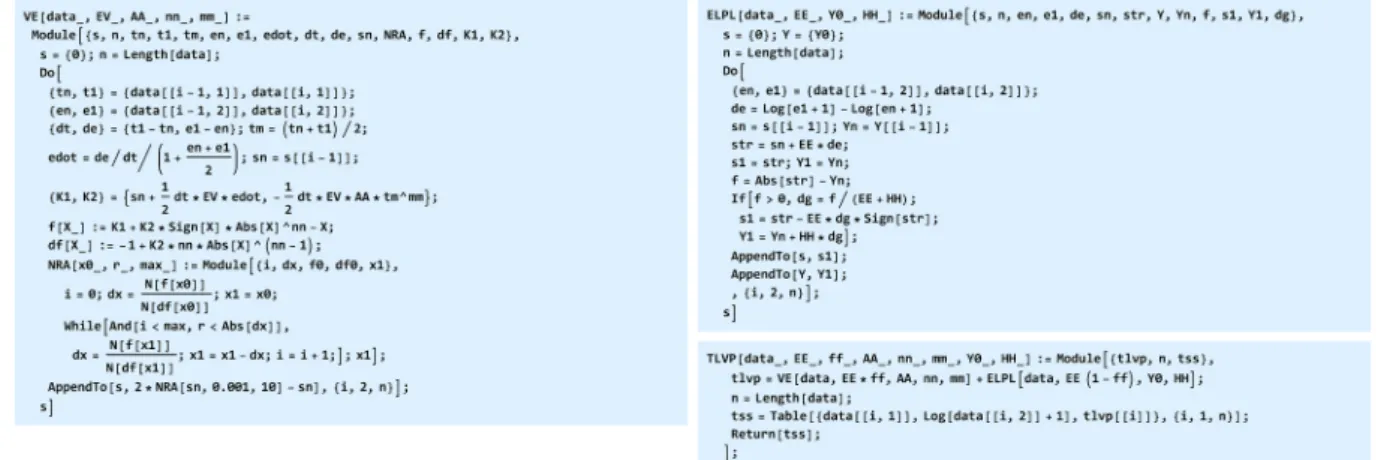
The Wolfram Mathematica module TLVP calculates the stress response for the uniaxial loading of a material characterized by the two-layer viscoplastic model. The input parameters are the prescribed engineering strain history and the material constants. The module calls two additional sub-modules, namely VE and ELPL, calculating the stress values in each network. Descriptions of the arguments in module TLVP are the followings:

Data: Tabular input for the strain history. The first column is the time value, whereas the second column is the engineering strain value.

EE, ff, AA, nn, mm, Y0, HH: These are the material parameters associated with the model, namely: E,f,A,n,m,Y0,H.

The code (see Fig. 13) uses fixed time increments defined by the input data. The output of the TLVP module is tabular data with the following columns: time, true strain, true stress.

Fig. 13.Wolfram Mathematica code for the two-layer viscoplastic model.

Appendix B. Abaqus input file

The plain Abaqus input file (Fig. 14) used for the uniaxial loading example in the validation section is given here. The finite element model consists of only one 8-node 3D linear brick element, as illustrated in Fig. 15. The coordinates and the prescribed displacement boundary conditions of the nodes are listed in the corresponding table. The displacement function u(t)in [mm] unit is equivalent to the history given in Fig. 2. A reduced integration scheme with one Gauss integration point is used because the resulting displacement field is homogeneous in the element.

(10)

Fig. 14.Abaqus input file for the validation example.

Fig. 15.Illustration of the FE model.

Appendix C. Analysis on parameter “cetol”

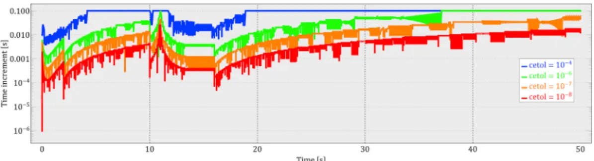
The following eight values were tested: 10⁻^k,wherek=1,2,3,4,5,6,7,8. The largest value for which the simulation was not terminated due to the convergence problem was 10⁻⁴. However, it is interesting to remark the calculations were terminated if we used the smaller value 10⁻⁵. For even smaller values, the simulations had no convergence issues. The software had to reduce the original time increment of 0.1 s significantly in order to be able to solve the problem. Fig. 16 shows the variation of the applied time increment size along the time for the four cases when the simulations were not terminated. It can be seen Abaqus was able to solve the problem with the maximum time increment of 0.1 s in a large domain when cetol =10⁻⁴ was used. However, for smaller tolerance values, the time increment was reduced significantly.

Fig. 16.Applied time increment size for different values of the viscoelastic strain error tolerance.

The average increment size, the total number of increments and the corresponding computation times are reported in Table 5

(11)

Table 5

Effect of the cetol value on the increment size and on the computation time.

cetol value Mean value of the time increments [s] Total number of increments Computation time [s]

10⁻⁴ 0.05086 983 31

10⁻⁶ 0.01091 4584 124

10⁻⁷ 0.003578 13973 355

10⁻⁸ 0.001160 43096 1375

Appendix D. Performance

The performance of the algorithms was compared for each example we investigated. For illustration purposes, the result for Example 1 is shown in Fig. 17, where empty circles indicate the end of a particular fitting procedure. Algorithms BFGS, L-BFGS-B and CG converged to the same parameter set with the same quality function, whereas the Nelder-Mead algorithm terminated at a quality function slightly above the previous value. The remaining two methods found local minima with a higher value of the quality function.

Fig. 17.Number of function evaluations over time. Variation of the quality function for different algorithms.

It is hard to determine general trends based on results. The efficiency of each algorithm can depend on the problem and on the initial guess values, for instance. However, it can be clearly concluded that different algorithms may serve different fitted values and, therefore, a different quality function value.

It is interesting to note that a significant proportion of the total time needed for the optimization process is not spent on evaluating the material behavior. Instead, it is consumed by the internal calculations of the optimizer algorithms itself. The shorter the material evaluation time, the more pronounced this effect gets. An illustration can be seen in Fig. 18. for Example 1. Note that the function evaluation rate does not correlate with the final quality of the fitting.

Fig. 18. Number of function evaluations over time MCPET.

We can also investigate the behavior of the algorithms with regard to the variation of the parameters during the minimization procedure. This is illustrated in Fig. 19 for Example 2 using the Nelder-Mead method. The parameter values are normalized on the plot, so their maximum value is 1 and minimum values is 0.

Fig. 19.Variation of the normalized material parameters during the calibration for Example 2 using the Nelder-Mead algorithm.

(12)

Appendix E. Validation of the fitted model for the MC-PET material

The TLVP model fitted for the MC-PET material shows excellent accuracy in the uniaxial test used for the calibration process. However, there is no guarantee the fitted model provides accurate characterization of the material in other loading cases. In order to validate the fitted model, we performed a complex loading experiment and compared the simulation result to the experimental data. A circular specimen was fixed along its perimeter, and a spherical steel head was used to deform the material with a prescribed vertical loading history u(t)containing loading, relaxation and unloading segments (see Fig. 20). This setup ensures a non-homogeneous deformation in the material with a non-homogeneous strain-rate distribution. Besides, it is important to emphasize the stress state is more likely biaxial rather than uniaxial. Consequently, the conditions for this test is very different than the uniaxial experiment used for the model calibration.

Fig. 20.Experimental setup for the punch test.

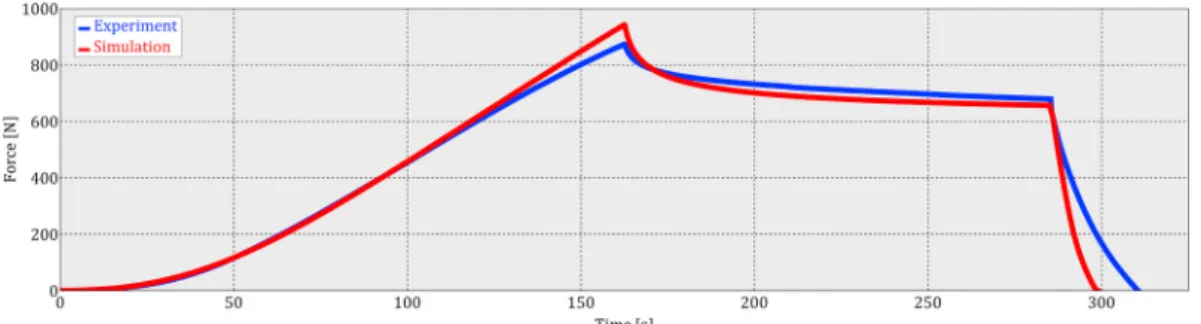
The FE simulation was performed using 8-node biquadratic axisymmetric quadrilateral elements with full integration scheme. Mesh dependency analysis was carried out to find a proper mesh density for the calculation. The final element size was 0.094 mm. The steel head was modelled using an analytical rigid surface as the head’s stiffness is significantly higher than the stiffness of the specimen. The friction coefficient between the head and the material was set to 0.15 but it should be noted it has negligible effect on the reaction force as the main contribution in the loading force is the force needed to deform the specimen. The material parameters for the TLVP model are listed in Table 2. The reaction force acting on the head is chosen for the comparison as it encapsulates the specimen’s overall mechanical behavior. Fig. 21 shows the experimental and the simulation results. One can conclude the material model used for the simulation can accurately represent the investigated material’s characteristics in this complex loading case.

This comparison demonstrates the applicability of the fitted model in other loading cases. The accuracy can be improved by fitting the material model to multiple experiments simultaneously as discussed in the conlucison section.

Fig. 21.Comparison of the experimental and simulation results for the force history.

The “cross-section” of the specimen’s deformed configuration after complete unloading is depicted in Fig. 22. The deformed shape has excellent agreement with the experimental observation as illustrated in Ref. [17] in a similar test using slightly different geometries.

Fig. 22.Deformed configuration after unloading. The straight segments correspond to the fixed region.

References

[1] Dassault Systemes Abaqus Version 2019, 2020.

[2] J. Kichenin, Comportement Thermomécanique du Polyéthylène—Application aux Structures Gazières, Mécanique et Matériaux, Spécialité, 1992. Thèse de Doctorat de l’Ecole Polytechnique.

[3] J. Kichenin, K. Van Dang, K. Boytard, Finite-element simulation of a new two- dissipative mechanisms model for bulk medium-density polyethylene, J. Mater.

Sci. 31 (1996) 1653–1661, https://doi.org/10.1007/BF00357878.

[4] J. Kang, A. Becker, W. Sun, Determination of elastic and viscoplastic material properties obtained from indentation tests using a combined finite element analysis and optimization approach, Proc. Inst. Mech. Eng. Part L J. Mater. Des. Appl. 229 (2015) 175–188, https://doi.org/10.1177/1464420713504534.

[5] L. Figiel, B. Günther, Modelling the high-temperature longitudinal fatigue behaviour of metal matrix composites (SiC/Ti-6242): non-linear time-dependent matrix behaviour, Int. J. Fatig. 30 (2008) 268–276, https://doi.org/10.1016/j.

ijfatigue.2007.01.056.

(13)

[6] E. Charkaluk, A. Bignonnet, A. Constantinescu, K. Dang Van, Fatigue design of structures under thermomechanical loadings, Fatig. Fract. Eng. Mater. Struct. 26 (2003), https://doi.org/10.1046/j.1460-2695.2002.00613.x-i1, 661–661.

[7] S.B. Leen, A. Deshpande, T.H. Hyde, Experimental and numerical characterization of the cyclic thermomechanical behavior of a high temperature forming tool alloy, J. Manuf. Sci. Eng. 132 (2010) 304–313, https://doi.org/10.1115/1.4002534.

[8] M. Saber, W. Sun, T.H. Hyde, Numerical study of the effects of crack location on creep crack growth in weldment, Eng. Fract. Mech. 154 (2016) 72–82, https://doi.

org/10.1016/j.engfracmech.2016.01.010.

[9] T.P. Farragher, S. Scully, N.P. O’Dowd, S.B. Leen, Thermomechanical analysis of a pressurized pipe under plant conditions, J. Pressure Vessel Technol. 135 (2013) 1–9, https://doi.org/10.1115/1.4007287.

[10] T.P. Farragher, S. Scully, N.P. O’Dowd, C.J. Hyde, S.B. Leen, High temperature, low cycle fatigue characterization of P91 weld and heat affected zone material, J. Pressure Vessel Technol. 136 (2014) 1–10, https://doi.org/10.1115/1.4025943.

[11] T. An, R. Selvaraj, S. Hong, N. Kim, Creep behavior of ABS polymer in temperature–humidity conditions, J. Mater. Eng. Perform. 26 (2017) 2754–2762, https://doi.org/10.1007/s11665-017-2680-0.

[12] J. Doh, S.H. Hur, J. Lee, Viscoplastic parameter identification of temperature- dependent mechanical behavior of modified polyphenylene oxide polymers, Polym. Eng. Sci. 59 (2019), https://doi.org/10.1002/pen.24910. E200–E211.

[13] A.A. Abdel-Wahab, S. Ataya, V.V. Silberschmidt, Temperature-dependent mechanical behaviour of PMMA: experimental analysis and modelling, Polym.

Test. 58 (2017) 86–95, https://doi.org/10.1016/j.polymertesting.2016.12.016.

[14] R. Solasi, Y. Zou, X. Huang, K. Reifsnider, A time and hydration dependent viscoplastic model for polyelectrolyte membranes in fuel cells, Mech. Time- Dependent Mater. 12 (2008) 15–30, https://doi.org/10.1007/s11043-007-9040-7.

[15] S. Berezvai, A. Kossa, Performance of a parallel viscoelastic-viscoplastic model for a microcellular thermoplastic foam on wide temperature range, Polym. Test. 84 (2020) 106395, https://doi.org/10.1016/j.polymertesting.2020.106395.

[16] S. Berezvai, A. Kossa, Characterization of a thermoplastic foam material with the two-layer viscoplastic model, Mater. Today Proc. 4 (2017) 5749–5754, https://doi.

org/10.1016/j.matpr.2017.06.040.

[17] S. Berezvai, A. Kossa, A.K. Kiss, Validation method for thickness variation of thermoplastic microcellular foams using punch tests, 36th Danubia Adria Symp, Adv. Exp. Mech. DAS 32 (2019) (2019) 83–84, https://doi.org/10.1016/j.

matpr.2020.02.977.

[18] A.G. Reisinger, M. Frank, P.J. Thurner, D.H. Pahr, A two-layer elasto-visco-plastic rheological model for the material parameter identification of bone tissue, Biomech. Model. Mechanobiol. 19 (2020) 2149–2162, https://doi.org/10.1007/

s10237-020-01329-0.

[19] Dassault Systemes Isight Version 2019, 2020.

[20] R.I. Borja, Plasticity, Springer, 2013, https://doi.org/10.1007/978-3-642-38547-6.

[21] E.A. De Souza Neto, D. Peri´c, D.R.J. Owen, Computational methods for plasticity:

theory and applications. https://doi.org/10.1002/9780470694626, 2008.

[22] A. Kossa, L. Szab´o, Exact integration of the von Mises elastoplasticity model with combined linear isotropic-kinematic hardening, Int. J. Plast. 25 (2009) 1083–1106, https://doi.org/10.1016/j.ijplas.2008.08.003.

[23] T.P. Farragher, S. Scully, N.P. O’Dowd, C.J. Hyde, S.B. Leen, High temperature, low cycle fatigue characterization of P91 weld and heat affected zone material, J. Pressure Vessel Technol. 136 (2014) 1–10, https://doi.org/10.1115/1.4025943.