Evaluation of climate change scenarios based on aquatic food web modelling

(1)

EVALUATION OF CLIMATE CHANGE SCENARIOS BASED ON AQUATIC FOOD WEB MODELLING

CS.VADADI-FÜLÖP¹*–L.HUFNAGEL²–CS.SIPKAY²–CS.VERASZTÓ¹ 1Department of Systematic Zoology and Ecology, Eötvös Loránd University,

H-1117 Budapest, Pázmány P. sétány 1/c, Hungary

2Department of Mathematics and Informatics, Corvinus University of Budapest, H-1118 Budapest, Villányi út 29-33, Hungary

(phone: +36-1-372-6261; fax: +36-1-466-9273)

*e-mail: vadfulcsab@gmail.com

(Received 30^th September 2007; accepted 15^th November 2007)

Abstract. In the years 2004 and 2005 we collected samples of phytoplankton, zooplankton and macroinvertebrates in an artificial small pond in Budapest. We set up a simulation model predicting the abundance of the cyclopoids, Eudiaptomus zachariasi and Ischnura pumilio by considering only temperature as it affects the abundance of population of the previous day. Phytoplankton abundance was simulated by considering not only temperature, but the abundance of the three mentioned groups. This discrete-deterministic model could generate similar patterns like the observed one and testing it on historical data was successful. However, because the model was overpredicting the abundances of Ischnura pumilio and Cyclopoida at the end of the year, these results were not considered. Running the model with the data series of climate change scenarios, we had an opportunity to predict the individual numbers for the period around 2050. If the model is run with the data series of the two scenarios UKHI and UKLO, which predict drastic global warming, then we can observe a decrease in abundance and shift in the date of the maximum abundance occurring (excluding Ischnura pumilio, where the maximum abundance increases and it occurs later), whereas under unchanged climatic conditions (BASE scenario) the change in abundance is negligible. According to the scenarios GFDL 2535, GFDL 5564 and UKTR, a transition could be noticed.

Keywords: hydrobiology, community, ecosystem, climate change

Introduction and aims

The concept of seasonal dynamics is published in several forms. It has been come out like „seasonal variation”, seasonal changes” or „seasonal cycle” considering changes in the abundance, biomass or in the composition of assemblage. From our point of view, seasonal dynamics is temporal change in the examined assemblage, which is regulated by the climate, primarly by the temperature. It has been shown that abundance and structure of the zooplankton community display considerable variations on seasonal, interannual, and regional scales (Arashkevich et al., 2002). Predictable patterns of biodiversity often occur in freshwater pelagic communities over yearly cycles in temperate regions of the globe (Bernot et al., 2004).

Zooplankton is a crucial component of aquatic ecosystems because of its role in the trophic chain. It represents the channel of transmission of the energy flux from the primary producers to the top consumers (Abrantes and Goncalves, 2003). Many species of zooplankton serve as feed for fishes, moreover they could be keystone species.

Copepoda is one of the most important groups of freshwater zooplankton and is one of the most numerous animal groups on the earth, occurring in all types of freshwater bodies. The phytoplankton as primary producers make it possible to operate the aquatic ecosystem in that way, they accept the solar energy and serve as feed.

(2)

Our main aims were the following:

• Description of the phytoplankton, zooplankton and macroinvertebrate assemblages in the examined pond.

• Working out and adopting a sampling method regularly carried out, that provides accurate data of the temporal change of the examined objects.

• Elaborate a simple simulation model, which is able to generate similar patterns to the observed ones. Testing the model.

• Running the model with the data series of different internationally recognized climate change scenarios, supplying and interpreting of the predictions.

Comparative estimating of the alternative climate change scenarios with classical statistical methods.

We chose an artificial and small pond to examine, as we thought it is simpler and more closed than natural freshwaters, and the operation of the system could be easier understood. We expected the model to indicate real patterns like the observed data series, thus the climate change scenarios could be valued. By means of a simple simulation model we were able to generate similar patterns like the observed one.

Running the model with the data series of different climate change scenarios, we got a prospective notion of the abundance of the examined objects, which must be handled watchful. The aim of the process is not the prediction, but the comparative appreciation of the possible effects of the different, international climate change scenarios, with the aid of a real model situation.

Review of literature

Climate change, climate change scenarios

Climate change is considered, when the fluctuation range of climatic elements shifts appreciably to the higher or lower values, and this state remains for a long period (Varga-Haszonits, 2003). General Circulation Models (GCM) were developed at first to modelling the atmosphere’s processes. Later also the atmosphere’s interactions with biosphere, hydrosphere, litosphere and criosphere were taken into consideration, and these models were accounted as Global Climate Models (GCM). These models use 3D space, tracking horizontal and vertical movements and cover the surface with grid (Varga-Haszonits, 2003). Two types of GCM are distinguished: equilibrium and transient models. The equilibrium model calculates with doubled level of carbon-dioxid in the atmosphere. The model is run till then it set in an equilibrium state, namely a state when it evolves a stable temperature on the surface. By gradually increasing level of carbon-dioxid, transient models make it possible to determine the gradually changing climatic conditions (Varga-Haszonits, 2003). The claim to apply GCM for regional levels demands using the method of downscaling. The kernel of downscaling is considering the results of GCM’s for great areas, and setting statistical correspondence between the climatic variables of great and minor areas (Varga-Haszonits, 2003).

Climate change scenario can be defined as a likely combination of the change of climatic conditions, which is able to use for testing the possible effects and asses the reactions for them (Varga-haszonits, 2003). These models are based on the simulations of General Circulation Models and regional climate models. Some remarkable institutes for developing GCMs are the undermentioned: the Geophysical Fluid Dynamics Laboratory (GFDL), the Goddard Institute for Space Studies (GISS), the National

(3)

Center for Atmospheric Research (NCAR) and the United Kingdom Meteorological Office (UKMO). Scenarios are doubtful, so it is rewarding and also common to use alternative scenarios in the studies. Scenarios do not give factual forecasts, rather make hypothetical prospects. Leastwise they are useful for biophysical and socioeconomic systems, by giving the trend and amplitude of changes and giving the threshold of processes that are sensible for climate (Varga-Haszonits, 2003).

The scientific results concerning climate change are summarized in IPCC (Intergovernmental Panel of Climate Change) reports. Hungary takes part in this program too. For the sake of global warming and climate change VAHAVA project was started in Hungary. Its primary aims were to get ready for the negative or positive effects of global climate change, prevention of loss, mitigation of damage and forwarding of restoration (Láng et al., 2006).

Seasonal dynamics of zooplankton

In Hungary Lake Balaton is one of the most investigated freshwaters. The Balaton Limnological Research Institute has been monitoring the qualitative and quantitative change of zooplankton in Lake Balaton for a long time. Based on its data series, the abundance of Crustacean plankton increased until 1951, then decreased gradually until 1965 (it was the year when a lot of fish perished), just in the late sixties was observed moderate rising in abundance. Eudiaptomus gracilis came out at 25-50% of total Crustacean plankton in Lake Balaton in 1996-1997 (Zánkai and Ponyi, 1997). The quantitative changes of Eudiaptomus gracilis were described by Ponyi, Horváth and Zánkai (1975). There is a great difference, both quantitatively and qualitatively, between the samples collected in July and in September: the abundance of copepods increases in September, whereas the abundance of cladocerans decreases (Ponyi and Tamás, 1964). Ponyi et al. (1974) examined a fishpond near by Lake Balaton and they found maximum biomass in early summer and it decreased in July. Only in June was the biomass of Cladocera significant, in July it was less and then this group disappeared.

In early summer copepod biomass was less than cladocerans biomass, but copepods remain with high abundance after disappearing of Cladocera.

Seasonal and daily patterns of zooplankton populations are often predictable in natural lakes (Bernot et al., 2004). According to Wu and Culver (1994), food and predation were the two main factors regulating Daphnia population dynamics. Mouny and Dauvin (2002) studied the dynamics of mesozooplankton in the Seine estuary. The marine species showed maximum abundance at the end of spring, while freshwater species peaked in summer correlated with the maximum water temperature. One copepod species dominated the zooplankton throughout the year. In Sommer’s opinion (1989) seasonal succession of planctonic communities is driven by the changing availability of limiting resources to phytoplankton and zooplankton populations. In zooplankton seasonal succession, communities of a few large species give way to communities of smaller, more diverse s in late spring or early summer (Sommer, 1989;

Caceres, 1998). Simona et al. (1999) did not find seasonal succession in a mountain lake in the Alps. From the article written by Ferrara, Vagaggini and Margaritora (2002) we are able to form a notion of zooplankton, dominated by an Eudiaptomus species, where cladocerans peaked in summer and in autumn.

Previous references were concerned freshwaters, however most publications which we have found, deal with seas. Landry et al. (2001) found statistically significant seasonal signals, with peak biomass and abundance during the summer months for the

(4)

mesozooplankton community at Station ALOHA on the Pacific Ocean. There may have been an increase of about a factor of two in zooplankton standing stocks over the past two decades and the authors presume, that nitrogen fixation could provide the source of new nutrients to support higher productivity, larger phytoplankton, and enhanced zooplankton standing stocks in the summer, when the upper water column is most stratified and isolated from nutrient influxes from below. Arashkevich et al. (2002) did not find considerable changes in zooplankton biomass between seasons in the Barents Sea. There is a seasonal succession in San Francisco Bay, involving the replacement of a cold-season species by a warm-season species, and the zooplankton abundance appear to be constant among years (Ambler et al., 1985). The seasonal dynamics was discussed in relation to temperature, coastal hydrography and the seasonal cycles of phytoplankton. Christou (1998) examined the abundance of copepods in a Mediterranean coastal area (Aegean Sea) during five years. Copepod abundances and environmental parameters, almost all, exhibited pronounced annual cycles, and most copepods revealed repeated patterns and considerable interannual variability.

Temperature and salinity were the most significant environmental parameters accounting for the variability of abundances. According to Ikauniece (2001) the abundance of coastal mesozooplankton species in the Gulf of Riga is determined by the combination of hydrological regime, predation pressure, benthic conditions and the success of living strategy. Kovalev et al. (2003) summarized the zooplankton seasonal dynamics of the Mediterranean, the Black and the Azov seas, based on their own data and data from literature. In the deep water central regions of the seas, the seasonal cycle of zooplankton abundance is characterized by one maximum occurring in spring or summer. In the coastal regions, two or three peaks (spring, summer and autumn) exist.

The amplitude of seasonal fluctuations increases from the Mediterranean to the Black and Azov seas, as well as from South to North in each sea. The results of Dippner, Kornilovs and Sidrevics (2000) suggest that in the Central Baltic Sea the interannual variability during spring of zooplankton species is controlled by the sea surface temperature during spring (significant correlation was found only in spring). A possible explanation for it is the top-down control by fishes (smaller feeding activity in spring).

Chiba and Saino (2003) examined the effect of El Niño events on the zooplankton community in the Japan Sea. They observed a clear seasonal succession in community structure from a cold-water copepod-dominated community in winter and spring to a gelatinous, carnivorous and warm-water copepod-dominated community in summer and autumn. The spring community structure varied considerably between years. Iguchi (2004) collected the knowledge of Japan Sea concerning zooplankton in his review he also presented results about seasonal dynamics. Temporal variations in zoopankton biomass showed both seasonal and year-to-year components, maximum abundances occured in spring. As for long-term changes, 3-6 year cycles were identified, with the dynamics of the surface warm Tsushima Current and the subsurface cold water.

Dolganova and Zuenko (2004) found no significant inter-decadal variation, but interannual variation was considerable and generally opposite to water temperature changes in the upper layer of the Japan Sea. The pattern of zooplankton productivity is changing over time in the subarctic Pacific, probably in response to interdecadal ocean climate variability (Mackas and Tsuda, 1999). These changes include 2-3 fold shifts in total biomass, 30-60 day shifts in seasonal timing, and 10-25% changes in average body length.

(5)

Publications concerning specifically modelling were not available in force. Generally complex approaches are typical: considering predators, food, environmental parameters jointly. We did not find any articles dealing with the modelling with climate change scenarios in the literature of zooplankton. Angelini and Petrere (2000) set a modell to describe the plankton system of the Broa reservoir. The three state variables of the model were: phytoplankton, zooplankton and the fish Astyanax fasciatus. The forcing variables were: temperature, nitrate, phosphorus and solar radiation. According to their results, temperature was the most important variable in the system. Broekhuizen et al.

(1995) dealt with the modelling the dynamics of the North Sea’s mesozooplankton.

Among the parameters there were nutrients, detritus, carnivorous and omnivorous mesozooplankton, microzooplankton, flagellates and diatoms.

Seasonal dynamics of macroinvertebrates

There are many references in the literature that the quality and quantity of submerged and emerged macrophytes may play an important role in the spatial and quantitative patterns and the combination of species of the macroinvertebrate fauna (Müller et al., 2001), thus the relevance of examining macrophyte is indisputable.

Müller et al. researched parts of Lake Tisza with narrowleaf cattail and other aquatic plants (Müller et al., 2001). According to their results areas with narrowleaf cattail stands contained the most species and this area also proved to be the richest from the aspect of spiders, insects and mayflies.

Nicolet et al. researched wetland plants, macroinvertebrate s and the water’s physico- chemical characteristics of 71 temporary ponds in England and Wales (Nicolet et al., 2004). Their work primarily directs attention to the importance of temporary ponds from the point of view of nature conservation.

Parson and Matthews’ work (1995) emphasizes the relation between the macroinvertebrates and the macrophytes, pointing out that this is an insufficiently researched subject in water systems. The authors examined the invertebrate macrofauna of emergent macrophytes and submerged macrophytes in a small, shallow, eutrophic pond in the USA.

The scientific knowledge accumulated over the years made Lake Balaton one of the most thoroughly researched shallow lakes in the world. However earlier works are characterized by the fact that they neglected seasonal dynamics (Sipkay, Hufnagel and Gaál, 2005). In recent years Muskó et al. (2004) took quantitative samples of macroinvertebrates for three years in the submerged macrophyte stands of the north shore of Lake Balaton using the sampling method and device described by Bíró and Gulyás. During this research seasonal dynamics were also studied. During a year they took samples on a total of three (May-June, July and October) occasions and in another year they took samples on four occasions (May, July, September and October). Because of the methodology they used, their results are comparable with data gathered in much earlier years.

In the scientific literature there are references to the seasonal changes of certain groups that make up the invertebrate macrofauna of Lake Balaton. Seasonal dynamics of certain groups of Balaton invertebrates on offshore bars have also been investigated by Dózsa-Farkas et al. (1999). Data about the seasonal fluctuation of certain invertebrates living in settlings and being a part of the fish nutrition were provided by Szító (1998).

(6)

In their previous work, Sipkay and Hufnagel (2006) attempted to model the seasonal changes of Limnomysis benedeni. The model generated simulated data based on the daily mean temperature and the water level as imputs. They used the same method for optimizing the parameters. Our model is based on this work partly.

Phytoplankton succession

The research of phytoplankton has begun in the 19^th century, accordingly a lot of calculable information has been gathered during this period, though exploring a lake requires years of work. Using the reverse microscope developed by Utermöhl (1958) surveys of phytoplankton has been boomed. The first time series’ were described in the 40-s and 50-s, but detailed surveys concerning zooplankton and water chemical variables, were just reported in the 60-s (for instance Nauwerck 1963). During this period the phytoplankton succession has become a pregnant phenomenon among hydrobiological surveys. Therefore many remarkable works have been conducted by now, but interpreting and associating these works is complicated. It is not surprising, that the first model dealing with the plankton succession (the so-called PEG-model [Plancton Ecological Group]) was sketched just to 1986, as a result of the synthesis of many case studies (Sommer et al., 1986). The applicability of this model revealed, that many types of lakes should be distinguished in the aspect of plankton, as the PEG- model is adapted only for modelling the plankton succession of the temperate, deep lakes. It is crucial to note, that in Hungary there is no natural stratified deep lake, therefore there is no general model for it.

In shallow lakes it can not evolve temperal and water chemical stratification, even so it does not exceed the secondary water chemical stratification of epilimnion, occurring in natural deep lakes.

At first in the 60-s it was recognized, that hypertrophication is traceable by determining the biomass and production of phytoplankton. Vollenweider (Vollenweider 1968; Vollenweider & Kerekes, 1982) was the first who said that the reason for eutrophication is the increasing quantum of nutrients (principally phosphorus).

Researchers working in 70-s, like Somlyódi et al. (1983), handled phytoplankton as one variable, and tried to explore the background functions, though phytoplankton does not exist, it consists of many species evolved in different ways and are grouped in the way of community dynamics.

Such complex models set up in the 60-s, were followed simpler models (Jorgensen, 1994). The community approach were not detailed enough, parametrization was set back by differentiating only seven functional groups (Jörgensen & Padisák, 1996).

Tilman (1982; Tilman et al., 1982) showed a new way labouring his source- allocation models, where certain population dynamics changes were able to interpret.

Namely if we want to defend against algal bloom, we should know the main community dynamics except the autecological parameters of the given species.

According to the competitive exclusion principle, succession leads to the climax state with low diversity (Hardin 1960). Therefore it can be said, that in the temperate regions the equilibrium state is characterized by the dominance of 1-3 species, because phytoplankton is limited in this regions only by 1-3 source together (phosphorus, nitrogen, silicon, light). However, much more species occurs in the phytoplankton community together. This is the so-called paradox of plankton, formulated first by Hutchinson (1961). Hutchinson surmised that the solution is changing the boundary

(7)

conditions, but it was first described by Richerson et al. (1970) as „contemporaneus disequilibrium”.

Connel (1978) supposed that the competitive exclusing principle is not effective (if it exist). Communities with a lot of species never get to the climax state with low species richness, because of the disturbations. This presumption was formulated as the Intermediate Disturbance Hypothesis (IDH).

It should be mentioned the comparative works in the last decades, which tried to contrast models set up for phytoplankton with models set up for terrestric communities.

After many works an approach was stood out, that a minor break in the weather, which is negligible for the offsore vegetation, can be up to a climate change for phytoplankton (Sommer et al. 1993).

Elton (1927) has already pointed out that terrestrial and aquatic communities should function uniformly. In this wise there is a parallelism with models worked out for terrestrial systems. Nevertheless Cohen (1994) pointed the inverse trait of this comparison. As long as we examine phytoplankton among its own spatial and temporal traits, then the survival, growth, community organization and succcessional evolution of the species answer all the criteria (Padisák, 1985).

In Hungary Lake Balaton is the centre of limnological research. According to Padisák (1985) the nutrient proportion and secondary stratification (during the long calm periods) are followed by the structural changes of phytoplankton. During calm periods between storms, diversity increases initially, then decreases. This means that after stiring small phytoplankton (<10 µm) occur, and 4-5 days later larger phytoplankton (> 10 µm) are multiplying.

DIVDROP method (Rajczy & Padisák, 1983) was used to determine the dominant species during algal blooms and also other cases (for instance: 1976-78 Aphanizomenon flos-aquae, after 1980 Cylindrospermopsis raciborskii). However species becoming dominant can not be predicted (Kalff & Knoechel, 1978).

The phytoplankton succession in Lake Balaton, in summer is operating according to the IDH. The diversity has maximum by medium frequency of disturbance, whereas by high or low frequency diversity is low (Padisák, 1993).

Vörös and Kis (1985) applied the Reynolds-periodicity (Reynolds, 1980, 1982) in their case study in Lake Balaton; the definition of succession is practicable only for terrestrial vegetation according to the authors. To start-up they used Margalef’s concept for succession (Margalef, 1960), which is supported by several studies performed on seas (Guillard & Kilham, 1977). The phases of Margalef’s succession are the following:

• Abundance is high, mainly the species with weak buoyancy and small size are dominant, however the nutrient concentration is outside.

• Appearing species with medium and large size, total abundance is decreasing, the quantum of nutrient is decreasing.

• Spreading and dominating species with large size, moderate developing and good buoyancy. These species are often toxic (Margalef, 1960). The nutrient concentration is minimal.

Previous conception is reasonable, since the reproduction rate (Fogg, 1965), the P/B ratio (Gutelmacher, 1975; Desertova, 1976) and the specific respiratory rate (Laws 1975, Banse, 1976) decrease by increasing size. Furthermore feeding rate is influenced by the size of the cells (Parsons & Takahashi 1973), therefore it woud be evident, that species with smaller size become dominant by expendable nutrients. However the opposite occurs in nature, so the size of the cells is not primarily determined by feeding

(8)

rate. There is another conception which seems to be more appropriate, namely small cells have high respiratory rate and deplete their nutrient reserve sooner than larger cells by stray nutrient source. Respiration and compensation of damages are key factors in species selection by plankton s. In this way, the restriction of phytoplankton succession in size change is an obligate but necessary simplification.

Cluster analysis performed by Vörös and Kis (1985) supported the phases of Margalef’s succession (Margalef, 1960). By regions with medium quantum of biomass, the winter and spring periods correspond to the first phase of succession, the late spring period corresponds to the second and the summer period corresponds to the third phase of succession. The autumn period is in accordance with the turning of this process, which is braken off by the winter. Such reversion is an elementary process in the change of species composition by phytoplankton (Reynolds 1980). The effect of reversion intensified in the most eutrophic area of Lake Balaton (Keszthely Bay) and prevented evolving the total succession. This phenomenon has been observed also at seas (Guillard & Kilham, 1977).

Vörös and Kis (1985) attracted attention to the lack of a general theory and to the necessity of size dependency, in addition searching for a simpler object could be useful in surveys.

Materials and methods Sampling site

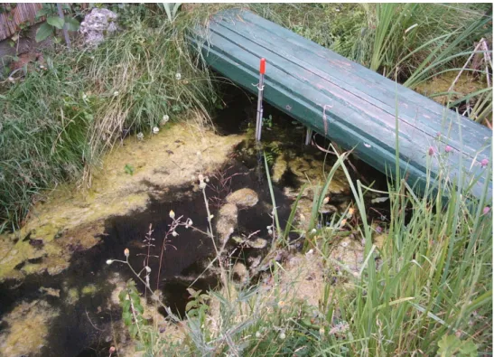
The sampling site was designated in an artificial small pond, located in Budapest, in a yard of a family residence (Fig. 1-2.). The climate is temperate and it is moderately shortage of rainfall. The mean yearly temperature is between 10.0-10.2 °C. The water surface is 522 dm², the depths is 30 cm. The bottom of the pond is covered by gravel and organic sediment. The water level was constant, there was no outflow. The evaporated water was replaced with water from the tap. During the whole survey no treatment was applied, no plants were removed. In winter the pond was frozen in, but it has never frozen in to the bottom.

The plants, animals and the sediment were introduced from a reach of Creek Szilas, opened up earlier with detailed examinations. Furthermore different creatures could colonize the pond from the air spreading passively, or actively from the soil or air. The northern part of the pond and its three corners were covered with plants (Fig. 3.). Trees were not present in the vicinity. The following plants were characteristics of the pond:

Iris pseudacorus, Carex acutiformis, Mentha aquatica, Myosotis palustris, Typha latifolia, Juncus effusus, Sium sp, Sparganium sp..

(9)

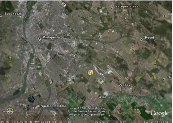
Figure 1.Distant record of the countryside. The sampling site is marked.

Figure 2. Near record of the countryside. The sampling site is marked.

(10)

Figure 3.Photograph of the examined pond taken in summer 2004.

Sampling method of zooplankton and processing of samples

The sampling was conducted weekly from March 2004 to October 2005, except in winter, when sampling was more infrequent because of the low abundance. In summer and in early autumn the abundance was high, therefore just the half or the quarter of the samples were processed, then data were multiplied by two or four. Zooplankton was sampled using a plankton net (17cm diameter, 250µm mesh size) always at the same mode. The sampling was representative, samples were taken systematicly from the whole water-column. 20 litres of water were filtered. Sample was immediately handled with heat water, this treatment prevents the planktonic organism from contraction, making it easier to identify them later. Afterwards sample was sorted in a laboratory under binocular microscope. Nauplii and Rotatoria were not determined. Identifying was performed to the closest taxa level. After sorting and counting, animals were preserved in formaldehyde, and some groups were identified later to species level.

Sampling method of macroinvertebrates and processing of samples

Sampling was performed biweekly from March 2004 to October 2005. Samples were taken from three locations.

• Underlay: collecting was conducted from three points of the pond (halfway and on the two ulterior brinks of the pond). The spit was a pot fixed to a handle.

During one bailing, the sediment and also water got into the pot. After sedimentation (it took few minutes) water was decanted partly, and the leftover was percolated. Percolation was carried out using a sieve with small mesh size, and also a strainer to avoid falling rough detritus into the sample. The filtrate was searched. The underlay was sampled three times at every turn.

(11)

• Water column: the spit was a strainer fixed to a long handle (1mm mesh size).

Samples were taken from different points of the pond by 6 bailings. Plants getting into the strainer were poured into a basin. After bailings, parts of the plants were leached with water-course (to the strainer). For other straining vide supra. In summer, because of the high abundance, sampling size was middled (3 bailings intead of 6).

• Surface of the water: animals observed on the surface, were counted and estimated.

Sampling method of phytoplankton and processing of samples

Pytoplankton was sampled by taking out x litre water of the pond from different points (the volume was not determined). With this 4X50cm³ water was taken out and spun with an ultracentrifuge. Then 4X5cm³ water get into a vessel and 3X1 drop from it is being examined.

Additional survey: taking out x litre water from different points of the pond and comparing the samples.

Simulation methods

For ecological modelling discretely represented time and deterministic simulation approach were applied in this work. Abundance was given daily (discrete), and the outcome leads to the same result at same conditions (deterministic). The predictions are valid only for the examined pond and at unchanged conditions (except temperature).

Zooplankton and Ischnura pumilio (macroinvertebrate) were simulated by considering only temperature and their abundance at the previous day, whereas phytoplankton were simulated by considering temperature and abundance of three other taxa (Ischnura pumilio, Cyclopoida, Eudiaptomus zachariasi). Calculations were made with MS Excel, and its Solver optimaliser programs.

Statistical analysis

Tukey-test was used to evaluate the results of the modelling. Scenarios and historical data series (see later) can be considered as treatments, therefore we can make a comparison between them with the mentioned method. Our question was, if there is any difference between the treatments (see Results). All statisical analysis was performed using Past software (version 1.36, Copyright Hammer and Harper 1999-2005).

Use of terms

• Climatic change scenario: a probable combination of the change of climatic conditions, which can be used for testing the possible effects and estimating the reaction on these changes (Varga-Haszonits 2003).

• Morphon: a category that takes into account the given animal’s taxonomical position, ontogenetical state and body size at the same time. The use of this category is justified for the investigation of seasonal dynamics, as here it is a clear concept.

• Seasonal dynamics: seasonal dynamics is temporal change in the examined assemblage (change in abundance, species composition, or biomass) which is regulated by the temperature among others.

(12)

• Simulation: creating artificial data series with mathematical models, which are reminiscent of data for temporal coenological state change.

• Simulation model: formulating hypothesis and conditions with mathematical methods concerning temporal state change.

• Zooplankton: in our work, zooplankton are animals kept by the plankton net used in our survey. This definition differs from that in the literature, but it is methodically more consistent.

Results

Faunistic overview

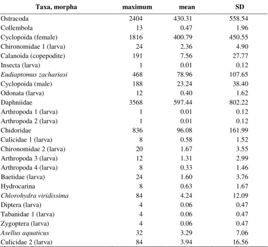
Table 1 shows the identified taxa and species occured in zooplankton samples. In the case of cyclopoids, we distinguished the males and females. Many animals were present as larvae. Contrary to the conventional definition of zooplankton, here are some taxa not belonging to zooplankton traditionally. Table 2 shows the identified taxa and species found in macroinvertebrate samples. Some groups are also present in zooplankton samples (such as Copepoda).

Table 1.The identified taxa (morpha) and species of the zooplankton samples, with the maximum abundance, mean and standard deviation values gathered during the survey. The values refer to the individual numbers found in 20 litre water.

Taxa, morpha maximum mean SD

Ostracoda 2404 430.31 558.54

Collembola 13 0.47 1.96

Cyclopoida (female) 1816 400.79 450.55

Chironomidae 1 (larva) 24 2.36 4.90

Calanoida (copepodite) 191 7.56 27.77

Insecta (larva) 1 0.01 0.12

Eudiaptomus zachariasi 468 78.96 107.65

Cyclopoida (male) 188 23.24 38.40

Odonata (larva) 12 0.40 1.62

Daphniidae 3568 597.44 802.22

Arthropoda 1 (larva) 1 0.01 0.12

Chidoridae 836 96.08 161.99

Culicidae 1 (larva) 8 0.58 1.52

Chironomidae 2 (larva) 20 1.67 3.55

Baetidae (larva) 24 1.60 3.76

Hydrocarina 8 0.63 1.67

Chlorohydra viridissima 84 4.24 12.09

Diptera (larva) 4 0.06 0.47

Tabanidae 1 (larva) 4 0.06 0.47

Zygoptera (larva) 4 0.06 0.47

Asellus aquaticus 32 3.29 7.06

(13)

(Table 1 continued) Taxa, morpha maximum mean SD

Chaoborus sp. (larva) 4 0.17 0.80

Diptera (pupa) 4 0.11 0.66

Ostracoda 2 28 2.26 4.79

Insecta 1 0.01 0.12

Tabanidae 2 (larva) 2 0.04 0.26

Hydrozoa 8 0.31 1.24

Collembola (larva) 4 0.06 0.47

Table 2.The identified taxa and species of macroinvertebrate samples gathered during the survey.

taxa

Hydrozoa Diplopoda Homoptera

Chlorohydra viridissima Julidae Aphidinea

Platyhelminthes Crustacea Heteroptera

Policelis nigra Gammarus roeseli Gerris lacustris

Dendrocoelum lacteum Asellus aquaticus Hydrometra stagnorum

Synurella ambulans Plea sp.

Oligochaeta Copepoda Corixa sp.

Lumbricus variegatus Cladocera Notonecta glauca

Ostracoda Nepa cinerea

Hirudinea

Erpobdella octoculata Arachnoidea Coleoptera

Haemopis sanguisuga Araneidea Haliplidae

Haliplus ruficollis

Gastropoda Ephemeroptera

Succinea sp. Cloeon dipterum Hydraenidae

Valvata cristata

Bithynia tentaculata Odonata Diptera

Limnea palustris Zygoptera Dixidae

Anisoptera Tipulidae

Bivalvia Ischnura pumilio Culicidae

Pisidium sp. Coenagrion poella Nematocera

Libellula depressa Chaoborus sp.

Sympetrum sanguineum Chironomidae

(14)

Modelling

Patterns of seasonal dynamics will be described using a simulation model.

Simulation models play an important role in practice. In order to model the seasonal dynamics of phytoplankton, we chose the whole phytoplankton community, since we thought it is competent for itself and also we did not have the chance to identify taxa. In the phytoplankton samples there were also other groups not belonging to phytoplankton (Ciliata, Rotatoria, nauplius larvae and some unidentified taxa), and these were included in the model. From zooplankton community, Eudiaptomus zachariasi (frequent Calanoida species) and Cyclopoida were chosen to simulation modelling. Ischnura pumilio was a predominant species of macroinvertebrate assemblage, therefore it seemed to be appropriate for modelling its seasonal dynamics. We hope that we managed to select the crucial taxa for modelling from different trophic positions, and we tried to modelling the seasonal dynamics including the four groups. The model- system was run with the data series of climate change scenarios.

The mathematical form is the following:

Nt+1=Nt⋅Rt (Eq. 1) (Eq.1)

where Nt+1 is the individual number of the population at the following day, Nt is the individual number of the population at the time „t”, R_t is growth rate depending on the temperature. Rt is a mat function, which comes about fitting IF mat functions together (used in MS Excel). The occurring temperature values are divided into intervals, and each interval gets a value (parameters). Calculating the abundance only the individual number of the previous day and one temperature parameter (it depends on the temperature at previous day) are considered. Parameters are optimalized with the Solver program of MS Excel in the following manner: the starting-point is the first observed abundance of the population. Also in the model this is the first value, and in accordance with the form Eq. 1, the abundance of population is calculated for each day. The difference between the observed and generated values are computed, squared, then added, and finally the sum of squares is minimalized (least squares fitting).

In the case of phytoplankton the mathematical form is the following:

Nt+1=Nt⋅Rt⋅REud⋅RCyc⋅RIsch (Eq. 2) (Eq.2) where N_t+1 is the individual number of the population at the following day, N_t is the individual number of the population at the time „t”, Rt is growth rate depending on the temperature, REud is the growth rate depending on Eudiaptomus zachariasi, RCyc is the growth rate depending on Cyclopoida, and RIsch is the growth rate depending on Ischnura pumilio. In the case of the last three factors, the same method was used for calculating their values, like by the temperature (optimalizing).

Mean daily temperature was used in the models. Meteorological data were supplied by the OMSZ, measured in observation hut in Budapest Lőrinc, close to the pond.

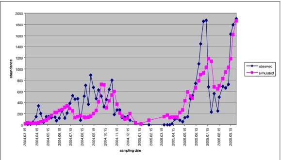
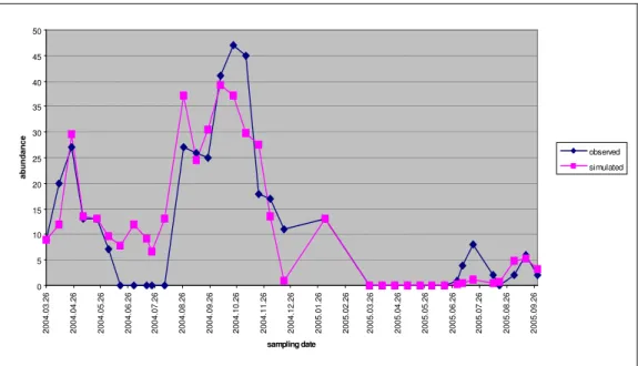
The four groups playing part in modelling, their observed and simulated patterns are presented in Figure4-Figure 7.

(15)

0 200 400 600 800 1000 1200 1400 1600 1800 2000

2004.03.15 2004.04.15 2004.05.15 2004.06.15 2004.07.15 2004.08.15 2004.09.15 2004.10.15 2004.11.15 2004.12.15 2005.01.15 2005.02.15 2005.03.15 2005.04.15 2005.05.15 2005.06.15 2005.07.15 2005.08.15 2005.09.15

sampling date

abundance

observed simulated

Figure 4.The observed and simulated individual numbers by cyclopoids during the survey.

0 50 100 150 200 250 300 350 400 450 500

2004.03.15 2004.04.15 2004.05.15 2004.06.15 2004.07.15 2004.08.15 2004.09.15 2004.10.15 2004.11.15 2004.12.15 2005.01.15 2005.02.15 2005.03.15 2005.04.15 2005.05.15 2005.06.15 2005.07.15 2005.08.15 2005.09.15

sampling date

abundance

observed simulated

Figure 5. The observed and simulated individual numbers by Eudiaptomus zachariasi during the survey.

(16)

0 5 10 15 20 25 30 35 40 45 50

2004.03.26 2004.04.26 2004.05.26 2004.06.26 2004.07.26 2004.08.26 2004.09.26 2004.10.26 2004.11.26 2004.12.26 2005.01.26 2005.02.26 2005.03.26 2005.04.26 2005.05.26 2005.06.26 2005.07.26 2005.08.26 2005.09.26

sampling date

abundance

observed simulated

Figure 6.The observed and simulated individual numbers by Ischnura pumilio during the survey.

0 500 1000 1500 2000 2500 3000

2004.03.15 2004.04.15 2004.05.15 2004.06.15 2004.07.15 2004.08.15 2004.09.15 2004.10.15 2004.11.15 2004.12.15 2005.01.15 2005.02.15 2005.03.15 2005.04.15 2005.05.15 2005.06.15 2005.07.15 2005.08.15 2005.09.15

sampling date

abundance

observed simulated

Figure 7. The observed and simulated individual numbers by phytoplankton during the survey.

Climate change scenarios, running the model with different scenario data series and historical data.

General Circulation Models (GCM) describe the physical process of the atmosphere, oceans and surface, providing an overall view from the prospective. These models supply data series with low resolution, which should be downscaled to the given region.

UKLO, UKHI and UKTR models were laboured in England. The first two models are

(17)

equilibrium scenarios, which estimate the meteorological parameters after setting the equlibrium, calculating with doubled carbon-dioxid level. In the names the LO and HI posterior constituents refer to the low and high resolution. The third scenario is a transient model, which is appropriate to making long-term predictions, and tracking the climate permanently. GFDL2535 and GFDL5564 GCM-s were developed in the United States. These models calculate with 1 per cent annual growth of carbon-dioxid concentration. In fine it is worth mentioning the BASE scenario, reckon with the present climate.

These scenarios were used up in our investigation. Data series were downscaled to the region of Debrecen, and specified for the period around 2050. Each data series of scenarios included 31 years, and also the historical data series included 31 years from 1960 to 1990. In this manner we got for each group, taking part in modelling, 31 predicted data series (daily abundance). The model was launched from the first January, excluding by Ischnura pumilio, the base individual number was 1 in each cases (modulating the base abundance is not really effecting the results).

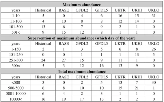
Testing the seasonal dynamics of cyclopoids on scenarios and historical data series Predictions were accepted until the day 330, as at the end of the year the abundance was overpredicted by some scenarios. In Table 3 we tried to summarize the results of modelling. Three aspects of predictions are displayed: the yearly maximum abundance, the supervention of the yearly maximum abundance, and the yearly total maximum abundance. The values of these three variables were divided into intervals, and the number of the years belonging to the intervals per scenarios, was given.

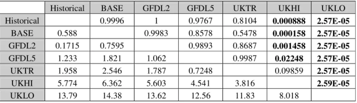
Based on Table 3, a transition can be seen: tending to UKHI and UKLO the maximum abundance is less, and the maximum abundance occurs sooner. A noticeable resemblance is between BASE-Historical data and GFDL2-GFDL5. UKLO seem to be discrete, with very low abundance (the maximum abundance is under 11 at each year).

Table 3.The results of the model for Cyclopoida running with the data series of scenarios and historical data series.

Maximum abundance

years Historical BASE GFDL2 GFDL5 UKTR UKHI UKLO

1-10 5 0 4 6 16 15 31

11-100 4 10 8 8 12 14 0

101-500 13 6 7 9 2 1 0

501< 9 15 12 8 1 1 0

Supervention of maximum abundance (which day of the year)

1-150 2 1 3 5 6 8 26

151-250 0 0 1 1 1 13 5

251-300 24 27 15 9 11 1 0

300< 5 3 12 16 13 9 0

Total maximum abundance

<500 3 0 2 5 13 7 30

500-5000 6 8 10 10 15 21 1

5001-10000 6 4 2 3 1 1 0

10000< 16 19 17 13 2 2 0

(18)

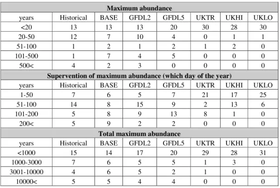
Testing the seasonal dynamics of Eudiaptomus zachariasi on scenarios and historical data series

Based on Table 4, we can make similar statements to the cyclopoids. The maximum abundance gradually decreases and it eventuates sooner tending to UKLO. The order of magnitude concerning the total individual numbers is pretty much the same. Noticeable similarity is between UKHI-UKLO-UKTR.

Table 4.The results of the model for Eudiaptomus zachariasi running with the data series of scenarios and historical data series.

<20 13 13 13 20 30 28 30

20-50 12 7 10 4 0 1 1

51-100 1 2 1 2 1 2 0

101-500 1 7 4 5 0 0 0

500< 4 2 3 0 0 0 0

1-50 7 6 5 7 21 17 25

51-100 14 8 15 9 2 13 6

101-200 5 8 9 13 8 1 0

200< 5 9 2 2 0 0 0

<1000 15 14 17 20 29 28 31

1000-3000 7 6 5 5 1 3 0

3001-10000 4 6 5 2 1 0 0

10000< 5 5 4 4 0 0 0

Testing the seasonal dynamics of Ischnura pumilio on scenarios and historical data series

Predictions were considered until the day 250 because of the high individual numbers (overprediction, like by the cyclopoids). According to Table 5, a reverse trend stands out as compared to the previous predictions, namely the maximum abundance increases and it occurs later. The previous transition can be noticed here as well, but it is the opposite, that is UKHI-UKLO is characterized by the highest individual numbers.

According to UKLO, the supervention of maximum abundance is not so different from BASE. The results of historical data-BASE and GFDL2535-GFDL5564 are similar, but UKHI and UKLO differ from each other. It is conspicuous when looking the supervention of maximum abundance, where GFDL2535 and GFDL5564 produced the same values, whereas UKHI and UKLO differ. It is worth paying attention to the high individual numbers in some cases (higher than by the zooplankton, whether above 5000).

(19)

Table 5.The results of the model for Ischnura pumilio running with the data series of scenarios and historical data series.

<100 30 26 18 12 19 14 7

100-1000 1 5 6 10 4 7 10

1001-5000 0 0 6 4 7 6 7

5000< 0 0 1 5 1 4 7

<150 14 15 2 2 4 4 1

150-200 2 3 0 0 0 1 13

201-225 4 7 5 5 4 3 11

226-250 11 6 24 24 23 23 6

<1000 29 25 15 8 16 12 5

1000-10000 2 5 5 11 7 6 8

10001-50000 0 1 9 7 7 8 6

50000< 0 0 2 5 1 4 12

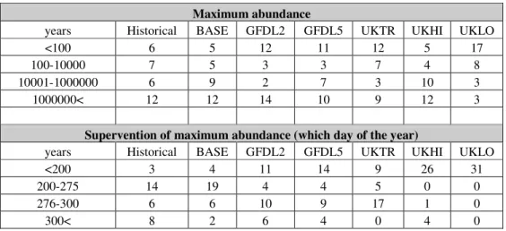
Testing the seasonal dynamics of phytoplankton on scenarios and historical data series In case of phytoplankton we left out the total maximum abundance from evaluation, as it often occured „algal blooms” with extreme high abundance while running the model. Based on Table 6, a transition is noticeable: tending to UKLO the maximum abundance occurs sooner and the maximum abundance is less. Latter is traceable chiefly by UKLO, while UKHI is similar to the historical results. The outcomes of BASE and historical data are similar.

Table 6.The results of the model for phytoplankton running with the data series of scenarios and historical data series.