Comparative Assessment of Climate Change Scenarios Based on Aquatic Food Web Modeling

Comparative Assessment of Climate Change Scenarios Based on Aquatic Food Web Modeling

Cs. Vadadi-Fülöp_&D. Türei_&Cs. Sipkay_&Cs. Verasztó_&

Á. Drégelyi-Kiss_&L. Hufnagel

Received: 25 October 2007 / Accepted: 28 May 2008

#Springer Science + Business Media B.V. 2008

Abstract In the years 2004 and 2005, we collected samples of phytoplankton, zooplankton, and macroinverte- brates in an artificial small pond in Budapest (Hungary).

We set up a simulation model predicting the abundances of the cyclopoids, Eudiaptomus zachariasi, and Ischnura pumilioby considering only temperature and the abundance of population of the previous day. Phytoplankton abun- dance was simulated by considering not only temperature but the abundances of the three mentioned groups. When we ran the model with the data series of internationally accepted climate change scenarios, the different outcomes were discussed. Comparative assessment of the alternative climate change scenarios was also carried out with statistical methods.

Keywords Hydrobiology . Community . Ecosystem . Climate change

1 Introduction

Climate change is one of the most crucial and influential ecological problem of our age; therefore, the number of investigations dealing with this problem is increasing permanently. It has several biological and nonbiological relations. Climate change and variability can influence aquatic ecosystems in a very sensitive way [32], so the research of the possible effects of climate change on aquatic ecosystems means an indispensable task. Applying climate change scenarios is one potential tool to evaluate the possible impacts of climate change. In this paper, we focus on the comparative assessment of climate change scenarios based on aquatic food web modeling. With this design, seasonal dynamics patterns will be described and simulated.

Predictable patterns of biodiversity often occur in freshwa- ter pelagic communities over yearly cycles in temperate regions of the globe [4]. It has been shown that abundance and structure of the zooplankton community display considerable variations on seasonal, interannual, and regional scales [1].

The objectives of this study were (1) the description of the phytoplankton, zooplankton, and macroinvertebrate assemblages in the examined pond, (2) the elaboration of a simple simulation model that is able to generate similar patterns to the observed ones, (3) the test of the model, (4) running of the model with the data series of different, internationally recognized climate change scenarios, sup- plying and interpreting of the predictions, and (5) compar- ative assessment of the alternative climate change scenarios with classical statistical methods.

We chose an artificial and small pond to examine, since it can be regarded as simpler and more closed than natural freshwaters, and the operation of the system could be easier to understand. The model generated simulated data based DOI 10.1007/s10666-008-9158-2

C. Vadadi-Fülöp (*)

:

:

Pázmány P. sétány 1/c, 1117 Budapest, Hungary e-mail: vadfulcsab@gmail.com C. Sipkay

:

Department of Mathematics and Informatics, Corvinus University of Budapest,

Villányi út 29–33, 1118 Budapest, Hungary Á. Drégelyi-Kiss

College of Technology of Budapest, Népszínház út 8,

1081 Budapest, Hungary

Cs. Vadadi-Fülöp (*)

I

I

Cs. Sipkay

I

on the daily mean temperature and population abundance of the previous day as inputs. We expected the model to indicate real patterns like the observed data series, and thus the climate change scenarios could be valued. By means of a simple simulation model, we were able to generate similar patterns like the observed one. When we ran the model with the data series of different climate change scenarios, we got a prospective notion of the abundance of the examined objects, which must be handled watchfully. The aim of the study is not the prediction but the comparative appreciation of the possible effects of the different, international climate change scenarios with the aid of a real model situation.

Present work is a methodological case study with emphasis on the new modeling methodology.

2 Review of Literature

2.1 Climate Change, Climate Change Scenarios

Climate change is alluded, when the fluctuation range of climatic elements shifts appreciably to higher or lower values, and this state remains for a long period [36].

Minnen et al. [22] introduced a new approach, the critical climate change, which is the quantitative magnitude of climate change above which unacceptable long-term effects on ecosystem may occur, according to current knowledge.

This method is capable to estimate quantitatively the vulnerability of natural ecosystems to environmental changes. The scientific results concerning climate change are summarized in Intergovernmental Panel of Climate Change reports.

Three types of scenarios are distinguished: synthetic, analogue, global climate model (GCM). General circulation models were developed at first to modeling the atmos- phere’s processes. Later, also the atmosphere’s interactions with the biosphere, hydrosphere, lithosphere, and cryo- sphere were taken into consideration, and these models were accounted as GCMs. Two types of GCMs are differentiated: equilibrium and transient models. The equilibrium model calculates with doubled level of carbon dioxide in the atmosphere. The model is run till it sets in an equilibrium state, namely a state when it evolves a stable temperature on the surface. By gradually increasing the level of carbon dioxide, transient models make it possible to determine the gradually changing climatic conditions [36]. The claim to apply GCMs for regional levels required the method of downscaling. The kernel of downscaling is considering the results of GCMs for great areas and setting statistical correspondence between the climatic variables of great and minor areas [36].

The climate change scenario can be defined as a likely combination of the change of climatic conditions, which

can be used for testing the possible effects and assessing the reactions for them [36]. According to [5], climate change scenarios are coherent, internally consistent, and plausible descriptions of possible future states of the world. These models are based on the simulations of general circulation models and regional climate models. Some remarkable institutes for developing GCMs are the undermentioned:

the Geophysical Fluid Dynamics Laboratory (GFDL), the Goddard Institute for Space Studies, the National Center for Atmospheric Research, and the UK Meteorological Office.

Scenarios are ambiguous, so it is rewarding and also common to use alternative scenarios in the studies.

Scenarios do not give factual forecasts, but they make hypothetical prospects. By all means, they are useful for biophysical and socioeconomic systems by giving the trend and amplitude of changes and the possible threshold values of processes that are sensitive to climate [36].

2.2 Seasonal Dynamics and the Modeling Approach with Special Regard to Climate Change

Seasonal and daily patterns of zooplankton populations are often predictable in natural lakes [4]. In Sommer’s opinion [29], seasonal succession of planctonic communities is driven by the changing availability of limiting resources to phytoplankton and zooplankton populations.

Christou [8] examined the abundance of copepods in a Mediterranean coastal area (Aegean Sea) during 5 years.

Copepod abundances and environmental parameters, almost all, exhibited pronounced annual cycles, and most copepods revealed repeated patterns and considerable interannual variability. Temperature and salinity were the most signif- icant environmental parameters accounting for the variabil- ity of abundances. The results of [10] suggest that in the Central Baltic Sea, the interannual variability of zooplank- ton species is controlled by the sea surface temperature during spring (significant correlation was found only in spring). The pattern of zooplankton productivity was changing over time in the subarctic Pacific, probably in response to interdecadal ocean climate variability [18].

These changes include two- to threefold shifts in total biomass, 30–60-day shifts in seasonal timing, and 10–25%

changes in average body length.

The first model dealing with the plankton succession (the so-called Plankton Ecological Group [PEG] model) was sketched just to 1986, as a result of the synthesis of many case studies [30]. The applicability of this model revealed that many types of lakes should be distinguished in the aspect of plankton, as the PEG-model is adapted only for modeling the plankton succession of the temperate, deep lakes.

Researchers working in 1970s, like [28], handled phyto- plankton as one variable and tried to explore the background

functions; though phytoplankton does not exist, it consists of many species evolved in different ways and is grouped in the way of community dynamics.

Such complex models set up in the 1960s were followed by simpler models [16]. The community approach was not detailed enough, and parametrization was set back by differentiating only seven functional groups [17].

Tilman [33] and Tilman et al. [34] showed a new way of laboring his source-allocation models, where certain popu- lation dynamics changes could be to interpreted. Namely, if we want to defend against algal bloom, we should know the main community dynamics beyond the autecological parameters of the given species.

The comparative works should be mentioned in the last decades that tried to contrast models set up for phytoplank- ton with those for terrestric communities. After many works, an approach was set up: A minor break in the weather, which is negligible for the offshore vegetation, can come up to a climate change for phytoplankton [31].

If we aim to examine the possible effect of climate change on aquatic communities, there are three approaches: moni- toring, experiment, and modeling. The advantage of applying models is that we have the chance to make predictions for the future period, which cannot be examined in the present time. Some former studies were run on the seasonal dynamics modeling of the macroinvertebrate community in Lake Balaton [25, 26], respectively, of macroinvertebrate species in artificial water bodies [35] and, moreover, zooplankton in the river Danube [27]. The abovementioned works were connected to climate change, as temperature- dependent simulation models were used to model the seasonal dynamics of the given species; what is more, data series of climate change scenarios were also applied.

3 Materials and Methods

3.1 Sampling Site

Sampling was conducted in an artificial small pond, located in Budapest (Hungary), in a yard of a family residence. The climate is temperate, and there is moderate shortage of rainfall. The mean yearly temperature is between 10.0 and 10.2°C [19]. The water surface was 522 dm², and the depth 30 cm. The bottom of the pond was formed by gravel and organic sediment. The water level was constant, there was no outflow, and the evaporated water was replaced with water from the tap. During the whole survey, neither treatment was applied, nor were plants removed. In winter, the pond was frozen up, but it has never frozen up to the bottom.

The plants, animals, and the sediment were introduced from a reach of Creek Szilas, opened up earlier with detailed examinations. Furthermore, different creatures

could colonize the pond from the air spreading passively or actively from the soil or air. The northern part of the pond and its three corners were covered with plants. Trees were not present in the vicinity. The following plants were characteristics of the pond: Iris pseudacorus, Carex acutiformis, Mentha aquatica, Myosotis palustris, Typha latifolia,Juncus effusus,Siumsp., andSparganiumsp.

3.2 Sampling Methods and Processing of Samples

The zooplankton sampling was conducted weekly from March 2004 to October 2005, except in winter, when sampling was more infrequent because of the low abun- dance. The sampling was representative, and samples were taken systematically from the whole water column. Twenty liters of water were filtered through a plankton net (17 cm diameter, 250 μm mesh size). The collected material was immediately handled with hot water; this treatment prevents the planktonic organism from contraction, making it easier to identify them later. Afterward, the sample was processed in a laboratory under a binocular microscope. Nauplii and Rotatoria were not determined. Identifying was performed to the closest taxa level. After sorting and counting, animals were preserved in formaldehyde, and some groups were identified later to the species level.

The macroinvertebrate sampling was performed biweek- ly from March 2004 to October 2005. Samples were taken from three locations. (1) Underlay: Collecting was con- ducted from three points of the pond (halfway and on the two ulterior brinks of the pond). Sampling was carried out with a pot fixed to a handle. During one bailing, the sediment and also water got into the pot. After sedimenta- tion, water was decanted partly, and the leftover was percolated. Percolation was carried out by using a sieve with small mesh size and also a strainer to avoid falling the rough detritus into the sample. (2) Water column: The spit was a strainer fixed to a long handle (1 mm mesh size).

Samples were taken from different points of the pond by six bailings. Plants getting into the strainer were poured into a basin. After bailings, part of the plants were leached with a water course (to the strainer). For other straining methods, see above. (3) Surface of the water: Animals observed on the surface were counted and estimated.

Pytoplankton was sampled by taking outxliters of water of the pond from different points (the volume was not deter- mined). With this, 4×50 cm³water was taken out and spun with an ultracentrifuge. Then, 4×5 cm³water was transferred into a vessel, and 3×1 drop from it was examined.

3.3 Simulation Methods and Statistical Analysis

For ecological modeling, discretely represented time and deterministic simulation approaches were applied in this

work. Abundance was given daily (discrete), and the outcome leads to the same result under the same conditions (deterministic). The predictions are valid only for the examined pond and at unchanged conditions (except temperature). The abundance of zooplankton andIschnura pumilio (Charpentier, 1825) was simulated by considering only temperature and their abundance at the previous day, whereas phytoplankton abundance was simulated by con- sidering temperature and the abundance of three other taxa (I. pumilio, Cyclopoida, Eudiaptomus zachariasi (Poppe, 1886)). Calculations were made with MS Excel and its Solver optimalizer program.

Tukey’s test was used to evaluate the results of the modeling. One-way analysis of variance and least signifi- cant difference could not be used because of the unequal variances. Scenarios and historical data series (see later) can be considered as treatments; therefore, we can make a comparison between them with the mentioned method. Our question was if there is any difference between the treatments. All data analyses were performed by using the PAST program [11].

3.4 Use of Concepts

(1) Climatic change scenario is a probable combination of the change of climatic conditions that can be used for testing the possible effects and estimating the reaction on these changes [36]. (2) Seasonal dynamics is the temporal change in the examined assemblage (change in abundance, species composition, or biomass), which is regulated by the temperature among others. (3) Simulation is the creating of artificial data series with mathematical models, which are reminiscent of data for temporal coenological state change.

(4) A simulation model is the formulating of hypothesis and conditions with mathematical methods concerning a tem- poral state change.

4 Results

Patterns of seasonal dynamics will be described by using a simulation model. In order to represent the seasonal dynamics of phytoplankton, we chose the whole phyto- plankton community since we thought it was competent for itself, and also we did not have the chance to identify taxa.

In the phytoplankton samples, there were also other groups not belonging to phytoplankton traditionally (Ciliata, Rotatoria, nauplius larvae, and some unidentified taxa);

however, these were also included in the model because of their role in the food web. Hereafter, we refer to this group as phytoplankton for simplicity. From the zooplankton community,E. zachariasi(frequentCalanoidaspecies) and

Cyclopoida were chosen for simulation modeling. Adults and copepodits were both comprised in the model. The dragonflyI. pumilio was a predominant species of macro- invertebrate assemblage; therefore, it seemed to be appro- priate for modeling its seasonal dynamics. We aimed to select the crucial taxa for modeling from different trophic positions, and the seasonal dynamics of the mentioned groups were described and simulated. The model system was run with the data series (mean daily temperature) of climate change scenarios as inputs.

The mathematical form is the following:

N_tþ1 ¼N_tR_t ð1Þ

where Nt+ 1 is the individual number of the population 1 day after time t, Nt is the individual number of the population at the time t, and Rt is the growth rate depending on the temperature.Rtis a mat function, which is created by fitting IF mat functions together (used in MS Excel). The occurring temperature values are divided into intervals, and each interval gets a value (parameters). In calculating the abundance, only the individual number of the previous day and one temperature parameter (it depends on the temperature at previous day) are consid- ered. Parameters were optimized with the Solver program of MS Excel in the following manner: The starting point was the first observed abundance value of the population.

Also, in the model, this was the first value, and in accordance with the form Eq. 1, the abundance of population was calculated for each day. The difference between the observed and generated values were comput- ed, squared, and then added, and finally, the sum of squares was minimalized (least squares fitting).

In the case of phytoplankton, the mathematical form is the following:

N_tþ1 ¼N_tR_tR_EudR_CycR_Isch ð2Þ whereNt+ 1is the individual number of the population 1 day after timet,Ntis the individual number of the population at the time t, Rt is the growth rate depending on the temperature, REud is the growth rate depending on the population of E. zachariasi, RCyc is the growth rate depending on the population of Cyclopoida, and RIsch is the growth rate depending on the population of I. pumilio.

In the case of the last three factors, the same optimization method was used for calculating their values.

Data series of mean daily temperature were used in the models as inputs. Meteorological data were supplied by the Hungarian Meteorological Office, measured in an observa- tion hut in Budapest Lőrinc, close to the pond.

The observed and simulated patterns of the investigated objects are presented in Fig. 1, 2, 3, and 4, whereas the parameters of the models are presented in Fig.5,6,7, and8.

4.1 Climate Change Scenarios, Running the Model with the Data Series of Different Scenarios and Historical Data

We used the data series of mean daily temperature specified for the period around 2050 (BASE, GFDL2535, GFDL5564, UKTR, UKHI, UKLO) on the basis of the results from the project CLIVARA [3, 12]. UKLO, UKHI, and UKTR models were labored in England. The first two models are equilibrium scenarios, which estimate the meteorological parameters after setting the equilibrium, calculating with doubled carbon dioxide level. In the names, the LO and HI posterior constituents refer to the low and high resolution.

The third scenario is a transient model that is appropriate to making long-term predictions and tracking the climate

permanently. GFDL2535 and GFDL5564 GCM-s are equi- librium models and were developed in the USA. These models calculate with 1% annual growth of carbon dioxide concentration. Finally, the BASE scenario is founded on the present climatic conditions. In addition, we employed the database of the project PRUDENCE [6], namely the A2 and B2 scenarios of the HadCM3 climate change model run by the Hadley Centre (HC) and the run results of the Max Planck Institute (MPI) for the A2 scenario. These data series are specified for the period of 2070–2100. All data series were downscaled for the region of Debrecen. Each data series of scenarios included 31 years, and also the historical data series included 31 years from 1960 to 1990.

In order to have an overall view of the scenarios applied in this study, we demonstrate the temperature changes

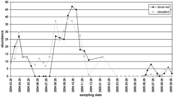
Fig. 2 The observed and simu- lated individual numbers byE.

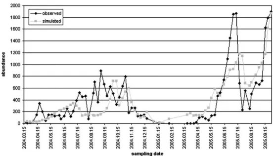
zachariasiduring the survey Fig. 1 The observed and simu- lated individual numbers by cyclopoids during the survey

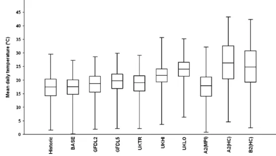
among scenarios in the form of mean daily temperature values. The results are presented in summer and winter terms since it is more reasonable to separate the data instead of looking at the changes in one block, particularly in the case of some scenarios. It is evident that the scenarios GFDL, UKTR, UKHI, UKLO, A2(HC), and B2(HC) forecast temperature rises while the A2(MPI) implies more temperate changes. A2(HC) and B2(HC) represent the highest temperature values, and at the same time, they are characterized by a wider amplitude (Fig.9). In the winter term, temperature values are less dispersed except UKHI, which has extreme low and high values as well (Fig.10).

A2(HC) and B2(HC) do not imply such remarkable changes as they were observed in the summer term. The differences between the scenarios are professed better in the summer term.

Since each data series of scenarios included 31 years, we got for each group, taking part in modeling, 31 predicted data series (daily abundance). The model was launched from the first January; excluding that byI. pumilio, the base individual number was 1 in each case (modulating the base abundance is not really affecting the results).

Predictions were accepted until day 330 by cyclopoids, as at the end of the year, the abundance was overpredicted by some scenarios. We tried to summarize the results in three aspects: the yearly maximum abundance, the day of abundance peak, and the yearly total abundance. According to UKHI, UKLO, A2(HC), and B2(HC) scenarios, which predict drastic global warming, the yearly maximum abundance and the yearly total abundance are less as compared to historical data, and the maximum abundance occurs sooner. A2(MPI) shows rather similar outcomes with

Fig. 4 The observed and simu- lated individual numbers by phytoplankton during the survey Fig. 3 The observed and simu- lated individual numbers byI.

pumilioduring the survey

UKTR, UKHI, and GFDL scenarios. A noticeable resem- blance is between BASE–historical data and GFDL2535–

GFDL5564. We can make similar statements for E.

zachariasiand for phytoplankton in most cases. Based on the results worked out forEudiaptomus, there is a noticeable similarity between UKHI–UKLO–UKTR scenarios, while UKHI is similar to the historical results by phytoplankton.

Predictions were considered until day 250 byI. pumilio because of the high individual numbers predicted in some cases. A reverse trend stands out as compared to the previous establishments; namely, the maximum abundance increases and the abundance peak occurs later by GFDL, UKTR, UKHI, and UKLO scenarios as compared with historical data and BASE. The scenarios A2(HC), B2(HC),

and A2(MPI) have similar outcomes with the run results of BASE and historical data. The results of historical data, BASE, and GFDL2535–GFDL5564 are similar, whereas UKHI and UKLO show some differences.

4.2 Statistical Analysis of the Results

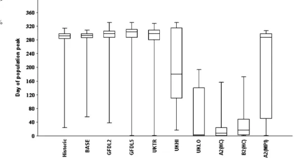
Hereinafter, we analyze the day of abundance peak occurring (the day of the year when the population peak is observed) among scenarios and historical results with statistical methods. We are interested in the statistical differences concerning temporal changes of population peak among scenarios and historical results. In order to detect any significant differences, Tukey’s pairwise com-

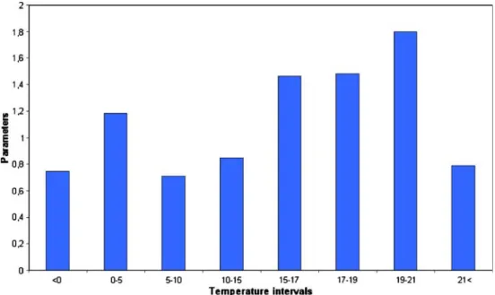
Fig. 6 The temperature param- eters of the model forE.

zachariasi

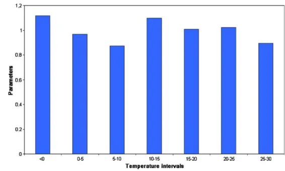
Fig. 5 The temperature parameters of the model for cyclopoids

parisons were performed including all scenarios and the historical results as well.

Figures11,12,13, and14show the characteristic features of abundance peaks. Each figure is based on 31 years per scenario. The results of Tukey’s pairwise comparisons are summarized in Table1.

Looking at the results of Cyclopoida, the scenarios UKHI, UKLO, A2(HC), B2(HC), and A2(MPI) indicate a remarkable shift in seasonal timing of population peak inasmuch as peaks are predicted to occur sooner. This trend is particularly true for the scenarios UKLO, A2(HC), and B2(HC). There are significant differences in several cases; A2(HC), B2(HC), and UKLO differ from historical results, BASE, GFDL, UKTR, and UKHI; furthermore,

UKHI and A2(MPI) show some differences from some scenarios.

The abundance peak of Eudiaptomusis shifting toward earlier by the scenarios UKTR, UKHI, UKLO, A2(HC), B2 (HC), and A2(MPI), which corresponds with the findings of Cyclopoida. A2(HC), B2(HC), and UKLO contrast signif- icantly with historical data, BASE and GFDL; UKHI and UKTR show similar outcomes, whereas A2(MPI) differs from BASE and UKLO.

The population of I. pumilio peaks later during the season according to the scenarios GFDL, UKTR, UKHI, and UKLO, while A2(HC), B2(HC), and A2(MPI) do not imply such remarkable trends, though they show some changes. The scenarios GFDL2535, GFDL5564, UKTR,

Fig. 8 The temperature parameters of the model for phytoplankton

Fig. 7 The temperature param- eters of the model forI. pumilio

UKHI, and UKLO proved to be different from BASE and historical data, whereas A2(HC) and B2(HC) were very similar to the latter group. However, A2(HC) and B2(HC) contrast significantly with GFDL, UKTR, UKHI, and UKLO. One more significant difference includes A2 (MPI)–GFDL5564.

Finally, algal population peaks follow the trend observed by the zooplankton community. A2(HC) and B2(HC) imply rather extreme seasonal patterns, with population peaks in the beginning of the year, although these abundances maxima lag behind with that of ordinary conditions. A2 (HC) and B2(HC) scenarios differ significantly from others but for UKLO. The latter scenario contrasts significantly with historical results, BASE, GFDL, and UKTR, and other significant differences include UKHI–historical data and A2(MPI)–UKLO.

After Tukey’s pairwise comparisons (Table 1), we can draw some general conclusions that are the following: (1) comparing historical data and BASE scenario, thepvalue is around 1, which is the evidence of the applicability of the scenarios; (2) GFDL2535 and GFDL5564 have very similar features (p=1 in almost every cases); (3) A2(HC) and B2 (HC) scenarios give the same payoff (p=1 in almost every cases); (4) A2(MPI) shows variable, discrete patterns.

5 Discussion

Our model is simplified as it considers only temperature and trophic connections (only by phytoplankton) to predicting the abundance. We have seen that the model predicted similar temporal patterns as compared to the Fig. 10 Box plot of the mean

daily temperature values by the historical data and scenarios (winter term).Linesrepresent the 10%, 25%, 50%, 75%, and 90% percentiles

Fig. 9 Box plot of the mean daily temperature values by the historical data and scenarios (summer term).Linesrepresent the 10%, 25%, 50%, 75%, and 90% percentiles

observed ones. Several authors draw our attention to the central regulatory role of temperature. According to [9], temperature is the most important factor regulating the temporal variance of mesozooplankton. Iguchi [13] and Dippner et al. [10] came into similar results. Temperature was in negative or positive correlation with almost all copepods abundances, and this correlation depended on the ecological habits of the species [8]. Long-term changes of many copepod species and other zooplankton groups have been also found to be related with changes in temperature and salinity [2, 21, 37]. According to [15], climatic conditions can influence interannual variation in macro- invertebrate populations, whereas cyclical patterns can be an expression of other factors.

McKee and Atkinson [20] examined the possible effect of climate change scenarios on populations of the mayfly

Cloeon dipterum and found that the temperature in itself does not have a significant influence on the abundance.

They supposed that temperature has indirect effects operating through interactions with predation and nutrient input. Peperzak [23] examined the effects of climate change on algae in the laboratory. He found that some species died, whereas others doubled their growth rates at a scenario with a 4°C temperature rise (for the year 2100). According to our former study [27] on Copepoda, we found that the maximum abundance of Cyclops vicinus occurs 1 to 1.5 months earlier as compared to the present conditions.

Christoffersen et al. [7] conducted experiments in artificial ponds to evaluate the potential effects of global warming on picoplankton and nanoplankton populations. Their results demonstrated that the direct effects of warming were far less important than the nutrient effect, and these variables

Fig. 12 Box plot of the popu- lation peak byE. zachariasiper scenario.Linesrepresent the 10%, 25%, 50%, 75%, and 90%

percentiles

Fig. 11 Box plot of the popula- tion peak by cyclopoids per scenario.Linesrepresent the 10%, 25%, 50%, 75%, and 90%

percentiles

displayed complex interaction. In our study, we also supposed that the temperature in itself does not have definitely an effect but can be related with other factors.

Our results show decreasing abundance by the scenarios calculating with global warming (excluding I. pumilio), which can be interpreted with the responsiveness to temperature change. Physiological reasons may be respon- sible for this phenomenon. Puelles et al. [24] found decreasing abundance by the zooplankton during 5 years, which was related to global warming.

Cyclopoid abundance decreases and the seasonal timing changes, insofar as maximum abundance occurs sooner among years. UKLO and UKHI scenarios predict drastic warming as they calculate with doubled level of carbon dioxide. The intense similarity of historical data and BASE is not strange, since the BASE scenario calculates with

contemporary climatic conditions. The discrete results of UKTR are attributable to the model, which is a transient one. The small differences between UKHI and UKLO can be attributed to their resolution. GFDL scenarios calculate with a low increase in the level of carbon dioxide;

therefore, these scenarios have an intermediate position between BASE and UKHI–UKLO. The A2 scenario forecasts more drastic changes in comparison with the B2 scenario [14]; even so, our results suggest minor difference between A2(HC) and B2(HC), whereas notable difference can be observed between the A2 scenarios of MPI and HC.

Concerning E. zachariasi, the former explanations are true here as well. In answer to global warming, their abundances decrease, and their abundance peak occurs sooner. The abundance of I. pumilio does not decrease but increases according to UKHI and UKLO scenarios, but A2 and B2 Fig. 14 Box plot of the popu-

lation peak by phytoplankton per scenario.Linesrepresent the 10%, 25%, 50%, 75%, and 90%

percentiles

Fig. 13 Box plot of the popu- lation peak byI. pumilioper scenario.Linesrepresent the 10%, 25%, 50%, 75%, and 90%

percentiles

scenarios do not imply such changes. In case of phyto- plankton, the effects of climate change is analogous with the pattern observed by the zooplankton community.

Our model is simplistic, as it takes only temperature and trophic connections into consideration in seasonal dynamics modeling. Other parameters such as light, oxygen conditions,

and nutrients were not measured; however, their effect might appear concealed. Predictions are simply informant and should be handled watchfully. The present work is a methodological case study, and we suppose that the presented model is only valid under unchanged conditions in the given artificial pond. In the future, other factors should also be Table 1 Summarized results of Tukey’s pairwise comparisons

Cyclopoida Eudiaptomus zachariasi Ischnura pumilio Phytoplankton

Hist–BASE

Hist–GFDL2 ***

Hist–GFDL5 ***

Hist–UKTR * *

Hist–UKHI ** ** ** **

Hist–UKLO *** *** * ***

Hist–A2(HC) *** *** ***

Hist–B2(HC) *** *** ***

Hist–A2(MPI) *

BASE–GFDL2 ***

BASE–GFDL5 ***

BASE–UKTR *** **

BASE–UKHI *** *** ***

BASE–UKLO *** *** ** ***

BASE–A2(HC) *** *** ***

BASE–B2(HC) *** *** ***

BASE–A2(MPI) ** ***

GFDL2–GFDL5 GFDL2–UKTR

GFDL2–UKHI **

GFDL2–UKLO *** *** ***

GFDL2–A2(HC) *** ** *** ***

GFDL2–B2(HC) *** ** *** ***

GFDL2–A2(MPI) GFDL5–UKTR

GFDL5–UKHI * *

GFDL5–UKLO *** *** **

GFDL5–A2(HC) *** *** *** ***

GFDL5–B2(HC) *** ** *** ***

GFDL5–A2(MPI) *

UKTR–UKHI

UKTR–UKLO *** ***

UKTR–A2(HC) *** *** ***

UKTR–B2(HC) *** *** ***

UKTR–A2(MPI)

UKHI–UKLO ***

UKHI–A2(HC) *** *** ***

UKHI–B2(HC) *** *** ***

UKHI–A2(MPI)

UKLO–A2(HC) **

UKLO–B2(HC) ***

UKLO–A2(MPI) *** * **

A2(HC)–B2(HC)

A2(HC)–A2(MPI) *** ***

B2(HC)–A2(MPI) *** ***

Significant differences are marked with asterisk.

*p<0.05, **p<0.01, ***p<0.001

included in the model. Such“simplified”systems are the basis of our better understanding of complex, natural ecosystems. In order to draw conclusions for larger-scale ecosystems under natural conditions, detailed, long-term databases are needed with additional factors. However, these field data are missing in most cases, partly due to the lack of time and some methodological difficulties.

Acknowledgments This investigation was supported by the projects NKFP 4/037/2001 and the OTKA T042583. The present paper is a contribution to the CLIVARA and PRUDENCE projects. Meteoro- logical data were provided by the Hungarian Meteorological Office.

Department of Systematic Zoology and Ecology, Eötvös Loránd University, and Department of Mathematics and Informatics, Corvinus University of Budapest, supported this research.

References

1. Arashkevich, E., Wassmann, P., Pasternak, A., & Riser, C. W.

(2002). Seasonal and spatial changes in biomass, structure, and development progress of the zooplankton community in the Barents Sea. Journal of Marine Systems, 38, 125–145. DOI 10.1016/S0924-7963(02)00173-2.

2. Baranovic, A., Solic, M., Vucetic, T., & Krstulovic, N. (1993).

Temporal fluctuations of zooplankton and bacteria in the middle Adriatic Sea. Marine Ecology Progress Series, 92, 65–75. DOI 10.3354/meps092065.

3. Barrow, E. M., Hulme, M., Semenov, M. A., & Brooks, R. J.

(2000). Climate change scenarios. In T. E. Downing, P. A. Harrison, R. E. Butterfield, & K. G. Lonsdale (Eds.), Climate change, climatic variability and agriculture in Europe: An integrated assessment(pp. 11–27). Oxford, UK: University of Oxford.

4. Bernot, R. J., Dodds, W. K., Quist, M. C., & Guy, C. S. (2004).

Spatial and temporal variability of zooplankton in a great plains reservoir. Hydrobiologia, 525, 101–112. DOI 10.1023/B:

HYDR.0000038857.19342.fd.

5. Carter, T. R., Parry, M. L., Harasawa, H., & Nishioka, S. (1994).

IPCC technical guidelines for assessing climate change impacts and adaptationp. 59. London: UCL/CGER.

6. Christensen, J. H. (2005).Prediction of regional scenarios and uncertainties for defining European climate change risks and effects. Final Report. p. 269. Copenhagen: DMI.

7. Christoffersen, K., Andersen, N., Sondergaard, M., & Liboriussen, L.

(2006). Implications of climate-enforced temperature increases on freshwater pico- and nanoplankton populations studied in artificial ponds during 16 months. Hydrobiologia, 560, 259–266. DOI 10.1007/s10750-005-12212.

8. Christou, E. D. (1998). Interannual variability of copepods in a Mediterranean coastal area (Saronikus Gulf, Aegean Sea).Journal of Marine Systems, 15, 523–532. DOI10.1016/S0924-7963(97) 00080-8.

9. Christou, E. D., & Moraitou-Apostolopoulou, M. (1995). Metab- olism and feeding of mesozooplankton at the eastern Mediterra- nean (Hellenic coastal waters).Marine Ecology Progress Series, 126, 39–48. DOI10.3354/meps126039.

10. Dippner, J. W., Kornilovs, G., & Sidrevics, L. (2000). Long-term variability of mesozooplankton in the Central Baltic Sea.Journal of Marine Systems,25, 23–31. DOI10.1016/S0924-7963(00)00006-3.

11. Hammer, O., Harper, D. A. T., & Ryan, P. D. (2001). PAST:

Paleontological statistics software package for education and data analysis.Paleontologia Electronica,4(1), 9.

12. Harrison, P. A., Butterfield, R. E., & Downing, T. E. (2000). The CLIVARA project: Study aims and methods. In T. E. Downing, P. A.

Harrison, R. E. Butterfield, & K. G. Lonsdale (Eds.), Climate change, climatic variability and agriculture in Europe: An integrated Assessment (pp. 3–10). Oxford, UK: University of Oxford.

13. Iguchi, N. (2004). Spatial/temporal variations in zooplankton biomass and ecological characteristics of major species in the southern part of the Japan Sea: A review.Progress in Oceanog- raphy,61, 213–225. DOI10.1016/j.pocean.2004.06.007.

14. IPCC (2007).Climate change 2007: The physical science basis.

Working group I contribution to the fourth assessment Report of the IPCC. Intergovernmental Panel on Climate Change. New York: Cambridge University Press.

15. Jackson, J. K., & Füreder, L. (2006). Long-term studies of freshwater macroinvertebrates: A review of the frequency, duration and ecological significance. Freshwater Biology, 51, 591–603. DOI10.1111/j.1365-2427.2006.01503.x.

16. Jorgensen, S. E. (1994). Fundamentals of ecological modeling (developments in environmental modeling 19) (2nd ed.). Amster- dam: Elsevier.

17. Jorgensen, E. S., & Padisák, J. (1996). Does the intermediate disturbance hypothesis comply with thermodynamics? Hydro- biologia,323, 9–21.

18. Mackas, D. L., & Tsuda, A. (1999). Mesozooplankton in the eastern and western subarctic Pacific: Community structure, seasonal life histories, and interannual variability.Progress in Oceanography,43, 335–363. DOI10.1016/S0079-6611(99)00012-9.

19. Marosi, S., & Somogyi, S. (1990). Magyarország kistájainak katasztere I–II. Budapest: MTA Földrajztudományi Kutatóintézet.

20. McKee, D., & Atkinson, D. (2000). The influence of climate change scenarios on population of the mayflyCloeon dipterum.

Hydrobiologia,441, 55–62. DOI10.1023/A:1017595223819.

21. Meise-Munns, C., Green, J., Ingham, M., & Mountain, D. (1990).

Interannual variability in the copepod populations of George Bank and the western Gulf of Maine.Marine Ecology Progress Series, 65, 225–232. DOI10.3354/meps065225.

22. Minnen, J. G., Onigkeit, O., & Alcamo, J. (2002). Critical climate change as an approach to assess climate change impacts in Europe: Development and application.Environmental Science &

Policy,5, 335–347. DOI10.1016/S1462-9011(02)00044-8.

23. Peperzak, L. (2003). Climate change and harmful algal blooms in the North Sea. Acta Oecologica, 24, 139–144. DOI 10.1016/

S1146-609X(03)00009-2.

24. Puelles, M. L. F., Pinot, J. M., & Valencia, J. (2003). Seasonal and interannual variability of zooplankton community in waters of Mallorca island (Baleric Sea, Western Mediterranean). 1994– 1999. Oceanologica Acta, 26, 673–686. DOI 10.1016/j.

oceact.2003.07.001.

25. Sipkay, Cs., & Hufnagel, L. (2006). Szezonális dinamikai folyama- tok egy balatoni makrogerinctelen együttesben. Acta Biologica Debrecina Supplementum Oecologica Hungarica,14, 211–222.

26. Sipkay, Cs., & Hufnagel, L. (2007). Klímaváltozási szcenáriók összehasonlító elemzése balatoni makrogerinctelen együttes alap- ján.Hidrológiai Közlöny,87, 117–119.

27. Sipkay, Cs., Nosek, J., Oertel, N., Vadadi-Fülöp, Cs., & Hufnagel, L. (2007). Klímaváltozási szcenáriók elemzése egy dunai Cope- poda faj szezonális dinamikájának modellezése alapján.Klíma 21.

Füzetek,49, 80–90.

28. Somlyódi, L., Herodek, S., & Fisher, F. (1983).Eutrophication of shallow lakes: Modeling and management. Luxemburg: IIASA.

29. Sommer, U. (1989). Plankton ecology: Succession in plankton communities. New York: Springer.

30. Sommer, U., Gliwicz, Z. M., Lampert, W., & Duncan, A. (1986).

The PEG-model of seasonal succession of planctonic events in freshwaters.Archiv fuer Hydrobiologie,106, 433–471.

31. Sommer, U., Padisák, J., Reynolds, C. S., & Juhász-Nagy, P.

(1993). Hutchinson’s heritage: The diversity–disturbance relation- ship in phytoplankton. Hydrobiologia, 249, 1–8. DOI10.1007/

BF00008837.

32. Straile, D. (2005). Food webs in lakes—Seasonal dynamics and the impacts of climate variability. In A. Belgrano, U. Scharler, J.

Dunne, & B. Ulanowitz (Eds.), Aquatic food webs: An ecosystem approach (pp. 41–50). Oxford, UK: Oxford Univer- sity Press.

33. Tilman, D. (1982).Resource competition and community struc- ture. Princeton: Princeton University Press.

34. Tilman, D., Kilham, S. S., & Kilham, D. (1982). Phytoplankton community ecology: The role of limiting nutrients.Annual Review

of Ecology and Systematics, 13, 349. DOI 10.1146/annurev.

es.13.110182.002025.

35. Vadadi-Fülöp, Cs., Sipkay, Cs., & Hufnagel, L. (2007). Klíma- változási szcenáriók értékelése egy szitakötőfaj (Ischnura pumilio Charpentier, 1825) szezonális dinamikája alapján.Acta Biologica Debrecina Supplementum Oecologica Hungarica,16, 211–219.

36. Varga-Haszonits, Z. (2003). Az éghajlatváltozás mezőgazdasági hatásának elemzése, éghajlati szcenáriók.AGRO-21.Füzetek,31, 9–27.

37. Viitasalo, M., Vuorinen, I., & Ranta, E. (1990). Changes in crustacean mesozooplankton and some environmental parameters in the Archipelago Sea (Northern Baltic) in 1976–1984.Ophelia, 31, 207–217.