ACCESS NuclearQuantumE ff ectsfromtheAnalysisofSmoothedTrajectories:PilotStudyforWater

Nuclear Quantum E ff ects from the Analysis of Smoothed Trajectories: Pilot Study for Water

Dénes Berta, Dávid Ferenc, Imre Bakó, and A ́ dám Madarász*

Cite This:J. Chem. Theory Comput.2020, 16, 3316−3334 Read Online

ACCESS

*

ABSTRACT: Nuclear quantum effects have significant contributions to thermodynamic quantities and structural properties; furthermore, very expensive methods are necessary for their accurate computation. In most calculations, these effects, for instance, zero-point energies, are simply neglected or only taken into account within the quantum harmonic oscillator approximation. Herein, we present a new method, Generalized Smoothed Trajectory Analysis, to determine nuclear quantum effects from molecular dynamics simulations. The broad applicability is demonstrated with the examples of a harmonic oscillator and different states of water. Ab initio molecular dynamics simulations have been performed for ideal gas up to the temperature of 5000 K. Classical molecular dynamics have been carried out for hexagonal ice, liquid water, and vapor at atmospheric pressure. With respect to the experimental heat capacity, our method outperforms previous calculations in the literature in a wide temperature range at lower computational cost than other alternatives. Dynamic and structural nuclear quantum effects of water are also discussed.

1. INTRODUCTION

Calculations of reaction free energy profiles and activation barriers are routinely performed within the rigid-rotor and harmonic-oscillator approximation;¹ meanwhile, the more accurate computation of thermodynamic quantities or vibra- tional spectra is still a great challenge.²⁻¹⁰ The inclusion of nuclear quantum effects (NQEs), such as zero-point energy (ZPE) or tunneling, is even more difficult.¹¹⁻¹³ Path-integral molecular dynamics (PIMD) and path integral Monte Carlo (PIMC) simulations are accurate, yet highly expensive methods to incorporate NQEs.^14,15 The computational cost of PIMD simulations can be significantly reduced by advanced techniques.¹⁶⁻¹⁸ Recently developed algorithms, such as a colored noise thermostat and quantum thermal bath, are more effective to add quantum effects to classical simulations,¹⁹⁻²¹ but settings need to be chosen carefully to prevent zero-point energy leakage.^22,23

When empirical water models were used in PIMD simulations, several properties deviated more from the experiments than in the classical simulations.²⁴⁻²⁷ In these quantum simulations, the liquid water becomes less structured and less viscous. This has been explained by double counting of quantum effects: once in the parameter optimization using experimental data, second in the quantum simulations. This is why several water models were reparametrized for accurate PIMD simulations resulting in q-SPC/Fw,²⁸q-TIP4P/f,²⁴and TIP4PQ/2005 models.²⁹ Another solution to avoid double counting is the application of PIMD with ab initio methods⁹or force fields trained on ab initio data.^25,27,30 Numerous methodological developments have also been made to calculate quantum free energy values from PIMD simulations.³¹⁻³⁵

In routine DFT calculations, with the optimized geometry in hand, the free energies are summed for all the different motions such as translation, rotation, and vibration, using the partition functions of the particle in the box, rigid rotor, and harmonic oscillator (RRHO) models.³⁶This approach works satisfactorily for small molecules at ambient temperatures, where the normal modes of vibrations can be considered as decoupled harmonic oscillators. For systems, where anharmo- nicity is significant, and/or the conformational space is extended, the RRHO fails to reproduce the exact thermody- namic quantities. Recognizing the need to address this issue, more sophisticated approaches use slightly modified partition functions on optimized geometries.^37,38 There are a few methods which can estimate quantum corrections from classical MD trajectories, for example, one- and two-phase thermodynamics methods (1PT, 2PT).³⁹⁻⁴¹In those cases the vibrational density of states (VDOS) is determined from molecular dynamics by the Fourier transformation of the velocity autocorrelation function. Quantum corrections are computed by the multiplication of VDOS with weight functions derived from the partition functions of motions. In the 1PT model, only vibrational modes are considered as harmonic oscillators; in the 2PT model, gas phase motions

Received: July 13, 2019 Published: April 8, 2020

Article pubs.acs.org/JCTC

License, which permits unrestricted use, distribution and reproduction in any medium, provided the author and source are cited.

Downloaded via 193.224.44.84 on September 28, 2020 at 11:19:18 (UTC). See https://pubs.acs.org/sharingguidelines for options on how to legitimately share published articles.

such as rotational and translational modes are also taken into account. The 2PT model is an improved method based on the original work of Berens et al. which corresponds to the 1PT method with anharmonic correction (1PT+AC).³⁹

The 2PT and 1PT+AC methods were successfully applied for the calculation of thermodynamic properties of several systems such as Lennard-Jonesfluids,⁴⁰water,^39,41−47organic liquids,^48,49 carbon dioxide,⁵⁰ adsorbed urea to cellulose,⁵¹ ionic liquids,^52,53carbohydrates,⁵⁴mixtures,⁵⁵and interfaces.⁵⁶ Heat capacity is generally used as a reference property for the benchmark of forcefields.42,48,49,53

The 1PT/2PT methods are still in continuous development in respect to accuracy and applicability.⁵⁷⁻⁶³

Here, we propose the Generalized Smoothed Trajectory Analysis (GSTA) method, which is numerically beneficial to the 1PT/2PT methods and, moreover, addresses their limitations arising from the used approximations. Our theory is demonstrated on the exact reproduction of heat capacity and internal energy of a harmonic oscillator. We have chosen different states of water as real-world examples as the heat capacity varies widely between phases, and it is still one of the most investigated materials in computations.⁶⁴ Beyond thermodynamic properties, structural and dynamic NQEs are also investigated.

2. THEORY

In a molecular dynamics simulations, the velocity autocorre- lation function (VACF) can be defined as follows:

t

v t v d

VACF( ) ( v ) ( )

2

∫ ^{τ τ τ}

=

+ ·

⟨ ⟩

−∞

+∞

(1) wherevis the velocity as a function of the time (t). Here, we refer to mass (m)-weighted VACF, but we assume identical masses in the derivations for simplicity. The vibrational density of states (VDOS) is the representation of the autocorrelation function (VACF) in the Fourier domain:

t t t t

VDOS( ) _t VACF( ) ( ) 2 VACF( ) cos(2 )d

∫

ν = { }ν = · πν

+∞

-

(2) where ν is the frequency. Since in our calculations real numbers are used, the Fourier cosine transform is applied.

Consequently, the VACF function is the inverse Fourier transform of the VDOS function:

t t t

VACF( ) VDOS( ) ( ) 2 VDOS( ) cos(2 )d

∫

ν ν πν ν

= _ν{ } = ·

+∞

-

(3) Usingt= 0, we get the norm of the VDOS function:

VDOS( ) (0) 2 VDOS( )d VACF(0) 1

∫

ν ν ν

{ } = =

=

ν

+∞

-

(4) Applyingν= 0 ineq 2, we get the norm of the VACF function:

t t t

VDOS(0) _t VACF( ) (0) 2 VACF( )d

∫

= { } =

- +∞

(5) Originally, Berens et al. proposed that quantum corrected density of states can be determined by the multiplication of VDOS with an appropriate weight functionw:³⁹

w

VDOS ( )^q ν =VDOS( ) ( )ν · ν (6) 2.1. Corrections of Vibrational Density of States (VDOS). 2.1.1. One-Phase Thermodynamics (1PT). In the 1PT method, only vibrational motions are considered. The internal energy is

U U d

U w

2 VDOS ( )

2 VDOS( ) ^U( )d

1PT 0

1 0

q

0 1

0

∫

∫

β ν ν

β ν ν ν

= +

= + ·

− ∞

− ∞

(7) where U₀ is the reference energy and β= (k_BT)⁻¹, k_Bis the Boltzmann constant, andT is the temperature.

The vibrational weight functionw^Ufor the energy originates from the quantum harmonic oscillator model:³⁶

w h h

( ) 2 coth 2

U ν β ν β ν

= i

kjjj y{zzz ₍₈₎

wherehis the Planck constant and coth denotes the hyperbolic cotangent function.

The heat capacity is the temperature derivative of the internal energy:

c U

T k Tw

2 VDOS( ) ( T( ))

V d

U

1PT 1PT

B

∫

= ∂

∂ = ·∂

∂

∞

(9) The last term in the integral is the weight function for the heat capacity:³⁶

w Tw

T h h

( ) ( ( )) h

exp( )

1 exp( )

c U 2

V ν ν

β ν β ν

= ∂ β ν

∂ =

− i

kjjjjj y

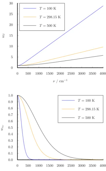
{zzzzz (10) The weight functions are shown inFigure 1. Using this weight functionw^cV(ν), the heat capacity can be obtained directly from the classical VDOS by integrating over the frequency domain:

c_V^1PT 2k_B VDOS( )w^c( )d

0

∫

= ·

∞

(11) In the classical limit (h→0), the 1PT method always givesk_B for the heat capacity, which corresponds to the classical harmonic value, so it cannot model anharmonicity.

2.1.2. Two-Phase Thermodynamics (2PT). Gas-like mo- tions such as translations and rotations are separated from vibrations in the 2PT method. The total VDOS is decomposed into vibrations, translations, and rotations:

VDOS( )ν =VDOS ( )_vib ν +VDOS ( )_trn ν +VDOS ( )_rot ν (12) Translation and rotation are determined for the center of mass and principal axes of the molecules, respectively.

Different weight functions are used for the different motions in the calculation of the thermodynamic properties:

c k w w

w

2 (VDOS ( ) ( ) VDOS ( ) ( ) VDOS ( ) ( ))d

V 2PT

B 0 vib vib trn trn

rot rot

∫

ν ν ν

= +

+

∞

(13) The weight function of translation and rotation is 1/2 for the heat capacity within the 2PT model.⁴¹

In the classical limit (h→0), the 2PT heat capacity can vary between k_B/2 and k_B per atom, not incorporating any anharmonicity, so the 2PT method cannot describe cases where the classical heat capacity is abovek_B. Another limitation

is that the molecular topology needs to remain the same during the simulation, so bond breaking/formation, thus chemical reactions, cannot be modeled. Moreover, intramolecular rotations cannot be described properly with 2PT.

2.1.3. 1PT with Anharmonic Correction (1PT+AC).Berens et al. proposed a quantum correction added to the classical heat capacities:³⁹

c_V^{1PT AC+} =c_V^cl+c_V^Δ (14)

The quantum correction can be determined from the quantum harmonic weight functionc_V^Δgiven by

c_V 2k_B VDOS( ) (w^c( ) 1)d

0

∫

= · −

Δ ∞

(15) If the integral terms are partitioned differently then we get:

c k w c

k c c

2 VDOS( ) ( )d

2 VDOS( )d

V

c

V

V V

1PT AC

B 0

cl

B 0

1PT AC

∫

∫

ν ν ν

ν ν

= · +

− = +

+ ∞

∞

(16) where the second term is the anharmonic correction. The 1PT +AC internal energy can be gained analogously as the heat capacity:

U^{1PT AC+} = U^1PT+U^{AC (17)}

where the anharmonic correction is the deviation of the classical internal energy (U^cl) from the ideal harmonic case:

U^AC=U^cl−β⁻¹ (18)

The 1PT+AC model always satisfies the correspondence principle in contrast with the 1PT or 2PT methods:

c c

lim

h V V

0

1PT AC cl

=

→ +

(19) This also implies that the technique is able to describe anharmonic motions to the extent of the method used to obtain the original classical trajectory.

2.2. Generalized Smoothed Trajectory Analysis (GSTA). In the previous sections, we briefly introduced the relevant methods from the literature about the correction of the VDOS function to get quantized thermodynamic proper- ties. In this section, we present a derivation to show that a similar correction can be performed in the time domain on the VACF function and on the coordinates.

2.2.1. Correction of Velocity Autocorrelation Function.

Convolution of two functionsfandgis defined as

f g t f t g

( ^∗ )( )⁼

∫

−∞

+∞

(20) is frequently used in digital processing for the smoothing of signals or thefiltering of high frequency noises.⁶⁵On the basis of the convolution theorem, the multiplication of the VDOS function with a weight function w is equivalent to a convolution of the Fourier transforms of the two functions.

The quantum corrected VACF function is the inverse Fourier transform of the quantum corrected VDOS function:

t t

w t w t

VACF ( ) VDOS ( ) ( )

VDOS( ) ( ) ( ) ( ( ) VACF)( )

q q ν

ν ν ν

= { }

= { · } = { } ∗

ν

ν ν

-

- -

(21) The Fourier transform of the weight function can be used for the quantum correction of the VACF function:

w ( ) ( ) ( )

γ τ =-_ν{ ν } τ ₍₂₂₎

From the corrected VACF function, the thermodynamic properties can also be calculated. For instance, the 1PT+AC heat capacity:

c_V^{1PT AC} 2k_B ^c( ) VACF( )d c_V

0

V AC

∫

= · +

+ +∞

(23) whereγ^cVis the Fourier transform of the weight function ineq 10according toeq 22.

h h h h

( ) 2

csch 2 2

coth 2

c 2 1

2 2 2 2

γ V τ π β

π β τ π

β τ π

β τ

= i −

kjjjj y {zzzzi

kjjjjj i

kjjjj y {zzzz y

{zzzzz (24) where csch is the hyperbolic cosecant function. The 1PT+AC internal energy takes the form

U^{1PT AC} U₀ 2 ¹ (w^U( ) ( ) VACF( )d U

0

∫

β ν τ τ τ

= + _ν{ } · +

+ − +∞

-

(25) and the weight function for VACF with the internal energy is given by

Figure 1.Weight functions for VDOS.

w h h

( ) ( ) ( ) 2

2 coth

2 cos(2 )d

U U

∫

γ τ ν τ β ν β ν

πντ ν

= _ν{ } = ·

- +∞ i

kjjj y{zzz

(26) The integral in eq 26 fails to converge as the w^U weight function increases monotonously. Fortunately, in real systems, the maximum frequency in the VDOS is alwaysfinite, so the weight function can be cut at a highfinite frequency with the application of an exponentially decreasing function:

exp bν

−| | i

kjjj y{zzz ₍₂₇₎

where variablebcontrols the exponential decay. The decay is faster as b increases. This function becomes unity as b approaches infinity:

lim exp b 1

b

−| |ν

=

→∞

i

kjjj y{zzz ₍₂₈₎

Theγ^Ufunction can be determined as a limit of an integral:

h h

( ) lim 2 b

2 coth

2 exp cos(2 )d

U

b

∫

γ τ β ν β ν ν

πντ ν

= −| |

·

→∞

+∞ i

kjjj y{zzz ikjjj y{zzz

(29) The integral can be evaluated in eq 29, and finally, the γ^U function can be expressed as a limit of a piecewise function:

h h

h ( ) lim

csch 2

coth 2

( )

U

0

2 2 2

2

γ τ

π β

π β τ τ π

β δ τ τ

=

− | | > |ϵ|

|ϵ| | | ≤ |ϵ|

ϵ→

l m ooooo oooo n ooooo oooo

i kjjjj y

{zzzz i

kjjjj y

{zzzz

(30) where δ denotes the dirac delta function. The norm of the function in eq 30 is 1. The coth function is the primitive integral of the csch²function. Since in the simulations the data are represented at discrete time intervalsΔt, it is useful to write theγ^Ufunction at discrete time steps in such a way that it is directly applicable for integration, i.e.,

( ) ( )

n t

n t n t

t

( )

coth ( 0.5) coth ( 0.5)

2

U

h h

2 ² 2 ²

γ Δ

=

+ Δ − − Δ

Δ

π β

π β

(31) where n is the index of the time step. When n = 0, the γ^U function takes the simple form:

t h t

(0) ( ) coth

U 1 2

γ π

= Δ ⁻ iβ Δ

kjjjj y

{zzzz

(32) The weight functions of VACF are shown inFigure 2.

2.2.2. Correction of Trajectory. The velocity autocorrela- tion function is actually a convolution function of the velocity with itself, i.e.,f= g= vin eq 20:

t v v t

VACF( ) ( v)( )

= ∗2

⟨ ⟩ (33)

According toeqs 1 and 2, the VDOS can be written in the form of:

v v t VDOS( ) _t ( v)( ) ( )

ν 2 ν

= { ∗ }

⟨ ⟩ -

(34)

Similarly, the quantum corrected counterpart can be written as v v t

VDOS ( )_{q t} ( v)( ) ( )

ν 2 ν

= { ̃ ∗ ̃ }

⟨ ⟩ -

(35) where ṽ is a modified velocity which satisfies eq 35. In the following steps, we determineṽ.

Substitutingeqs 34and35intoeq 6:

v v t v v t w

( )( ) ( ) ( )( ) ( ) ( )

t{ ̃ ∗ ̃ } ν = t{ ∗ } ν · ν

- - ₍₃₆₎

Using the convolution theorem:

v t v t w

(-_t{ ̃( )) ( ))} ν ² =(-_t{ ( )) ( ))} ν ²· ( )ν ₍₃₇₎ Assuming thatw(ν) is a non-negative real-valued function we get

v t( ) ( ) v t( ) ( ) w( )

t{ ̃ } ν = t{ } ν · ν

- - ₍₃₈₎

In the time domain, the multiplication byw(ν) is replaced by convolution.

v t( )̃ =(v∗-ν{ w( ) )( )ν } t ₍₃₉₎ g t( ):=-_ν{ w( ) ( )ν } t ₍₄₀₎ Thus, we arrived to a g(t) function whereby convoluting the velocities one can directly obtainṽand the quantum corrected vibrational density of states in eq 35. If one wants to use a general function, which can be applied any atomic velocity Figure 2.Weight functions for VACF.

function, then the vibrational weight function (eq 10) can be chosen:

g t w t

h ht

( ) ( ) ( ) sech 2

c c 2

2 2

v V ν π

β

π

= -_ν{ } = i β

kjjjj y {zzzz

(41) where sech means the hyperbolic secant function.

In the determination of a kernel function, the weight function of the internal energy can also be used:

g^U( )t = -_ν{ w^U( ) ( )ν } t ₍₄₂₎ Similarly to the determination of theγ^Ufunction ineq 26, the integral does not converge here either. We could not derive an analytic form for the Fourier transform ineq 42. In order to perform this Fourier transform numerically in a practical way, the weight function of the internal energy can be split into two parts:

w h h h

h h

( ) 2 coth

2 2

2 coth

2 1

U ν β ν β ν β ν

β ν β ν

= =

+ −

i kjjj y{zzz i

kjjjjj

j i

kjjj y{zzz y {zzzzz

z ₍₄₃₎

The Fourier transform of the second term in eq 43 can be readily evaluated numerically, while the Fourier transform of thefirst part can be determined analytically in a similar way as we did with theγ^Ufunction:

h t h

b t

2 ( ) lim

2 exp ( )

b

β ν β ν ν

= −| |

ν ν

→∞

-l -

moo

noo |

}oo

~oo l

moo

noo i

kjjj y{zzz| }oo

~oo ₍₄₄₎

The result can be given as a limit of a piecewise function:

h t

h

t t

h t

2 ( ) lim 1

4 2

1

2 ( )

0

β ν π 3

β

π

β δ τ

=

− | | | | > |ϵ|

|ϵ| | | ≤ |ϵ|

ν ϵ→

-l moo

noo |

}oo

~oo

l mooooo ooo n ooooo

ooo ₍₄₅₎

So theg^Ufunction can be calculated:

g t h h

h

t t

h t

( ) 2 coth

2 1

lim 1

4 2

1

2 ( )

U

0

3

β ν β ν

π β

π

β δ τ

= −

+

− | | | | > |ϵ|

|ϵ| | | ≤ |ϵ|

ν

ϵ→

- lm ooo

nooo i

kjjjjj

j i

kjjj y{zzz y {zzzzz z

|} ooo

~ooo l

mooooo ooo nooooo

ooo ₍₄₆₎

When the convolution is performed at discrete time step,Δt, the value of the kernel function in thenth step is

g n t h

t n n

t h h

n t

( ) 1

2 2

1 1/2

1 1/2

2 coth

2 1 ( )

U

π β

β ν β ν

Δ =

Δ | + | −

| − |

+ Δ -_ν − Δ

i

kjjjjj y

{zzzzz lm

ooo

nooo i

kjjjjj

j i

kjjj y{zzz y {zzzzz z

|} ooo

~ooo ₍₄₇₎

At zero time

g h

t t h h

(0) 1

2 2 coth

2 1 (0)

U

π

β β ν β ν

= Δ + Δ-_ν −

lm ooo

nooo i

kjjjjj

j i

kjjj y{zzz y {zzzzz z

|} ooo

~ooo (48) The kernels of g^U and g^cV are shown in Figure 3. g^U is represented in discrete points withΔt= 0.5 fs.

Utilizing a kernel function defined ineq 40, one can obtain filtered time-dependent variables such as coordinates, veloc- ities, and forces (x̃,ṽ,F̃):

x t( ):̃ =(x g t∗ )( ) ₍₄₉₎

v t x

t

x g t

x

t g v g t ( ): d

d

d( ) d

d

d ( )( )

̃ = ̃

= ∗

= ∗ = ∗

(50)

F t m v

t m v g

t m v

t g F g t ( ): d

d

d( ) d

d

d ( )( )

̃ = ̃

= ∗

= ∗ = ∗

(51) Having these variables smoothed, we are able to derive smoothed energy components. The smoothed kinetic energy (Ẽ_kin) can be obtained straightforwardly from smoothed velocities.

E ( , ):t 1mv

kin 2 η 2

̃ = ̃

(52) Figure 3.Kernels for trajectoryfiltration

2.2.3. Correction of Potential Energy.For the definition of the smoothed potential energy (Ẽ_pot), it can be expected to fulfill the following condition:

E

x F

d d

− pot

̃ ̃ = ̃

(53) The smoothed total energy is simply the sum of the smoothed kinetic and potential energies:

E_tot̃ =E_kiñ +E_pot̃ ₍₅₄₎ The kernel function can depend on several parameters like the temperature or the Planck constanth. In order to connect the classical systems with the quantum systems continuously, a fictitious η variable is introduced. η = 0 corresponds to the classical picture, andη=his the quantum one. Withη, we can perform an integration from the classical state to the quantum state.

It can be shown that the total energy remains conservative upon smoothing:

( )

E t

E t

E

t F x

t

mv t

Fv Fv 0

tot pot kin

1 2

∂ ̃ 2

∂ = ∂ ̃

∂ + ∂ ̃

∂ = − ̃∂ ̃

∂ +

∂ ̃

∂

= − ̃ ̃ + ̃ ̃ =

η η η

i kjjjj y

{zzzz i kjjjjj j

y {zzzzz z

i kjjjj y

{zzzz

(55) The total differential of the smoothed total energy is

E E

t t E E

E E E

x x

E F x

E

d d d d

d d d

d d d

t t

t t t t

t tot

tot tot tot

pot kin pot

kin kin

η η

η η

η η

η η

η η

η η

̃ = ∂ ̃

∂ + ∂ ̃

∂ = ∂ ̃

∂

= ∂ ̃

∂ + ∂ ̃

∂ = ∂ ̃

∂ ̃

∂ ̃

∂ + ̃ = − ̃ ∂ ̃

∂ + ̃

η

i kjjjj y

{zzzz i

kjjjj y

{zzzz i

kjjjj y {zzzz i

kjjjjj j

y {zzzzz z

i kjjjj y

{zzzz i

kjjjjj j

y {zzzzz z i kjjjj y

{zzzz i

kjjjj y {zzzz

(56) The negative of the first term can be called as work of smoothing:

F x

d : d

η t η Ω = ̃ ∂ ̃

∂ i kjjjj y

{zzzz

(57) The smoothed potential energy is defined at a specific time (t₀) as a correction on the original potential energy (E_pot) with the work of smoothing:

E ( )h _{t t} E _{t t} d ( )

h

t t

pot pot

0 0

∫

̃ | = | − Ω |

η η

= =

=

=

= (58)

Integrating this equation according to time yields the expectation value of smoothed potential energy:

E ( )h t E ( ) d ( , ) d

t h

pot

1

0 pot

∫

∫

⟨ ̃ ⟩ = − Ω

τ τ

η

− η

=

=

=

i =

kjjjj y

{zzzz (59) E_pot( )h E_pot( )h ( )h

⟨ ̃ ⟩ = ⟨ ⟩ − ⟨Ω ⟩ ₍₆₀₎

The average change of kinetic energy is equal to the average change of the potential energy (more details inAppendix A):

E_pot E_pot E_kin E_kin

⟨Ω⟩ = ⟨ ⟩ − ⟨ ̃ ⟩ = ⟨ ⟩ − ⟨ ̃ ⟩ ₍₆₁₎ So the mean smoothed total energy is

E_tot E_tot 2( E_kin E_kin )

⟨ ̃ ⟩ = ⟨ ⟩ − ⟨ ⟩ − ⟨ ̃ ⟩ (62)

Note that eq 62 corresponds to U^1PT+AC in eq 17. So we arrived to the same result as the 1PT+AC method, which is true for the heat capacity as well:

c_v^GSTA=c_v^{1PT AC+} (63)

Quantum-corrected state functions can be determined from the presented smoothed quantities, as shown by the example of heat capacity below.

3. COMPUTATIONAL DETAILS

3.1. Calculation of Heat Capacity. According to the Theory section, several estimators can be designed to determine the heat capacity depending on what is corrected:

VDOS, VACF, or the trajectory. The quantum correction can be introduced with different functions which correspond to the heat capacity or the internal energy, but the resulting thermodynamic functions can be transformed into each other by integration/differentiation. We used the kernel function of the heat capacity (eq 41) for the filtration since it is more convenient; i.e., its analytical form is known.

We performed several (50−120) independent NVE simulations around the T target temperature. The classical temperature (T_cl) was determined simply from the average classical kinetic energy for a particular trajectory:

T_cl= ⟨2 E_kin⟩/k_{B (64)}

The isochoric heat capacity can be determined from the slope of the mean total energies vsT_clfunctions:

c E

V T

V

cl tot

cl

= ∂⟨ ⟩

∂ i

kjjjjj y

{zzzzz ₍₆₅₎

c E

V T

V tot cl

= ∂⟨ ̃ ⟩

∂ i

kjjjjj y

{zzzzz

(66) The classic temperature originates from the classical normal- ization factor in eq 35. The isobaric heat capacity can be determined from the slope of the H vs T_cl (or H̃ vs T_cl) function:

c E pV

T

( )

p

p

cl tot

cl

= ∂ ⟨ + ⟩

∂ i

kjjjjj y

{zzzzz

(67)

c E pV

T

( )

p

p tot

cl

= ∂ ⟨ ̃ + ⟩

∂ i

kjjjjj y

{zzzzz

(68) For condensed phases,p= 1 atm was applied instead of the calculated average pressure because its fluctuation was larger than several hundred atm. We used linear regression to determine the heat capacities and their errors. The uncertainties of our calculations are given at the 95%

confidence level. Representative fittings are shown in the Supporting Information.

3.2. Born−Oppenheimer Molecular Dynamics Simu- lations.We carried out classical microcanonical normal mode sampling⁶⁶with Gaussian 09 Rev. E for the vibrations of one water molecule using B3PW91/6-311G(d,p) level of theory.^67,68 This functional was chosen since it reproduced the exact frequencies of a water molecule the most accurately with an average error of 6.1 cm⁻¹.⁶⁹ Initial energies were

distributed equally between modes according to the equipartition theorem. The equations of motion for the nuclear evolution were integrated employing the velocity Verlet algorithm with a 0.1 fs time step.⁷⁰ Then, 50 independent 1 ps long trajectories were generated around the desired temperature, and the total energies represented aχ² distribution.

3.3. Classical Molecular Dynamics Simulations.

Classical molecular dynamics simulations were performed with the Tinker molecular modeling software.⁷¹ The simulation box always contained 432 water molecules. For the liquid and vapor phases, a cubic box was applied. For Ih ice, water molecules were arranged according to the Bernal− Fowler ice rules⁷²having a vanishing net dipole moment.

First, we performed 10 ps long NpT simulations starting from previously equilibrated structures followed by 11 ps long NVE simulations. The last 1 ps data were used for the trajectory analysis. Here, 120 independent trajectories were generated to determine the heat capacity at a given temperature. In order to make the linearfitting more effective, the temperature of the thermostat was varied around the target temperature according to a χ²distribution. The equations of motion were integrated employing the Bussi−Parrinello algorithm⁷³ for the NpT ensemble and a modified Beeman algorithm⁷⁴for theNVEensemble with a 0.5 fs time step. In condensed phase simulations, the particle mesh Ewald (PME) method was applied for the long-range electrostatic interaction with 9.0 Å cutoff distance.⁷⁵ For the vapor phase, a larger cutoffof 113.0 Å was used with a 30×30×30 grid size for the Ewald summation.

We performed simulations for an NVT ensemble to determine the structural properties of the SPC/Fw water model at 298.15 K, with a simulation box size of 23.439 Å.

Then, 500 configurations were collected, and after 11 ps long NVEsimulations, the last 1 ps trajectory wasfiltered with the g^Ufunction withΔt= 0.1 fs to get onefiltered structure from each trajectory. These 500 independent structures were used to calculate the distributions of the intramolecular distances as well as the radial distribution functions.

For the calculation of the IR absorption spectrum of the AMOEBA14 water model, 120 independent NVEtrajectories were used. All simulations were 20 ps long, and they were equilibrated at 298.15 K before. We used a four term Blackman−Harris window before the Fourier transform of the dipole autocorrelation function.⁷⁶

3.4. Path Integral Molecular Dynamics Calculations.

PIMD simulations were carried out with AMBER12⁷⁷ in a canonical ensemble for 216 water molecules using the SPC/Fw model. The settings were taken from ref28, but 32 beads were used instead of 24. The length of the cubic simulation box was 18.68 Å, according to the equilibrium density. After 1 ns long equilibration, 1000 structures were collected for each bead in an additional 1 ns long simulation. For the calculation of the isochoric heat capacity, we performed canonical simulations at 288.15 and 308.15 K as well.

In order to determine the isobaric heat capacity for the liquid phase, NpT simulations were also performed at atmospheric pressure in the temperature range from 260.65 to 385.65 K.

4. RESULTS AND DISCUSSION

4.1. Harmonic Oscillator Model. Here, we show the effect of twofilters on the sum of two noncoupled oscillators at

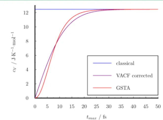
298.15 K. One oscillator has high frequency (3000 cm⁻¹), while the other has low frequency (100 cm⁻¹). The analytic curves are shown inFigure 4. Here,g^cVsmooths the vibration with high frequency, while g^U enhances the high frequency motion. The filtered function with g^U corresponds to the quantumfluctuation.

In the following section, we determine thefluctuation of the coordinates for a single harmonic oscillator. The time evolution of the position:

x t( )= Xcos(2πνt) (69)

whereXis the amplitude in a particular trajectory.

The probability distribution of the position for the harmonic oscillator in canonical ensemble:

x x

( ) 2 exp 2 βκ 2

π

ϱ = i−βκ

kjjj y

{zzz ₍₇₀₎

where κis the force constant of the harmonic potential. The filtered position is

x t x g t w X t

h h

x t

( ) ( )( ) ( ) cos(2 )

2 coth

2 ( )

U U ν πν

β ν β ν

̃ = ∗ =

= i

kjjj y{zzz

(71) The probability distribution of thefiltered position is given by

( ) ( )

( ) ( )

x x

x

( ) 1

coth 2 exp

2 coth

/2 coth

exp /2

coth

h h h h

h h h h

2 2 2 2

2

2 2 2 2

2

βκ π

βκ

κ π

κ

ϱ ̃ = − ̃

= − ̃

β ν β ν β ν β ν

ν β ν ν β ν

i

k jjjjj jjjjj jjjj

i

k jjjjj jjjjj jj

y

{ zzzzz zzzzz zz y

{ zzzzz zzzzz zzzz i

k jjjjj jjjj

y

{ zzzzz

zzzz (72)

This corresponds to the exact quantum fluctuation of the position for the harmonic oscillator. So the GSTA method is exact for the harmonic model for not only in the thermodynamic properties but for the coordinate distribution as well. This is a clear advance of GSTA compared to the 2PT method, since structural quantum effects cannot be inves- tigated with 2PT.

4.2. BOMD Simulations of One Water Molecule.Apart from cases where analytical solution exists, like a harmonic Figure 4.Filtration of the sum of two harmonic functions.

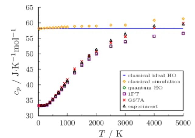
oscillator, we have chosen to test the proposed method on a single water molecule as a more realistic system. Born− Oppenheimer molecular dynamics (BOMD) simulations were carried out without rotation in the temperature range from 25 to 5000 K using the B3PW91 functional.⁶⁷The vibrational part of the isochoric heat capacity (c_V^vib) was obtained as the slope of the internal energy vs temperature function. For the sake of comparison, we estimated the isobaric heat capacity (including rotation and translation) based on these data asc_p=c_V^vib+ 1.5R + 1.5R+R=c_V^vib+ 4R.

We compare GSTA results with heat capacities determined using several different methods in Figure 5. The graph also

includes the ideal classical value, 7R = 58.2 J/K/mol (blue line) as well as the values determined with the application of the quantum harmonic oscillator model to the optimized geometry (green circles). At low temperature, all methods give very similar results, while at the higher temperature only the trajectory smoothing (red crosses) is close to the experimental values (black triangles).⁷⁸ This illustrates that anharmonicity can be described properly by GSTA in contrast with the quantum harmonic oscillator model or the 1PT method (purple squares).

4.3. Properties of Bulk Water.In order to demonstrate that our approach can work in very different circumstances, bulk water was considered as a test case in a wide temperature range. The quantum effects are decreasing while anharmonicity is increasing with temperature, and the heat capacity of water changes significantly from zero to 76.0 J/mol/K between different phases at atmospheric pressure.^79,80 The intra- molecular vibrations remain in the ground state at ambient temperature; therefore, many rigid water models are successful in reproducing the experimental values.^64,81 For the sake of generality, a flexible model is desired with which similar approaches can be examined even at high temperatures where excited vibrations can be populated as well. Three-site models are beneficial because analytical Hessian can be calculated for the optimized structures, which is not possible for polarizable water models. Considering these requirements, we have chosen the recently developed SPC/Fw⁸²water model which performs well on several physical properties.⁸¹ The parameters of the SPC/Fw water model were developed for classical molecular dynamics simulations to reproduce experimental data such as self-diffusion coefficient, dielectric constant, vibrational fre- quencies, oxygen−oxygen radial pair distribution function, and heat of evaporation.⁸²

4.3.1. Static Properties. Classical simulations cannot distinguish between the static properties of light and heavy water. In principle, exactly the same thermodynamic and structural properties should be determined for H₂O and D₂O since classical statistical thermodynamics predicts that equilibrium properties (heat capacity, molar density, surface tension, etc.) are independent of the masses of atoms. To reveal the different NQEs of classical trajectories, we need post processing methods like 1PT, 2PT, 1PT+AC, or GSTA. An important issue is to decide the reference which the computed quantities are compared to. Converged PIMD simulations provide exact static properties within the limit of the particular water model. However, empirical potentials are developed to reproduce various experimental data with classical simulations.

Thus, our strategy is to compare the different approximate values to both PIMD results and experiments as well.

Heat Capacity.At a given temperature, we determined the isobaric heat capacity as the derivative of the enthalpy vs temperature function from 120 independent 1 ps micro- canonical trajectories. Three states such as Ih ice, liquid water, and vapor were simulated at temperatures from 25 to 1000 K at atmospheric pressure (Figure 6). The classical ideal values are also shown with blue lines for the condensed and vapor phases in thefigure (9R= 74.8 J/K/mol, 7R= 58.2 J/K/mol, respectively).

The nuclear motions can be accurately described by independent harmonic oscillators at low temperature; there- fore, the heat capacity can be estimated quite well with all methods in the case of hexagonal ice (black triangles inFigure 6). Our method (denoted with red crosses) also gives values close to the experimental ones.⁷⁹ The maximum deviation is 6.0 J/mol/K atT = 200 K, probably due to the fact that the SPC/Fw water model was developed for liquid water and not for ice. A typical indication of this is that the melting point of the SPC/Fw water model is similar to that of the SPC/E water model (215 K), well below the experimental value (273.15 K).⁸³

For liquid water, the harmonic oscillator model is qualitatively wrong as it fails to describe anharmonicity captured already by classical simulations (yellow diamonds in Figure 6). The smoothing correction successfully takes the coupled motions of the molecules into account, thus performing outstandingly when compared to the experimental values. The isobaric heat capacity calculated by PIMD is somewhat higher (green circles inFigure 6). Most importantly, Figure 5.Isobaric heat capacities of a single water molecule from

BOMD simulations.

Figure 6.Isobaric heat capacities of bulk water in different phases.

GSTA performs much better than the classical model or the 1PT method no matter what reference we use, i.e., experimental value or PIMD results. Intramolecular vibrations arefiltered out in theg^cV-smoothed trajectories. In this aspect, water molecules behave rigidly in these liquid simulations (see the animation in theSupporting Information). This is in line with the experience that the overall performance of rigid water models is comparable to that of the flexible ones at room temperature.^64,81

For the vapor phase, we used the same water model and trajectory analysis as in condensed phases (Figure 6). GSTA gives reasonable results but overestimates the experimental heat capacities by about 3.2 J/mol/K. This is probably due to the fact that the dipole moment of the SPC/Fw water model is adjusted to liquid properties and considering that it is high compared to the dipole moment of a single water molecule in the gas phase (2.39 vs 1.85 D, respectively). The 1PT method overestimates the experimental values with 16 J/mol/K as a consequence that it considers only harmonic vibrations.

Overall, the smoothed SPC/Fw simulations are able to reproduce the heat capacity with an average error of 3.1 J/mol/

K in an extended temperature range at atmospheric pressure.

We have found two computational studies in the literature which investigated the heat capacities of the three most important phases of water. Yeh et al. used the 2PT method with different rigid water models, and all calculated heat capacities deviated more than 6.7 J/mol/K from the experi- ments.⁴⁵Shinoda and Shiga performed PIMD simulations for the three phases using theflexible SPC/F water model.⁸⁴They reproduced the experimental values excellently for ice and gas phase, but the heat capacity of liquid water was significantly underestimated by 16.6 J/mol/K.

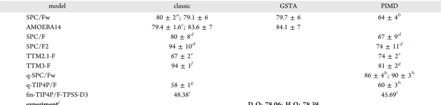
We have investigated other water models to examine their performance for the calculated heat capacities of liquid water (atT= 298.15 K,p= 1 atm). Besides the discussed SPC/Fw model, other potentials were also tested including rigid, polarizable, and four-site models.Table 1includes results from previous works as well for comparison. Regarding the classical heat capacities (c_p^cl), we have reproduced the literature data with small differences, which validates our simulations. GSTA- corrected heat capacities vary between 72.8 and 80.9 J/mol/K with the different water models around the experimental value.

The 1PT and 2PT methods give values from 52.2 to 86.6 J/

mol/K, and generally, rigid models perform better. The PIMD heat capacities range from 58.2 to 92.8 J/mol/K. The PIMD values can be considered as the exact heat capacity for a particular water model. Previously, the PIMD heat capacity of the SPC/Fw water model was found to be 88.7 J/mol/K, significantly higher than that of the experimental (75.4 J/mol/

K) or the GSTA values (72.8 J/mol/K). In our PIMD simulations on anNpTensemble, the isobaric heat capacity is 79.6 J/mol/K. In order to resolve this contradiction, we performed PIMD simulations on a canonical ensemble with the same settings as in the literature.²⁸Using the same number of beads, 24, we obtain 79.8 J/mol/K for the heat capacity, but with 32 beads it decreases to 76.6 J/mol/K. This indicates that there is a discrepancy between the value obtained here and those from earlier simulations. Still, we note that our PIMD heat capacity is in reasonable agreement with the experimental and the GSTA values. Our results indicate that the SPC/Fw water model reproduces the experimental heat capacity sufficiently. On the basis of the comparisons discussed here, we conclude that GSTA is an accurate and robust method in

the sense that the calculated heat capacities are less sensitive to the chosen potential.

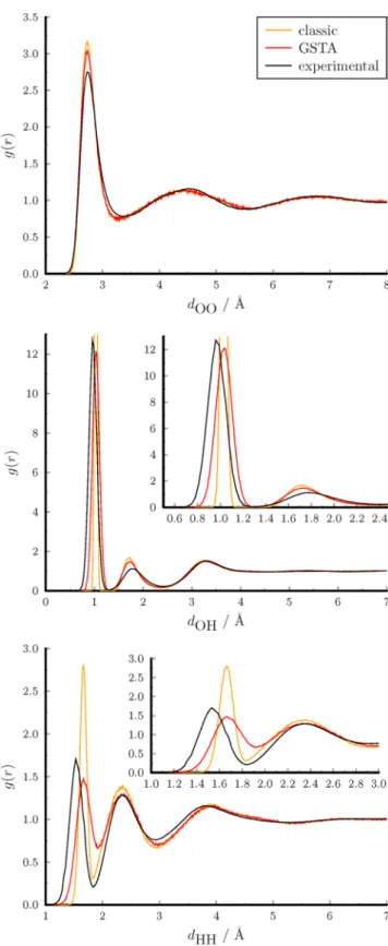
Structure of Liquid Water.A quantum-corrected structure can be obtained after thefiltration of the coordinates with the kernel function of the energy (g^U). The largest NQE in the structural properties of water is the quantumfluctuation of the hydrogen atoms. This effect is illustrated in the distribution of the intramolecular distances in Figure 7 and also in the animation (Supporting Information). The distribution deter- mined from PIMD simulations can be considered as the exact reference. The distributions of the intramolecular distances become broader compared to the classic results according to the Heisenberg uncertainty principle. The classical distribu- tions are too narrow, but the average distances are almost identical (Table 2). The GSTA method reproduces almost perfectly the exact distributions with a slight shift of 0.01 Å for the maxima.

The classical and thefiltered radial distribution functions are shown inFigure 8together with the experimental data.⁹¹The positions of the classical peaks are not altered significantly by thefiltration, but they become broadened and get closer to the experimental curves. Note that the 1PT and 2PT methods do not correct the structural properties.

Table 1. Calculated Isobaric Heat Capacities of Liquid Water^a

potential flexibility c_p c_p^cl

experiment 75.4 −

1PT or 1PT+AC

AMOEBA14 flexible 85.7^b 110.6^b

F3C flexible 84.5^c,r 109.6^c,r

SPC/E flexible 86.6^d,r 123.7^d,r

WATTS flexible 72.5^e,r 107.3^e,r

SPC/E rigid 73.0^d,r 87.4^d,r

2PT

AIMD−PBE flexible 52.2^f,r 90.1^f,r

F3C flexible 67.4^f,r 104.6^f,r

ReaxFF flexible 73.0^f,r 108.4^f,r

SPC-Fw flexible 69.3^f,r 109.5^f,r

SPC/E rigid 76.7^f,r; 68^g 87.3^f,r; 87^g TIP3P rigid 58.3^f,r; 60^g 67.5^f,r; 86^g TIP4P/2005 rigid 77.5^f,r; 68^g 85.5^f,r; 89^g TIP4P-Ew rigid 69.0^f,r; 69^g 80.8^f,r; 86^g

PIMD

SPC/F flexible 59.0^h,r 117.2^h,r

SPC/F2 flexible 58.2^i,r 117.2^i,r

SPC-Fw flexible 88.7^j,r; 79.6±0.5 113.8^j,r

q-SPC/Fw flexible 92.8^j,r −

q-TIP4P/F flexible 66.7^k,r −

TIP4PQ/2005 rigid 75.3^l −

GSTA

AMOEBA14^b flexible 80.9±0.7 113.5±0.6

F3C^c flexible 76.3±0.7 108.4±0.5

SPC-Fw^m flexible 72.8±0.6 109.3±0.4

TIP3Fⁿ flexible 72.8±0.7 106.9±0.6

TIP4P/2005F^o flexible 80.1±0.9 113.4±0.7

TIP3P^p rigid 75.0±1.0 81.2±0.9

TIP4P/2005^q rigid 79.0±0.7 87.1±0.6

aT= 298.15 K,p= 1 atm; all values are given in J/mol/K.^bref42.^cref 43.^dref44.^eref39; 2PT.^fref46.^gref45; PIMD.^href84.ⁱref85.^jref 28.^kref26.^lref86; GSTA: this work.^mref82.ⁿref87.^oref88.^pref89.

qref90.^rc_pwas estimated from the givenc_Vasc_p=c_V+ 0.8 J/mol/K.

Static Dielectric Constant.The static dielectric constant is another equilibrium property which exhibits nuclear quantum effects. Although, for liquid water the effect of deuterium substitution is small, the experimental dielectric constants are 78.39 vs 78.06 for H₂O and D₂O;⁹²in ice, the isotope effect is the opposite and more enhanced. The static dielectric constants of ordinary and heavy ice are 110 and 124 parallel to thecaxis of the crystal at−25°C, and the difference is even larger at lower temperature.

We have calculated the dielectric constant for both the classical andfiltered structures at 298.15 K using the following relationship:

V M M

1 4

3 ( )

s

0

2 2

ϵ = + πβ

ϵ ⟨ ⟩ − ⟨ ⟩

(73)

where ϵ0 is the vacuum permittivity,V is the volume of the simulation box, and M is the total dipole moment of the system. We computed the dielectric constant for SPC/Fw and AMOEBA14 water models. InTable 3, we collected our GSTA results along with previous classic and PIMD values from the Figure 7. Probability distribution functions of intramolecular

distances.

Table 2. Intramolecular Distances of Bulk Water

OH distance/Å

classic GSTA PIMD

mean 1.03 1.04 1.03

standard deviation 0.03 0.07 0.07

HH distance/Å

classic GSTA PIMD

mean 1.66 1.68 1.66

standard deviation 0.06 0.12 0.12

Figure 8.Radial distribution functions of atom pairs in liquid water.