An Approach to Modeling Closed-Loop Kinematic Chain Mechanisms, Applied to Simulations of the da Vinci Surgical System
Radian A Gondokaryono
1†, Ankur Agrawal
1†, Adnan Munawar
1, Christopher J Nycz
1, and Gregory S Fischer
11Robotics Engineering Department, 85 Prescott St, Worcester, MA, USA, 01609
†These authors contributed equally to this work
ragondokaryono@wpi.edu, asagrawal@wpi.edu, amunawar@wpi.edu, cjnycz@wpi.edu, gfischer@wpi.edu
Abstract: Open-sourced kinematic models of the da Vinci Surgical System have previously been developed using serial chains for forward and inverse kinematics. However, these models do not describe the motion of every link in the closed-loop mechanism of the da Vinci manipulators; knowing the kinematics of all components in motion is essential for the foundation of modeling the system dynamics and implementing representative simulations.
This paper proposes a modeling method of the closed-loop kinematics, using the existing da Vinci kinematics and an optical motion capture link length calibration. Resulting link lengths and DH parameters are presented and used as the basis for ROS-based simulation models. The models were simulated in RViz visualization simulation and Gazebo dynamics simulation. Additionally, the closed-loop kinematic chain was verified by comparing the remote center of motion location of simulation with the hardware. Furthermore, the dynamic simulation resulted in satisfactory joint stability and performance. All models and simulations are provided as an open-source package.
Keywords: Surgical Robots; Closed Chain Model; Kinematic Calibration; ROS Simulations
1 Introduction
Advances in the field of medical robotics have enabled the commercial success of tele-operated surgical robots in medical practice. Among these robots, the Intuitive Surgical’s da Vinci is the most recognized system in the market [1].
Although there are a number of different models and configurations, the da Vinci, Figure 1, typically comprises of three slave Patient Side Manipulators (PSMs), one slave Endoscope Camera Manipulator (ECM), a passive Setup Joint (SUJ)
Cart and two Master Tool Manipulators (MTMs). The SUJ Cart is used to position the PSM and ECM manipulators in the desired configuration with respect to the patient before the surgical procedure [2]. The manipulators’ tool is inserted through a trocar which is placed through the incision of the patient. The surgeon then controls the movement of these tools using the MTMs.
The success of the da Vinci in clinical practice has sparked significant research efforts worldwide to augment the currently available functionality. For example, adding haptic sensing to restore tactile feel [3], automating camera control to reduce the effort of operation [4], and adding an assistive control to increase the safety of the system [5]. Robot-assisted surgery using da Vinci involves many challenging subtasks. One of the more challenging subtasks is suturing and is an active research topic in terms of automation [6].
To accommodate this expanding research related to novel algorithms, John Hopkins University and Worcester Polytechnic Institute have developed software and firmware in conjunction with hardware [7] [8] to access low-level control data of the PSMs, ECM, and MTMs. The da Vinci robot, the open-source hardware robot controllers, and the open-source software/firmware is called the da Vinci Research Kit (dVRK).
Among the open-source applications, the dVRK community has also provided kinematic models of the PSMs, ECM, and MTMs (https://github.com/WPI- AIM/dvrk-ros) which visualizes the hardware components. These models correspond to the dVRK forward kinematics used for position control which represents each manipulator as a serial chain. This is done by simplification of the remote center of motion (RCM) in Figure 2 where the double four-bar linkage (yellow, orange, and pink lines) is represented as one joint with an axis of rotation at the RCM. An RCM is a fixed virtual point in space constructed by two intersecting rotation axis of the first and second joints.
While suited for real-time kinematic applications, this simplification does not accurately describe the motion of every link which is used as a foundation for describing the dynamics of the manipulators. Essentially, dynamics are necessary for a variety of applications including model-based control [9], gravity compensation [10] and representative simulations [11].
Most da Vinci simulations such as dV-Trainer [12] and Robotic Surgery Simulator (RoSS) [13] are used for training surgeons [14]. Research on the objective criteria of these simulations has been done, for example, on the force/torque evaluation of surgical skills in minimally invasive surgery [15]. Many research examples on haptics and force feedback [16] of the System suggests that accurate kinematics and dynamics should be an essential feature of a simulation. Such a simulation of the da Vinci has been developed in V-REP for research of novel control algorithms in [11].
This paper presents the procedure to obtain closed-loop kinematic chain models of the da Vinci Surgical System. Models were first developed using the dVRK forward kinematics. Next, a motion capture system with least squares axis calibration method is used for obtaining the missing data of the double four-bar linkage. To provide a useful application, the models are simulated in Robot Operating Systems [17] (ROS) visualization tool namely RViz [18], and Gazebo.
Gazebo uses physics engines to simulate dynamics [19]. While RViz currently only supports serial chains, it is possible to add closed-loop kinematic chains in Gazebo [20]. The simulated RCM of the models is then verified with the physical RCM of the hardware using a least squares calibration of the tool-tip obtained via motion capture system. The presented models and the simulations are available as an open-source package at https://github.com/WPI-AIM/dvrk_env.
Figure 1
The da Vinci Surgical System simulated in RViz
2 Kinematic Modeling
Figure 1 shows the daVinci surgical system divided into main components: a Setup Joint (SUJ) Cart, three passive SUJ-PSM 6 degree-of-freedom (DOF) arms, one passive SUJ-ECM 4 DOF arm, three PSMs, one ECM, and two MTMs.
The kinematics of the SUJ Cart, SUJ-PSM, and SUJ-ECM were readily available in the dVRK repository [6] and are explained here for an understanding of the
CAD/Simulation model development in Section 3. The serial chain kinematics of the PSM, and ECM in the dVRK repository are used for manipulator Cartesian position control of the dVRK. Therefore, our close-loop kinematic chain models correspond to the dVRK repository serial chain kinematic models. The missing closed-loop kinematic chain parameters are obtained with an optical motion capture axis distance calibration method explained in Section 2.4. The following sub-sections explain the developed kinematic models utilizing modified Denavit- Hartenberg (DH) convention.
2.1 Setup Joint Cart
The SUJ-PSM arms have 6 DOF each described by a vertical prismatic joint, four vertical revolute joints, and a horizontal revolute joint. Table 1 describes the modified DH parameters for the identical SUJ-PSM1 and SUJ-PSM2 arms. Table 2 describes the SUJ-PSM3 arm which has similar kinematics to SUJ-PSM1, 2, but different lengths. Table 3 describes the SUJ-ECM which is similar to SUJ-PSM until the last vertical revolute joint at which the ECM is mounted at a 45-degree angle.
Figure 2
Set Up Joint (SUJ) Cart kinematics and frame definitions shown in Rviz 6
Table 1
SUJ-PSM1, 2 modified DH parameters
Link Joint ai [m] αi [rad] di [m] θi [rad]
1 P 0.0896 0 q1 0
2 R 0 0 0.4166 q2
3 R 0.4318 0 0.1429 q3
4 R 0.4318 0 -0.1302 q4 + π/2
5 R 0 π/2 0.4089 q5
6 R 0 -π/2 -0.1029 q6 - π/2
Table 2
SUJ-PSM3 modified DH parameters
Link Joint ai [m] αi [rad] di [m] θi [rad]
1 P 0.0896 0 q1 0
2 R 0 0 0.3404 q2
3 R 0.5842 0 0.1429 q3
4 R 0.4318 0 0.2571 q4 + π/2
5 R 0 π/2 0.4089 q5
6 R 0 -π/2 -0.1029 q6 - π/2
Table 3
SUJ-ECM modified DH parameters
Link Joint ai [m] αi [rad] di [m] θi [rad]
1 P 0.0896 0 q1 0
2 R 0 0 0.4166 q2
3 R 0.4318 0 0.1429 q3
4 R 0.4318 0 -0.3459 q4 + π/2
5 R 0 -0.7853 0 π/2
6 R -0.0667 0 0 0
7 R 0 0 0.1029 π/2
2.2 Patient Side Manipulator
The PSM kinematics and associated frame definitions are described in Figure 3.
Following the modified DH convention, the axis of rotation (translation for prismatic joints), q, of each frame corresponds to the z-axis (blue). Positive rotation is counterclockwise.
Figure 3
Patient Side Manipulator (PSM) kinematics and frame definitions shown in RViz. Pink, orange, and yellow lines show separate parts of the four-bar linkage (Frames 3-8). RCM: Remote Center of Motion Frame 0 of the PSM is attached to frame 6 of the SUJ-PSM. Frame 1 describes a yaw motion actuated by the first joint, q1. Frames 2-8 describe the double four-bar linkage closed-loop kinematic chain (yellow, orange, and pink lines) all actuated by joint q2. Due to parallel links, frames 6 and 7 have a constant orientation throughout the motion of q2 and frames 8 and 9 rotate about the RCM.
Frame 2 is an intermediate frame with three child links frame 3, frame 4, and frame 5. Frame 9 is a prismatic joint, actuated by q3, that describes the insertion axis of the tool. A counterweight, frame 11, is added to frame 3 that is actuated by a prismatic motion, µq3. This frame moves opposite to the tool insertion with a scaling factor µ. Frames 12-15 describe a standard manipulator wrist motion with end effector grippers. q4 actuates the tools’ roll motion which is parallel to the insertion axis and q5 actuates the tools’ pitch motion. The left and right gripper frames are shown as individual frames actuated by q6 and q7. Yaw rotation and gripper motion of the hardware is a coupled motion of q6 and q7.
Table 4 describes the resulting modified DH parameters. Succ in the table refers to the successor or child frames of the current frame. Blue highlighted text are parameters obtained from axis distance calibration in Section 2.4.
The axis distance calibration outputs the location of the axes, g, in camera frame at the home/zero joint position of the PSM. By using the distances, for example, of frames 4-6 and 5-6, it is possible to find the DH parameter β1 angle. Additionally, intuition about the double four-bar linkage constructing the RCM, the location of the RCM from the dVRK kinematics, and the distances between axes, provides sufficient information to construct the required modified DH parameters. The
double-four bar linkage requires that the origin of frame 3, 4, and 5 must be intersecting the z-axis of frame 1. Frames 6 and 8 are always relatively horizontal to each other throughout the motion of joint q2. Finally, the z-axis of frame 9 must intersect the RCM. Note again that the RCM location is already provided by the dVRK repository. The same method is also used for deriving the modified DH of the ECM in Section 2.3.
Table 4
PSM modified DH parameters. Blue highlighted text are parameters obtained from link length calibration of section 2.4 β1 = 0.2908s [rad], Β2 = 0.3675 [rad], µ = 0.6025 Frame Succ Joint ai [m] αi [rad] di [m] θi [rad]
1 2 R 0 π/2 0 q1 + π/2
2 3, 4,
5
- 0 π/2 0 π/2
3 6, 10 R -0.0296 0 0 q2 – β1 – π/2
4 - R 0.0664 0 0 q2 – β1 – π/2
5 7 R -0.0296 0 0 q2 – β2 – π/2
6 8 R 0.150 0 0 -q2 + β1 + π/2
7 - R 0.1842 0 0 -q2 + β2 +
π/2
8 9 R 0.516 0 0 q2
9 12 P 0.043 -π/2 q3 - 0.2881 π/2
10 11 - 0 0 0 β1 + π/2
11 - P -0.1 π/2 µq3 0
12 13 R 0 0 0.4162 -π/2 + q4
13 14,
15
R 0 π/2 0 -π/2 + q5
14 - R -0.0091 π/2 0 -π/2 + q6
15 - R -0.0091 π/2 0 -π/2 + q7
2.3 Endoscope Camera Manipulator
The ECM kinematics, shown in Figure 4, has similar kinematics to the PSM but which ends at frame 10 (frame 12 PSM). Frame 0 of the ECM is attached to frame 7 of the SUJ-ECM. The ECM also rotates about an RCM point used as the insertion point of the camera. Table 5 describes the resulting modified DH parameters.
Figure 4
Endoscope Camera Manipulator (ECM) kinematics and frame definitions shown in RViz. Pink, orange, and yellow lines show separate parts of the four-bar linkage (Frames 3-8).
Table 5
ECM modified DH parameters. Blue highlighted text are parameters obtained from link length calibration of section 2.4. β1 = 0.3448 [rad]. β2 = 0.3229 [rad].
Frame Succ Joint ai [m] αi [rad] di [m] θi [rad]
1 2, 3, 5 R 0 π/2 0.2722 q1 + π/2
2 4 - -0.0098 -π/2 0 π/2
3 6 R 0 -π/2 0 q2 - β1
4 - R 0.03657 0 0 q2 - β1 - π/2
5 7 R 0 -π/2 0 q2 - β2
6 8 R 0.3047 0 0 -q2 + β1 +
π/2
7 - R 0.3419 0 0 -q2 + β2 +
π/2
8 9 R 0.3404 0 0 q2
9 10 P 0.103 -π/2 q3 – 0.0953 π
10 - R 0 0 0.3829 q4
2.4 Axis Distance Calibration using Motion Capture Setup
The method used to obtain the axis distances of the closed-loop kinematic chain uses an optical motion tracking system and a least squares axis location calculation [21]. To identify all axes during a range of motion, a modification of the previous method [22] has been used. The experimental setup is shown in Figure 5. Three optical markers are placed on each link i of the closed-loop chain for 5 links.
Figure 5
Motion tracking setup for calculating the link lengths and remote center of motion of the Patient Side Manipulator. Three Markers are placed on each link to represent a coordinate frame. The global
coordinate frame is named PSM on the bottom of the picture.
We will assign z as the number of axes to be identified. In this case, there 7 axes locations to be identified. These optical markers describe the rigid body position, 𝑝 ∈ 𝑅3, and orientation, 𝑅 ∈ 𝑆𝑂3, of each link i with respect to the optical trackers camera frame c. We use a transformation matrix T ∈ 𝑆𝐸3 to describe the position and rotation of a marker frame i
𝑇𝑖𝑜 = [ 𝑅𝑖 𝑝𝑖
0 0 0 1]
where o is the reference frame of the target frame i. Consider the identification of axis a-b, Figure 6, where link b is rotated about link a. The data obtained from the optical camera system is the transformation of link a, 𝑻𝑎 𝑐, and link b, 𝑻𝑏𝑐, in camera frame c. To solve the relative rotation of link b about link a, use
𝑻𝑏𝑎= 𝑻𝑐 𝑎∙ 𝑻𝑏𝑐#(1)
where c denotes the camera frame. Actuating the robot joint, q2, along a trajectory for w data points and using (2), we collect all the a-b transformation data along the trajectory into:
𝑯𝑏𝑎 = [
𝑻𝑏,1𝑎
𝑻𝑏,2𝑎 𝑻𝑏,𝑤𝑎⋮ ]
#(2)
With this data, the method [21] outputs a vector, 𝒈𝑎−𝑏𝑎 ∈ 𝑅3, representing the axis between the two links and the vector, 𝒉𝑎−𝑏𝑎 ∈ 𝑅3, representing the direction of the axis. Figure 6 illustrates the axis calibration method. Both vectors are represented in frame a which is the optical frame of the reference link. Since this frame a is in motion during the test, the vectors g and h are transformed to the common camera
frame using 𝒈𝑎−𝑏𝑐 = 𝑻𝑎,0 𝑐 ∙ 𝒈𝑎−𝑏𝑎 and 𝒉𝑎−𝑏𝑐 = 𝑻𝑎,0 𝑐 ∙ 𝒈𝑎−𝑏𝑎 where 𝑻𝑎,0 𝑐 is the transform of link a in frame c at joint position 0.
Figure 6
Representative least squares solution of the resulting axis position for link length calculation. Axis a-b is found with marker data link b rotating about markers of link a.
This axis calculation is done for all z number of axis. For brevity, we denote this vector of axis locations 𝒈𝒄 = [𝑔1−2 𝑔2−3 … 𝑔𝑧] and axis directions 𝒉𝒄 = [ℎ1−2 ℎ2−3 … ℎ𝑧] referenced in camera frame c.
Since the axis location, gc, is arbitrary on the axis, we define a plane m that is the mean of all the axis directions hc. The axis location is then projected onto plane m to get the in-plane axis locations gh. From this vector, we obtain the relative distance between each axis. The results for our axis distance calibration of the PSM and ECM, and those that are used in the provided simulation, are described in Table 6. Since it is a double four-bar linkage, using only some of the axis distances are sufficient to describe the DH kinematic model.
Table 6
PSM and ECM Motion Capture Axis Distance Results.
Refer to Figure 3 and Figure 4 for frame notation
Frames PSM Axis Distances [m] ECM Axis Distances [m]
3 - 4 0.0958 0.0373
3 - 6 0.1487 0.3047
4 – c1 0.1500 0.3038
6 – c1 0.0961 0.0380
3 - 7 0.1842 0.3416
6 -8 0.5152 0.3392
7 – c2 0.5166 0.3409
6 - 7 0.0365 0.0374
The da Vinci systems have slight variances in kinematics due to manufacturing tolerances, link deformations, and mechanical wear and tear over time. Therefore, we provide the methods and underlying code to calibrate the kinematics of other systems [22].
3 Simulation Models and Environment
Robot Operating System (ROS) is a framework which uses IPC to communicate messages between several processes (nodes) using rostopics [17]. Any process only needs to subscribe/publish to a topic to communicate data to another process.
ROS provides a visualization framework, Rviz, to simulate robot kinematics. ROS itself does not contain a physics engine required for a simulated environment. For this, a simulator such as Gazebo which uses Bullet physics engine [26] is used.
Since it is an open source simulator for use with ROS, several sensors like camera, depth sensors, etc. are readily available to use along with the models.
In this section, the closed-loop kinematic chain models obtained in Section 2 are modeled in CAD, exported to ROS framework description formats and simulated in the visualization environment RVIz, and dynamic simulation Gazebo.
3.1 CAD Modeling
Computer Aided Design (CAD) in Solidworks is done for realistic visualization and a mass estimate of each link of the da Vinci Surgical System. The axis distance dimensions from the modified DH was used as the reference point of each link model. Other dimensions for a realistic visualization were measured. For the PSM and ECM, the RCM was used as a reference to ensure the correct location of the RCM when all links are assembled.
3.2 CAD to URDF
The CAD models are exported to Universal Robot Description File (URDF) using the Solidworks to URDF exporter [23]. The URDF file format is a common XML language description of a robot to visualize link transforms and meshes in Rviz, Section 3.4. Because URDF does not support closed-loop kinematic chains, the URDF is made into a tree structure. Links that close the loop are at an end of a serial chain. The closed-loop links use the URDF mimic joint tag to have equal joint displacement as the actuated links.
3.3 Modifications of URDF to SDF
Simulation Description Format (SDF) is a file format that is used to describe robot kinematics and dynamics in Gazebo [24]. This format allows the description of closed-loop kinematic chains. The previously described URDF configuration is converted to the SDF format using the gzsdf print command which is included with Gazebo. Closed-loop kinematic chain joints that were not in the URDF are added manually in the SDF using the modified DH parameters as joint locations.
Furthermore, dynamic parameters such as damping and stiffness for the joints were added.
3.4 Kinematic Simulation RViz
Our da Vinci Research Kit simulation in RViz is shown in Figure 1. Kinematics of the SUJ with ECM and PSMs are compiled with accurate tool-tip positions. The simulation can be accompanied by the master tool manipulator reconfigured modularly in ROS. Each joint angle is controlled with either the visual toolbar or the rostopic that is programmed through python/C++. Joint state angles and transformations of each link are available using the tf libraries of ROS. These transformations comply with the kinematics derived in early sections and those provided in the dVRK manual and hence verify the calculation of the link lengths.
3.5 Dynamic Simulation and Interface
A general Gazebo ROS framework is shown in Figure 7. Gazebo is spawned from a launch file and a node for Gazebo is started. Since there is little inherent support for closed-loop chains in Gazebo, we developed a control plugin that provides an interface to interact with the simulation by creating appropriate rostopics. For instance, the control plugin reads joint states of the simulation and receives topics that publish desired joint commands to Gazebo. Additional parameters required for the plugin that are user dependent (e.g., PID gains, and initial joint angles) is uploaded and taken from the ROS parameter server.
Figure 7
Flowchart depicting a high level generic simulation framework for Gazebo using ROS
Figure 8
Simulation showing the stereo camera view of the endoscope using the stereo camera plugin in Gazebo
3.5.1 Dynamic Parameters
As an intermediate step for realistic simulations, the mass and inertia values are obtained from Solidworks. This ensures good dynamic parameter estimates of the hardware resulting in a stable simulation. Because these dynamics are estimates, the low-level control gains are different from the hardware. Furthermore, joint damping is kept at a minimal constant value of 0.1. The low-level PID controller gains were tuned individually for all joints for a step response.
3.5.2 Control Plugin
A control plugin to control the joints using ROS topics was developed. This plugin allows the user to control the joints using 3 different methods: set the joint positions directly, closed-loop control of the joint positions using a PID controller, and open loop control of the joint efforts (i.e. joint torques). Different methods can be used for different purposes. For instance, the SUJ cart does not move during a procedure and is set before a procedure begins, the setup joints can be set using the first method and it would ensure fixed joint positions during the simulation.
The simulated models can be controlled in either position control mode or effort control mode based on the user’s preference. More information on the specific topics and use of the plugin are provided on the Github repository:
https://github.com/WPI-AIM/dvrk_env.
3.5.3 Sensors
Using the Gazebo simulator allows for the use of integrated sensors to observe the simulation environment. For instance, a stereo camera is necessary for the simulation of the images from the endoscopic camera. This is possible by adding
an open source sensor plugin. Figure 8 shows a stereo camera image from the DVRK endoscope using a stereo camera sensor plugin. The sensor is attached to the end of the ECM tool link and gives two images showing the tooltips of PSMs.
4 Model Verification
In this section, we present methods and results which verify the accuracy of the PSM and ECM simulation models. The first method obtains the RCM location using either motion capture setup for hardware or reading transformations in simulation. The simulation RCM location is then compared with the hardware RCM location. The second method verifies the dynamic simulation stability and performance.
4.1 Tool-tip Calibration to Obtain Remote Center of Motion
This method calculates the location of the RCM using standard pivot tool-tip calibration where the tip is actually the RCM [25]. The experimental setup places 3 optical markers on link 5, Figure 5. The manipulator is then actuated about joint and q1, q2 . Following subsection 2.4, the optical camera system outputs the rotation R and position p of the marker frame. In Figure 5, it is obvious that the solution of the vectors bpost and btip, are:
𝑏𝑝𝑜𝑠𝑡 = 𝑅𝑏𝑡𝑖𝑝 + 𝑝 #(3)
By obtaining the position, p, and orientation, R, of the marker frame that is sampled for n times while moving q1 and q2, the matrices are expanded
[𝑅1 −𝐼1
⋮ ⋮
𝑅𝑛 −𝐼𝑛
] [𝑏𝑡𝑖𝑝 𝑏𝑝𝑜𝑠𝑡] = [
−𝑝1
−𝑝⋮𝑛] #(4)
where I is the 3x3 identity matrix. There exists one vector btip pointing to the RCM location from the marker frame and another vector bpost pointing to the RCM location from the reference frame. A pseudoinverse of the leftmost matrix in equation 4 gives the solution to btip and bpost. Verifying the RCM in simulation uses the same least squares technique when obtaining the position and rotation of frame 6 in Figure 2 for PSM and Figure 3 for ECM.
4.2 Comparison of RCM Tracking Between Actual and Simulated Robot
Six Optitrack Motion Capture cameras and a least squares method (3) were used to identify the remote center of motion of the manipulator hardware. The experiment setup is similar to Figure 5 but with markers only on Links 5 and 2.
The manipulator was mounted to define a world frame orthogonal rotation identical to the first 2 joint axes (frame 1 and 2) rotation. Three optical markers are mounted on frame 8 to calculate the RCM and three markers on frame 3 to calculate the pitch axis (refer to Figure 5). The resulting RCM absolute position is relative to the pitch axis.
Figure 9
Estimated remote center of motions of hardware (red) and Gazebo simulation (blue). Transparent markers/cloud points show the estimated RCM location at different angles q1 and q2. The calculated RCM of both PSM and ECM are shown in Figure 9. The red dot is the RCM location (bpost) of the hardware and the blue dot is the RCM location of the Gazebo simulation. Semi-transparent markers are RCM points calculated with btip using equation 3 at different joint angles. This is interpreted as the motion of the RCM throughout the robot workspace. The root-mean-square (RMS) error is calculated by the formula:
𝑅𝑀𝑆 = √∑(𝑏𝑝𝑜𝑠𝑡− 𝑅𝑖𝑏𝑡𝑖𝑝− 𝑝𝑖)2
𝑛
𝑖=1
#(5)
Table 7
Remote Center of Motion locations and RMS error for PSM/ECM Hardware and Simulation
RCM Position [mm] RMS Error [mm]
x Y z x y z
PSM Hardware -1.49 -516.11 2.19 0.62 0.62 0.31
PSM Simulation 0.56 -518.60 0.93 0.85 1.91 1.08
ECM Hardware 341.11 -0.08 -3.39 3.72 2.45 1.33
ECM Simulation 338.44 -0.05 -0.54 2.17 1.14 0.85
Table 7 summarizes the RCM verification results for both PSM and ECM. The absolute position error of the simulation compared to the hardware is 3.46 [mm]
for PSM, and 3.91 [mm] for ECM. Errors are caused by incorrect world frame rotation setup, motion tracking inaccuracies, and joint flexibilities. The RMS
error, representing the distribution of the RCM throughout the robot workspace, is shown for both the real robot hardware and the simulation for both the PSM and ECM.
4.3 Simulation Performance and Joint Stability
To test the performance and stability of the Gazebo simulations, a joint trajectory tracking test was conducted. A core i7-4770K CPU @ 3.50GHz with AMD Radeon HD 8670 graphics card system running on Ubuntu 16.04 was used. The test outputs a 0.1 Hz sinusoidal trajectory with an amplitude of 1 radian (0.1m for joint 3) given to 6 joints of the PSM.
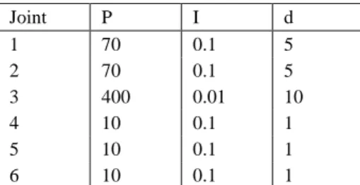
Table 8
PSM PID Values used during trajectory tracking
Joint P I d
1 70 0.1 5
2 70 0.1 5
3 400 0.01 10
4 10 0.1 1
5 10 0.1 1
6 10 0.1 1
Table 8 shows the tuned PID values for the mass and inertias given in Solidworks.
The results of this test are plotted in Figure 10, where left are the commanded (blue) and resulting (orange) joint trajectories, and right are tracking errors. This shows that all joints were tracking with good stability and minimal delay.
Table 9
Real time coefficient of different Gazebo configurations of the dVRK
Simulation Real time coefficient
PSM 1
ECM 1
2 PSM + ECM 0.98
3 PSMs 0.99
SUJ + 3 PSM + ECM 0.51
SUJ + 3 PSM + ECM + Camera
0.47
Figure 10
Joint trajectory tracking of the PSM in Gazebo Simulation. Left, commanded blue joint trajectory has similar values to orange actual joint trajectory.
During this test, the real-time coefficient is 1. This coefficient is automatically calculated and indicates the ratio between real-time and simulation time, as Gazebo can slow down simulation time as the computation cost of each iteration is increased. A test to determine the simulation load of different configurations is also conducted by measuring the real-time coefficient. The coefficient was not significantly affected by the commanded trajectory tracking but, rather, by the number of models in the simulation. Table 9 shows the results for each configuration test. The full model which included the camera plugin had a real- time coefficient of 0.47.
Conclusions
This work provides an approach for developing closed-loop kinematic chain models, using existing serial chain models applied to the da Vinci Surgical System. An optical motion capture system was used to calibrate the link lengths of the four-bar linkage mechanism of the PSM/ECM. This procedure can also be applied to other robots with a similar parallel axis closed-loop kinematics. Due to variations in the physical configuration among da Vinci systems, this calibration method could be used to update models for another specific da Vinci System.
Furthermore, the models were used and verified for ROS based simulations in RViz and Gazebo. Verification of the remote center of motion location of the PSM and ECM manipulators showed acceptable errors as compared to the hardware RCM. Additionally, this work verifies the stability and performance of the dynamic simulation using a joint trajectory tracking test of the PSM where
every joint succeeded in stable tracking of a sinusoidal wave. Finally, a test was conducted to measure the simulation load with various model configurations.
CAD Models and simulations are available at https://github.com/WPI- AIM/dvrk_env
Acknowledgement
This work has been supported by National Science Initiative NSF grant: IIS- 1637759
References
[1] Satava, R. M., (2003) Robotic surgery: from past to future--A personal journey. Surgical Clinics of North America, 83(6), pp. 1491-1500
[2] Bodner, J., Wykypiel, H., Wetscher, G. and Schmid, T., (2004) First experiences with the da Vinci operating robot in thoracic surgery. European Journal of Cardio-thoracic surgery, 25(5), pp. 844-851
[3] Okamura, A. M., (2009) Haptic feedback in robot-assisted minimally invasive surgery. Current opinion in urology, 19(1), p. 102
[4] Pandya, A., Reisner, L. A., King, B., Lucas, N., Composto, A., Klein, M.
and Ellis, R. D., (2014) A review of camera viewpoint automation in robotic and laparoscopic surgery. Robotics, 3(3), pp. 310-329
[5] Park, S., Howe, R. D. and Torchiana, D. F., (2001) October. Virtual fixtures for robotic cardiac surgery. In International Conference on Medical Image Computing and Computer-Assisted Intervention (pp. 1419-1420) Springer, Berlin, Heidelberg
[6] Sen, S., Garg, A., Gealy, D. V., McKinley, S., Jen, Y. and Goldberg, K., (2016 May) Automating multi-throw multilateral surgical suturing with a mechanical needle guide and sequential convex optimization. In Robotics and Automation (ICRA), 2016 IEEE International Conference on (pp.
4178-4185) IEEE
[7] Kazanzides, P., Chen, Z., Deguet, A., Fischer, G. S., Taylor, R. H., &
DiMaio, S. P. (2014 May) An open-source research kit for the da Vinci Surgical System. In Robotics and Automation (ICRA), 2014 ˝ IEEE International Conference on (pp. 6434-6439) IEEE
[8] Chen, Z., Deguet, A., Taylor, R. H., & Kazanzides, P. (2017 April) Software Architecture of the da Vinci Research Kit. In Robotic Computing (IRC), IEEE International Conference on (pp. 180-187) IEEE
[9] Khatib, O., (1987) A unified approach for motion and force control of robot manipulators: The operational space formulation. IEEE Journal on Robotics and Automation, 3(1), pp. 43-53
[10] Ulrich, N. and Kumar, V., (1991 April) Passive mechanical gravity compensation for robot manipulators. In Robotics and Automation, 1991 Proceedings, 1991 IEEE International Conference on (pp. 1536-1541) IEEE [11] Fontanelli, G. A., Selvaggio, M., Ferro, M., Ficuciello, F., Vendiuelli, M.
and Siciliano, B., (2018 August) A v-rep simulator for the da Vinci research kit robotic platform. In 2018 7th IEEE International Conference on Biomedical Robotics and Biomechatronics (Biorob) (pp. 1056-1061) IEEE [12] Perrenot, C., Perez, M., Tran, N., Jehl, J. P., Felblinger, J., Bresler, L. and
Hubert, J., (2012) The virtual reality simulator dV-Trainer® is a valid assessment tool for robotic surgical skills. Surgical endoscopy, 26(9), pp.
2587-2593
[13] Robotic Surgery Simulator. Available online:
http://www.simulatedsurgicals.com/ross.html (accessed on 5 November 2018)
[14] Moglia, A., Ferrari, V., Morelli, L., Ferrari, M., Mosca, F. and Cuschieri, A., (2016) A systematic review of virtual reality simulators for robot- assisted surgery. European urology, 69(6), pp. 1065-1080
[15] Rosen, J., MacFarlane, M., Richards, C., Hannaford, B. and Sinanan, M., (1999) Surgeon-tool force/torque signatures-evaluation of surgical skills in minimally invasive surgery. Studies in health technology and informatics, pp. 290-296
[16] Haidegger, T., Benyó, B., Kovács, L. and Benyó, Z., (2009) August. Force sensing and force control for surgical robots. In 7th IFAC Symposium on Modeling and Control in Biomedical Systems (Vol. 7, No. 1, pp. 413-418) [17] Quigley, M., Conley, K., Gerkey, B., Faust, J., Foote, T., Leibs, J., & Ng,
A. Y. (2009 May). ROS: an open-source Robot Operating System. In ICRA workshop on open source software (Vol. 3, No. 3.2, p. 5)
[18] Kam, H. R., Lee, S. H., Park, T. and Kim, C. H., (2015) Rviz: a toolkit for real domain data visualization. Telecommunication Systems, 60(2), pp.337- 345
[19] Koenig, N. P. and Howard, A., (2004) September. Design and use paradigms for Gazebo, an open-source multi-robot simulator. In IROS (Vol. 4, pp. 2149-2154)
[20] Bailey, M., Gebis, K. and Zefran, M., (2016) Simulation of closed kinematic chains in realistic environments using gazebo. In Robot Operating System (ROS) (pp. 567-593) Springer, Cham
[21] Gamage, S. S. H. U. and Lasenby, J., (2002) New least squares solutions for estimating the average centre of rotation and the axis of rotation.
Journal of biomechanics, 35(1), pp. 87-93
[22] Nycz, C. J., Meier, T. B., Carvalho, P., Meier, G. and Fischer, G. S., (2018) Design Criteria for Hand Exoskeletons: Measurement of Forces Needed to Assist Finger Extension in Traumatic Brain Injury Patients. IEEE Robotics and Automation Letters, 3(4), pp. 3285-3292
[23] SolidWorks to URDF Exporter. Available online:
http://wiki.ros.org/sw_urdf_exporter (accessed on 5 November 2018) [24] Open Source Robotics Foundation. SDF, Describe your world. Available
online: http://sdformat.org/ (accessed on 5 November 2018)
[25] Yaniv, Z., (2015) March. Which pivot calibration?. In Medical Imaging 2015: Image-Guided Procedures, Robotic Interventions, and Modeling (Vol. 9415, p. 941527) International Society for Optics and Photonics [26] Coumans, E., (2010) Bullet physics engine. Open Source Software:
http://bulletphysics.org, 1, p. 3
![Table 7 summarizes the RCM verification results for both PSM and ECM. The absolute position error of the simulation compared to the hardware is 3.46 [mm]](https://thumb-eu.123doks.com/thumbv2/9dokorg/1238423.95633/15.748.119.630.728.843/summarizes-verification-results-absolute-position-simulation-compared-hardware.webp)