Suboptimal and conflict-free control of a fleet of AGVs to serve online requests
M´ arton Dr´ otos
∗, P´ eter Gy¨ orgyi
†, Mark´ o Horv´ ath
‡, Tam´ as Kis
§September 24, 2020
Abstract
In this paper we propose a centralized control method for routing and scheduling a fleet of autonomously guided vehicles that serves online transportation requests. Our method maintains a central schedule, which is revised each time a vehicle finishes its current transportation task or a new transportation request arrives. The main benefit of the central schedule is that it ensures provably conflict-free control of a large fleet of vehicles on almost any layout, and permits optimization taking all the ve- hicle routes and schedules into account at the same time. We pay special attention to parking vehicles which may block the way of the moving ve- hicles, and our method inserts pull-off routes for them. The schedules are improved by various strategies, such as reducing the delays by swapping the order of the vehicles crossing the same lane, or elimination of loops in the vehicle routes created by pull-offs. We demonstrate the capabilities of our method by a series of computational tests, in which we also compare our mechanism to a recent conflict-free centralized method which is also designed for handling online requests.
1 Introduction
Autonomously guided vehicles (AGVs) are widely used in modern manufactur- ing systems, and they are the source of several challenging research problems as well. In this paper, we deal with the high level control of a fleet of AGVs, and our goal is to ensure conflict-free operation while serving transportation re- quests arriving over time. A somewhat neglected, but very important measure of the performance of a control system is the total delay or tardiness of serv- ing the requests. However, to our best knowledge, this performance measure is dealt with in the scientific literature mostly in off-line problems, where the transportation requests are known a-priori, see e.g., Murakami (2020).
∗drotos.marton@sztaki.hu
†gyorgyi.peter@sztaki.hu
‡horvath.marko@sztaki.hu
§kis.tamas@sztaki.hu
Specifically, we focus on problems of the following kind. There is a fleet of AGVs to serve pickup-and-delivery requests that arrive online. Fulfillment of a request consists of one or two stages: (i) an AGV has to be sent to the pickup station of the request, unless one is already waiting there, and after the item is loaded, (ii) the AGV transports it to the delivery station, where the item is unloaded from the AGV. It is assumed throughout the paper that the AGVs can move only on some pre-selected corridors, which is quite common in densely built-in factories and warehouses. These corridors help to avoid accidents with people, but they do not exclude the possibility of different conflict situations among the vehicles.
While avoiding physical collisions is not too difficult today (by appropriate sensors and hardware that stops a vehicle if it is too close to an obstacle or to another vehicle), guaranteeing that each request gets served is much harder.
There are two main types of conflicts that may prohibit the serving of requests:
deadlocks (when some vehicles cannot move), and live locks (when some vehi- cles get into an infinite loop of movements). The resolution of these conflict situations, if they occur, usually requires expensive human intervention. Auto- matic avoidance of conflicts can be achieved by a sophisticated control system, where we distinguish two main types: centralized anddecentralized ones. In a centralized system, a central unit communicates with the vehicles, and carries out various complex tasks, such as path planning, or motion coordination of the vehicles. In case of large layouts, path planning and motion coordination are usually performed separately to reduce the complexity (see e.g., Draganjac et al. (2016)), which is typically the main drawback of centralized systems.
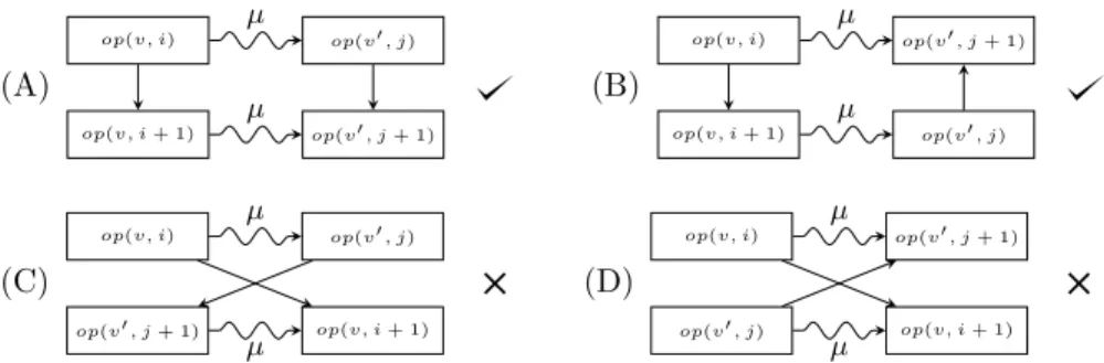
The main advantage of the decentralized control systems are the elimination of heavy computational tasks, and responsiveness to ad-hock traffic situations, and to changes in the environment. In such a system, the vehicles plan their own routes without any central unit. The main drawback of a decentralized system is the higher chance of emerging conflict situations. Many papers (see Section 2) deal with detecting and solving newer and newer types of conflicts, see Figure 1 for some examples. The first three types are quite well-known, and there are several (even decentralized) approaches to deal with them. In the last one, there is a full room (i.e., there is no place for more AGVs), and another AGV needs to get into this room through the only narrow corridor. Solving such a conflict is usually problematic for a decentralized system, while it is easier to avoid, or solve for a centralized one. Decentralized systems guarantee only a local solution, i.e., the way of resolving one conflict may lead to a new conflict situation, and resolving that to another conflict situation, etc. Another drawback of the decentralized systems is the lack of global optimization of costs related to total travel distances, and delays in serving the requests. To sum up, according to our knowledge, currently there is no decentralized method that guarantees a global conflict-free control of the vehicles, specifically, when the number of the vehicles is large, or the layout is complex (e.g., there is only a narrow corridor connecting two rooms, or if the layout has a tree-like structure).
We propose a centralized approach guaranteeing conflict-free operation of a large fleet of vehicles. The main advantages are as follows:
(A) (B) (C) (D)
Figure 1: Examples for conflicts. Boxes are vehicles, the gray vehicles are parking. Facing conflict (A), intersection conflict (B), node occupancy conflict (C), and full small room conflict (D).
• The created plans are conflict-free, i.e., with appropriate control, no dead- lock or live lock may occur. The conflict-freeness of plans is guaranteed by their structure.
• Our method does not require the identification or classification of possible conflict situations. Thus, it can handle all of the examples in Figure 1 at once, and many others.
• We can handle idle blocking vehicles, and unlike most other papers, vehi- cles with common target locations. While resolving these issues, no further conflicts are created.
• Our approach supports the optimization of plans, and we describe a method based on local search.
• We have only very mild assumptions on the layout, and we permit both one-way and bidirectional corridors. Thus, our method can handle most layout types that occur in practice.
• Our approach requires only low computational time, thus it avoids the main drawback of centralized methods. It scales up well with the number of AGVs, and the size of the network.
• It outperforms the method of Ma lopolski (2018) with respect to average tardiness of the requests, and to a new performance measure, introduced in this paper.
The new performance measure describes the operation of the system dur- ing the whole time horizon, and it is able to compare different problems, and methods in the future in a more proper way than the standard measures such as average tardiness. Our method is compared to the method of Ma lopolski (2018), which, according to our knowledge, is the only complete method so far. All of our benchmark data, and result files are freely available from the authors. We note that this paper does not apply a sophisticated method for task allocation (for such a method we refer to e.g., Gy¨orgyi and Kis (2019)), since our main
goal is to determine a conflict-free schedule and execution where the average tardiness of the requests is minimal.
The paper Ma lopolski (2018) claims that, the static methods (that find routes in advance and cannot react dynamically to traffic conditions) devel- oped hitherto, are suitable for small transportation systems, but admits the great potential in this area. Our approach is a new attempt in this direction.
In Section 2 we briefly overview the related literature. In Section 3, we give a detailed problem statement. Then, in Section 4, we describe our method in detail, and prove that under proper execution, it is conflict-free. In Section 5, we present our benchmark data, and computational results. We conclude the paper in Section 6.
2 Literature review
There is a long, detailed review in Ma lopolski (2018) on the different approaches, classifying the papers according to various attributes. Based on this review, we provide brief explanation of the theoretical foundations and classifications of the topic. We emphasize the most relevant articles from the literature, and also concentrate on recent results.
The simplest classification is based on the layout of the considered prob- lem. Several papers deal with conflict-free routing on specific layouts, like a grid (mesh), or a loop. Grids describe networks at warehouses or container terminals, where the layout contains regular blocks. For such a layout, the de- centralized methods of Rong (2017), Liu et al. (2017), and Zhang et al. (2018) detect more and more types of conflicts (like intersection conflict, catching-up conflict, node occupancy conflict, etc.), and provide solution algorithms to avoid them, but they do not guarantee the avoidance of newer conflicts. Central- ized methods are also considered for such layouts, see e.g., Banaszak and Krogh (1990), Ghasemzadeh et al. (2009), Bocewicz et al. (2014), Cardarelli et al.
(2017).
If the layout does not have any specific attributes (i.e., it isconventional), then there is no chance to list the possible types of conflicts and deal with them one-by-one. Another important question is whether the system allows only unidirectional paths on narrow corridors or not. Allowing bidirectional paths increases the throughput while using a smaller number of vehicles, however, it also increases the number, and the types of possible conflicts Egbelu and Tanchoco (1986). For further results, see e.g., Daniels (1988), Taghaboni-Dutta and Tanchoco (1995), Draganjac et al. (2016), or Ma lopolski (2018).
Another classification scheme is based on the type of solving algorithms. We distinguish static, time-window based, and dynamic methods. Static solution algorithms mainly require very strong assumptions, like the branch-and-bound procedure of Daniels (1988), where the network model permits that several vehicles wait at the nodes. Without strong assumptions (except that the final destination of all vehicles must be distinct), some theoretical methods could be applied, such as those for solving thepebble motion problem on a graph, which
generalizes the classic 15-puzzle. In this problem, there is a graph, and there are pebbles on some nodes of the graph (at most one pebble on each node). It is feasible to move a pebble to a neighboring node if it is empty, and the objective is to reach a given final configuration of the pebbles by a series of feasible moves.
It can be decided in polynomial time whether it is possible or not Kornhauser et al. (1984). This problem can be adapted to solve any control problems without conflicts, namely, the vehicles are the pebbles that move among the nodes of a graph which represents the layout. However, this result is theoretical, and it does not consider e.g., the due dates of the transportation requests, and it does not permit that two vehicles have a common destination. The method of Ma lopolski (2018) is also theoretical, but it is designed for conflict-free control of AGV systems. It assumes that each vehicle has a dedicated depot node, where it cannot block the route of any other vehicle, see the Appendix for more details.
There are other centralized conflict-free methods with slightly more practical relevance like Miyamoto and Inoue (2016), Murakami (2020), and Zhong et al.
(2020), which formulate the problem as a mixed-integer linear programming (MILP) problem, and then solve it by an exact method or by a heuristic. These methods require large computation times, thus the presented instances of the first two papers contain at most three AGVs, while the latter paper works on a layout with a couple of edges and nodes. Consequently, they cannot be applied in an online setting where the requests arrive online. Another drawback is that they assume the same distance among the neighboring nodes, hence, the size of the underlying graph may be very large in practical applications. The method of Ryan (2008) partitions the map into subgraphs of known structure with entry and exit restrictions to reduce the computational times, thus it can deal with instances with 10 or even 20 vehicles. Nevertheless, this method sometimes fails, thus it needs another mechanism (with more computational time) as a backup.
Time-window based solution approaches. In the series of articles M¨ohring et al. (2005); Gawrilow et al. (2008); Stenzel (2008); Gawrilow et al. (2012), an application for a container terminal is described. These papers use a so-called time-expanded graph in which arcs are labeled with time intervals dedicated to vehicles. When seeking a new route for a vehicle, only the free time windows of the arcs can be used. However, this approach does not deal with the problem of blocking parking vehicles (e.g., if there is a parking vehicle in the final node of a route, then there is no feasible solution unless the blocking vehicle gets a pull-off route), which is a common problem in applications Bruno et al. (2000);
Kim and Park (2009). Unfortunately, the computational results of Gawrilow et al. (2012) are confidential, so we get no details about the performance of the method.
Dynamic methods. These methods can modify the route of a vehicle based on real time traffic information. For more details, see e.g., Taghaboni-Dutta and Tanchoco (1995), Bartlett et al. (2014), or articles where the dynamic approach is combined with time-windows (e.g., Gawrilow et al. (2008), Smolic-Rocak et al.
(2009)).
The third possible classification is based on the control mechanism, which
can be centralized or decentralized, see Section 1. There are methods like Digani (2016) with a partly centralized, partly decentralized approach: similar to Ryan (2008), it partitions the layout into disjoint zones, and then applies a central database to store traffic data which facilities the high level planning of the routes of the vehicles between the zones. Within the zones, the vehicles plan their own paths while communicating with each other. This method can bound the number of the vehicles within each zone, thus decreasing the chance of conflicts between them.
There are several ways to model the layout or the movements of the vehicles.
Most of the cited articles use a graph representation of the layout, i.e., the intersections are represented by nodes and the corridors by edges. We would like to note that several articles use Petri nets for modeling some aspects of the problem. For instance, Petri nets can describe the usually fixed routes of the vehicles, and they help to identify conflicts, or to decide the order of vehicle movements, e.g., in Zeng et al. (1991) colored Petri nets are used for detecting conflicts. They can also be applied for analyzing control mechanisms, e.g., Castillo et al. (2001). However, for route planning usually additional techniques are needed, which work directly on the network representation of the problem.
We are not aware of results that use Petri nets for resolving conflicts due to idle vehicles, or vehicles with a common destination. E.g., Wu and Zhou (2001) excludes idle vehicles, and Nishi and Maeno (2010) deals with fixed routes and requires that each vehicle has a unique start and destination points.
We will apply some ideas from scheduling theory, see e.g., Blazewicz et al.
(2019). In particular, in a no-wait job-shop scheduling problem each job is a chain of operations, where each operation requires one machine, and when some operation, except the last one, of a job completes, the next operation must start immediately, see e.g., Samarghandi (2019) and the references in it. However, in the classical no-wait job-shop model, the processing times of the jobs are fixed, and each resource can process only one job at a time. In contrast, as we will see in Section 4, in our schedules the operations have no fixed processing times, those requiring the same resource may overlap in time, and they have to meet additional conditions which are unknown in no-wait job-shop scheduling.
3 Problem statement
In this section we describe the most important ingredients and modeling assump- tions about the AGV system for which in Section 4 we propose a conflict-free and efficient control mechanism.
The physical environment in which the AGVs move consists of one or more production halls or yards, divided into corridors by the placement of machining centers and storage units. So it is a network of narrow and wide streets which meet at intersections. A narrow street has a single lane, where the vehicles cannot overtake or bypass each other, while a wide street has two or more parallel lanes, but the vehicles cannot switch lanes. The traffic in a single lane can be one-way (the direction of traffic is fixed and does not change), or
Figure 2: Example for a graph representation of a simple factory layout. The red nodes represent stations, and the green ones the parking places. The arrows indicate the directed edges.
bidirectional (traffic may pass in both directions, but not at the same time).
This permits e.g., that in parallel lanes traffic may pass simultaneously in both directions. There are some special locations, so-calledstations, where the AGVs stop for pickup and drop-off, andparking places, where idle vehicles may wait for the next request. Stations may be located near machining centers and storage units for loading/unloading parts or pallets, while parking places are typically at the end of blind paths, but any other location can be designated as a parking place. Stations may serve as parking places as well, and we emphasize that parking places are not dedicated to vehicles in our approach. There are some mild rules for selecting the parking places, see Assumptions 1 and 2 below.
After these preliminaries, we can formally describe our problem. The most important problem data are the set of vehicles V, the set of (online) requests R, and a mixed graph G = (N, A) which describes the layout. The nodes in N represent the stations, the intersections of the lanes, and the parking places.
The undirected arcs in A correspond to lanes with bidirectional traffic, while directed arcs model one-way lanes, see Figure 2. However, parallel edges (two edges connecting the same pair of nodes) are not allowed. The intersection of wide streets, where several lanes meet, are modeled by several nodes and edges among them. Finding a good graph representation of a factory or warehouse is out of scope, this paper assumes that the graph is fixed in advance.
We have only two simple assumptions onG:
Assumption 1. BothG, and the graph obtained fromGby removing the nodes corresponding to the parking places are strongly connected1.
Assumption 2. The number of the parking places is at least one more than the number of the vehicles.
1A mixed graph isstrongly connectedif there is a path from any nodeuto any other node vsuch that each arc of the path is either undirected, or its direction is aligned with that of the path.
In most practical applications, both assumptions hold, or easy to achieve. A notable exception is whenGis just a cycle, without any pendant nodes.
Each vehicle inV has an initial location, and they have common maximum speed (on straight routes and in bends), maximum acceleration, and physical dimensions. The minimum safety distance between any two vehicles is also given. Each vehicle can transport only one item at a time. The vehicles obey some physical constraints during their movements:
P1) As the vehicles move, they respect the maximum speed (i.e., they cannot go faster), the maximum acceleration, and the safety distance.
P2) There can be at most one vehicle in any intersection or in any station simultaneously.
P3) The vehicles can neither overtake one another, nor go in the opposite di- rection simultaneously in the same lane.
P4) Changing direction in lanes is not allowed.
We define a capacity for each g ∈ N ∪A. For the nodes g ∈ N, c(g) := 1, whereas for an edgeg ∈A, c(g) is the maximum number of vehicles that can reside in the corresponding lane, when both end nodes are occupied by a vehicle, while respecting the safety distance between the vehicles. An edgegisshort if c(g) = 0, otherwise it islong.
The vehicles have to serve a sequence of requests R, which are not known a-priori, but arrive one-by-one over the time horizon, e.g., a working day. Each request r ∈ R has an arrival or announcement time ar, and prescribes the transportation of a single item (part or pallet) from one station to another.
A request r is determined by its pickup and delivery stations, pickup time er
(loading cannot start before er), duration of loading and unloading, and due date dr. We emphasize that the problem is online, i.e., each request r ∈ R becomes known only after its announcement time ar. Typically, ar < er < dr
hold.
A vehicle serves a requestrif it loads the corresponding item at the pickup station of the request (but not earlier than er), then carries it to the delivery station, and finally unloads the item. A request isfinishedif the item is unloaded at the delivery station. We assume that once an item is loaded, it cannot be unloaded until the AGV carrying it stops at the delivery station.
The solution of the problem is a schedule of the vehicles on the nodes and edges of G. The schedule consists of operations, where each operation repre- sents either going through a lane (edge), or crossing an intersection (node), loading/unloading at a station (node), or waiting at a location (node). Each vehicle has a routing (sequence of operations), and for each node or edge, those operations that require it are totally ordered. A schedule is not static, it evolves over time, and even scheduled vehicle movements can be replaced by another ones. A more formal definition of schedules will be given in Section 4.1. A schedule of the vehicles isfeasible, if
• each request is served by a vehicle, while the load operation of the request is started not sooner than the pickup time of the request, and
• it can be physically realized while respecting P1-P4.
If a request r is finished at time point t then the tardiness of r is Tr :=
max{0, t−dr}. If Tr= 0 then ris served on time, otherwise, it istardy. The objective is to find a feasible schedule (over time) of the vehicles where the average tardinessP
r∈RTr/|R|is minimized.
4 Description of our method
In this section we give a detailed description of our techniques. Firstly, we give a high level overview in Section 4.1, then we describe schedules in Section 4.2, which constitute the main data structure manipulated by the various algorithms.
In Section 4.3 we explain how the schedules are updated with new requests, or when some AGV is delayed, and in Section 4.4 we propose a local search procedure for improving the schedules. Finally, in Section 4.5 we briefly sketch a schedule execution mechanism to be implemented in the AGVs.
4.1 Overview
Our method maintains a feasible schedule (defined in Section 4.2) and if new requests arrive, and there is at least one free vehicle (or a vehicle become avail- able and there is at least one unprocessed request), the schedule is updated so that the vehicles serve the assigned requests. We mention right at this point that even if there is a free vehicle when a new request arrives, maybe the system waits until another vehicle becomes free (after serving a request), if that vehicle can do the job with a smaller delay.
Our method performs the following steps each time a request is finished, or a new request arrives:
1. Assignment of AGVs to transportation requests. There is at most one request assigned to each AGV at a time. If a new request is announced or an AGV becomes available (it has finished its previous request) we invoke a simple assignment algorithm:
(i) Put the unassigned requests in increasing pickup time (er) order;
(ii) If there is no unassigned request or each AGV has a request, then STOP;
(iii) Letrbe the first unassigned request;
(iv) For each AGV without a request, determine the time point when it can arrive to the pickup location ofr. Assignrto the AGV with the smallest value. Go to Step 1ii).
2. Planning and replanning of the AGVs. Once a request is assigned to a vehicle, two routes in the network has to be selected: (1) from the vehicle’s last location in the schedule to the pickup station of the request, and (2) from the pickup station to the delivery station. Then, both routes have to be scheduled. The consistency of the schedule will ensure that no deadlock may occur. A detailed description of (re)planning can be found in Section 4.3.
3. Improve the schedule. After each rescheduling we invoke a procedure for improving the schedule, see Section 4.4 for details.
In the above procedure, the control of AGVs is missing, as it runs indepen- dently of the above planning process, and separately in each AGV, for details see Section 4.5.
4.2 Schedules
A resource is a node or a long edge of the layout graph G = (N, A) (short edges have no corresponding resources). Anoperation of a vehiclev represents either going through a long edge, or a node, or the loading / unloading of a request at a node. We say that v occupies a resource, if its center is located in the corresponding physical space (intersection/station for nodes and lane for edges). Aschedule S specifies for each vehiclev∈ V a routing (sequence of operations)L(v) = (op(v,1), . . . , op(v, last(v)) along with the required resources µ(v, i) ∈ N ∪A, 1 ≤ i ≤ last(v), and also for each resource g ∈ N ∪A, a sequenceL(g) = (op(v1, i1), . . . , op(vlast(g), ilast(g))) specifying a total order of those operations that require g, i.e., µ(vk, ik) = g for 1 ≤ k ≤ last(g). In addition, each operationop(v, i) has a time interval [ts(v, i), te(v, i)] specifying whenvoccupies the resourceµ(v, i). Letpmin(v, i) be the minimum time needed for vehiclevto performop(v, i). Clearly, ts(v, i) +pmin(v, i)≤te(v, i).
A schedule isfeasible if it admits a feasible realization, i.e., the vehicles can move precisely as the schedule prescribes it while respecting the timing of the operations and the physical constraints P1-P4 of Section 3. Our next goal is to characterize feasible schedules. LetOP =∪v∈VL(v) be the set of all operations, and we define the partial order≺µ⊂OP ×OP such thatop(v, i)≺µ op(v0, j) if and only if µ(v, i) = µ(v0, j) and op(v, i) precedes op(v0, j) in the sequence L(µ(v, i)). Recall that each resource g has a capaciyc(g). The following rules must be observed:
S1) For each vehicle v, µ(v,1) and µ(v, last(v)) must be node resources (the vehicles’ routes start and end on nodes of the layout graph), and for any pair of distinct vehicles v and v0, µ(v,1) 6= µ(v0,1), and µ(v, last(v)) 6=
µ(v0, last(v0)).
S2) For each vehicle v, and 1 ≤i < last(v), µ(v, i) andµ(v, i+ 1) cannot be both edge resources. Ifµ(v, i) is a node andµ(v, i+ 1) is an edge, then (a) µ(v, i) must be one of the end nodes of µ(v, i+ 1), or vice versa, and (b)
µ(v, i+ 2)6=µ(v, i). Ifµ(v, i) andµ(v, i+ 1) are both node resources, then these two nodes must be connected by a short edge of the layout graph.
S3) For any pair of consecutive operationsop(v, i),op(v, i+ 1) of a vehiclevthe following hold:
• If there existop(v0, j), op(v0, j+1)∈OP such thatop(v, i)≺µop(v0, j) andµ(v, i+ 1) =µ(v0, j+ 1), then op(v, i+ 1)≺µop(v0, j+ 1).
• If there existop(v0, j), op(v0, j+1)∈OPsuch thatop(v, i)≺µop(v0, j+
1) andµ(v, i+ 1) =µ(v0, j), thenop(v, i+ 1)≺µop(v0, j).
S4) For each operationop(v, i),ts(v, i) +pmin(v, i)≤te(v, i) and if i < last(v),
thents(v, i+1) =te(v, i). For each sequenceL(g) = (op(v1, i1), . . . , op(vlast(g), ilast(g))), (g ∈ N ∪A), ts(vk, ik) < ts(vk+1, ik+1), te(vk, ik) < te(vk+1, ik+1) for
1 ≤ k < last(g), and te(vk, ik) ≤ ts(vk+c(g), ik+c(g)) for each 1 ≤ k ≤ last(g)−c(g).
The condition S1 is a technical assumption to facilitate the localization of ve- hicles, it says that each vehicle has a distinct start node and a distinct end node. Condition S2 expresses the structure of vehicle routings, and guarantees P4. This rule describes that the vehicles can move only between neighboring nodes and edges and cannot turn around on any of the edges. Note also that if two nodes are connected by a short edge, then the short edge has no cor- responding operation in the routings of the vehicles. Condition S3 is derived from P3 and P1, see Figure 3 for an illustration. The first part of this con- dition excludes the possibility of overtaking (i.e., if a vehicle starts to use a resource earlier than another vehicle, then it is impossible that the second ve- hicle ends the usage of this resource earlier than the first vehicle), while the second guarantees that if a vehicle moves e.g., from a node to an edge, then no other vehicle can move in the opposite direction simultaneously. Finally, the timing relations in S4 are natural and follow from P3, except possibly the last relationte(vk, ik)≤ts(vk+c(g), ik+c(g)). On node resources, it ensures that each intersection/station is occupied by at most one vehicle at a time, cf. P2.
On edge resources, it allows at most c(g) vehicles to occupy the same edge g simultaneously, which may be a bit restrictive, but surely guarantees that the schedule can be realized in the physical environment.
To facilitate the computation ofts(v, i) andte(v, i), we define event graphs.
Anevent graph D˜ = ( ˜N ,A) is defined with respect to the routings˜ L(v),v∈ V, and operation ordersL(g), g ∈N ∪A, where ˜N contains a start event s(v, i) and an end evente(v, i) for each operationop(v, i). The set of arcs ˜Acomprises routing arcs for the vehicles, and ordering arcs for resources. The routing arcs are as follows: for each start event s(v, i), ˜Acontains the arcs (s(v, i), e(v, i)), and if i < last(v), then also (s(v, i), s(v, i+ 1)), and (s(v, i+ 1), e(v, i)), see Figure 4 for an illustration.
For each resourceg, the set ˜Acontains the arcs (s(vk, ik), s(vk+1, ik+1)) and (e(vk, ik), e(vk+1, ik+1)) for 1≤k < L(g), and the arcs (e(vk, ik), s(vk+c(g), ik+c(g)))
(A)
op(v, i) op(v0, j)
op(v, i+ 1) op(v0, j+ 1)
µ
µ (B)
op(v, i) op(v0, j+ 1)
op(v, i+ 1) op(v0, j)
µ
µ
(C)
op(v, i) op(v0, j)
op(v, i+ 1) op(v0, j+ 1)
µ
µ
(D)
op(v, i) op(v0, j+ 1)
op(v, i+ 1) op(v0, j)
µ
µ
Figure 3: Illustration of condition S3): (A) and (B) represent feasible subgraphs, while (C) and (D) violate the condition. The wavy arrows indicate ≺µ, while a straight arrow always points to the consecutive operation on a routing of a vehicle.
s(v, i) e(v, i)
s(v, i+ 1) e(v, i+ 1)
Figure 4: Vehicle edges for two consecutive operations of vehiclev.
for each 1≤k≤last(g)−c(g), cf. condition S4. See Figure 5 for an illustration.
Proposition 1. If an event graph has no directed cycles, then a timing of the events can be computed such that they satisfy S4.
The proof can be found in the Appendix.
We say that a schedule is proper if it satisfies conditions S1-S3, and the associated event graph has no directed cycles. In fact, by Proposition 1, proper schedules also satisfy condition S4.
4.3 Planning and replanning
In this section we describe how the current schedule is updated if a new request is assigned to an AGV, see Section 4.1. The current schedule describes a route for each vehicle to serve its current request, if any, but it does not contain the operations for finished requests.
The update of a schedule consists of two steps. First, we delete most of the operations (except the next few operations of each vehicle), and then we insert the new and the old routes into this schedule in some order, see below. Prelimi- nary computations have confirmed that it is a better strategy than augmenting the current schedule with new requests only.
s(v1, i1)
e(v1, i1)
s(v2, i2)
e(v2, i2)
s(v3, i3)
e(v3, i3)
s(v4, i4)
e(v4, i4) Figure 5: Ordering edges (first type: solid, second type: dashed) and some vehicle edges (dashdotted) for four consecutive usage of some edge resourceg.
Before we cut back the schedule, for each vehiclev we freeze the operations of the route L(v) from the beginning until v reaches the second node of the layout graph from its current position. Then, we delete most of the unfrozen operations with the following procedure:
Procedure Cut-back
Input: schedule with some frozen operations.
Output: new schedule graph
1. While there is a node resourceg, such that the last memberop(vlast(g), ilast(g)) ofL(g) is not the last operation ofL(vlast(g)), and the next operation of vlast(g)is neither finished, nor frozen, perform the following step:
2. Delete each operation inL(vlast(g)) afterop(vlast(g), ilast(g)).
Proposition 2. The schedule we get after procedure Cut-back, is feasible.
Proof. For eachv 6=v0 ∈ V, µ(v, last(v))6=µ(v0, last(v0)) holds after cut back, thus condition S1 holds. Deleting some operations from the end of the routes yields a schedule respecting S2-S3. Finally, apply Proposition 1.
Note that in the procedureCut-back, the freezing of operations is temporary only.
Now we show how to extend the shortened schedule so that the AGVs fulfill their assigned requests. In the following, ashortest path in the layout graphG from some nodens to another node ne is a shortest path among all the paths which do not contain a parking place as an internal node, i.e., onlynsornemay be parking places on the paths. Such a path always exists by Assumption 1.
We add the unscheduled requests one-by-one:
Algorithm Reschedule
Input: current schedule, set of vehicles with unscheduled requests Output: augmented schedule
1. Choose an unscheduled requestrwith an earliest due date.
2. Ifv is the AGV assigned tor, andµ(v, last(v)) equals the pickup location of r, or v has loaded the request, then we determine a shortest path in the layout graph from µ(v, last(v)) to the delivery station of r. Invoke procedureInsert Path to insert the corresponding sequence of operations into the schedule.
3. Otherwise, invokeInsert Path for a shortest path fromµ(v, last(v)) to the pickup station ofr, and for a shortest path from the pickup station to the delivery station ofr.
4. If there is at least one unscheduled request left, go to step 1.
The next procedure schedules the vehicles. The input is a vehicle v∗ and a pathP∗ from µ(v∗, last(v∗)) to a final destination node of the layout graph.
Scheduling a pair (v∗, P∗) consists of the generation of a sequence of operations corresponding to the nodes and edges ofP∗, and appending them to the current schedule, i.e., new operations are always appended after the last operation of each resource, and that of the route ofv∗. However, if some nodegon the path P∗ is blocked by a vehiclev0 6=v∗, i.e.,g=µ(v0, last(v0))∈P∗, then at firstv0 must get a pull-off route to a parking place of the layout graph. To complicate things, the way ofv0 may be blocked as well by another vehiclev00, so thatv00 should get a pull-off route first, etc. It may also happen that v∗ blocks the pull-off route of av6=v∗, thus v∗ itself must pull-off to some parking place to free the way forv. However, this can occur only once, see Proposition 4.
Procedure Insert Path
Input: current schedule, vehicle v∗, and a pathP∗ in the layout graph for v∗
Output: new schedule
1. LetV0 =∅ be the set of vehicles that require a pull-off route,L0 =∅ (it will be the set of the possible parking places), vehicle ¯v=v∗, path ¯P =P∗ (the ’actual’ vehicle and route).
2. Find blocking vehicles: extendV0with the set of vehiclesv0 6= ¯v such that µ(v0, last(v0))∈P¯.
3. Schedule (v∗, P∗) if v∗ is not blocked, i.e.,V0 =∅. Freeze every event of the schedule graph, except events of the pull-off routes. Invoke procedure Cut-back, and STOP.
4. If ¯vis not blocked, i.e., for anyv∈ V \{¯v},µ(v, last(v))∈/P¯, then schedule the pull-off route ¯P for the blocking vehicle ¯v. Delete ¯v fromV0.
5. Ifv∗has got a pull-off route in step 4, then let ˆP be a shortest path from µ(v∗, last(v∗)) to the last node ofP∗ and invoke procedure Insert Path for (v∗,Pˆ), and STOP.
6. Collect all parking places of the layout graph where a vehicle can be sent, i.e., letL0 be the set of parking places such that`0 is not an end node of P∗, and for anyv∈ V,µ(v, last(v))6=`0.
7. Select a vehicle to pull-off: for each v ∈ V0, let Pv be a shortest path among the paths fromµ(v, last(v)) to any parking place`∈ L0. Let ¯v, ¯P be such that ¯Pv¯is a shortest path among thePv,v∈ V0. Go to step 2.
(A)
n1 n2
n3
n4 n5 n6 n7
v2 v∗ v1 (B)
n1 n2
n3
n4 n5 n6 n7
v2
v∗ v1
(C)
n1 n2
n3
n4 n5 n6 n7
v2
v∗ v1
Figure 6: The initial state (A), the state after the pull-off of v∗ (B), and the final state (C).
The following example illustrates both the difficulties and the solution algo- rithm on a small layout graph.
Example 1. Consider the layout graph in Figure 6. Let n1, n2, n3, and n7
be parking places, and n7 a station as well. There are 3 vehicles, v1, v2 and v∗ located initially at the nodes n6, n4 and n5, respectively. All vehicles are idle, and v∗ gets a request so that it has to move to n7, thus it gets a path P∗ = (n5, n6, n7). Since v1 blocks v∗ on P∗, it must get a pull-off route first, i.e., V0 = {v1} after the first iteration. The closest parking place to n6 is n3 (apart from the n7 which is an end node of P∗), thus P¯ = (n6, n5, n4, n3) in step 7. Bothv∗andv2blocksv1, thus we add them toV0, and the new(¯v,P)¯ will be(v2,(n4, n3)). No vehicle blocks v2, thus we can schedule it along P¯. Then, we refreshv¯tov∗,P¯ to(n5, n4, n1)(becausen1 is the closest parking place not inP∗), and schedule it, because no vehicle blocks it. Since v∗ has got a pull-off route, the algorithm invokes itself for(v∗,(n1, n4, n5, n6, n7)).
After that, onlyv1blocksv∗ and it can be sent ton2, then the algorithm can schedule(v∗,(n1, n4, n5, n6, n7)).
First we prove the soundness of the Insert Path procedure.
Lemma 1. Suppose the current schedule is proper and let v ∈ V be a vehicle, andP a path in the layout graph from µ(v, last(v))to a node such that for any v0 ∈ V \{v},µ(v0, last(v0))∈/P. Then scheduling(v, P)yields a proper schedule.
Proof. Since for any v0 ∈ V \ {v}, µ(v0, last(v0)) ∈/ P, node µ(v, last(v)) in the updated schedule is different from anyµ(v0, last(v0)) forv0 ∈ V \ {v}, thus condition S1 holds. Since we insert each new operation after all the already scheduled operations on each resource, the other two conditions are also satisfied, and no directed cycle is created in the event graph.
Proposition 3. If the current schedule is proper, then the Insert Path procedure returns a proper schedule.
Proof. Observe that whenever the Insert Path procedure inserts a new path P for some vehiclev into the current schedule, then (v, P) satisfies the conditions of Lemma 1.
Now we turn to computational complexity.
Proposition 4. Procedure Insert Path is of polynomial time complexity on any input.
Proof. Letv∗be a vehicle,d∗any node of the layout graph, andP∗a path from µ(v∗, last(v∗)) tod∗. Suppose Insert Path is invoked on the input (v∗, P∗) and the current schedule.
First, we prove that the procedure cannot get stuck at step 7, i.e., ifV0 6=∅, then L0 6= ∅. If V0 6= ∅, then there is a blocking vehicle in d∗, or in a node of the layout graph which is not a parking place. It means that the number of those vehicles v with µ(v, last(v)) being a parking place node of the layout graph different from d∗ is at most |V| −1. Since the number of the parking places is greater than|V|(see the Assumption 2), there is at least one parking place different fromd∗which is not the last location of any vehicles, i.e.,L0 6=∅.
Now, we prove that the procedure invokes itself at most once, and each vehicle gets a pull-off route at most once. Let (˜v,P) be an arbitrary pair the˜ procedure tries to schedule. Since ˜P is a shortest path in the layout graph, it can visit a parking place only in its first or last node. The first node of ˜P is µ(˜v, last(˜v)), thus there is no vehicle v 6= ˜v such that the first node of ˜P is µ(v, last(v)). The last node of ˜P isd∗, or a parking place`0 of the layout graph such that µ(v0, last(v0)) 6= `0 for all v0 ∈ V. To sum up, if µ(v, last(v)) is a parking place of the layout graph different from d∗ for a vehiclev 6= ˜v, thenv cannot block ˜P.
If the procedure schedules a pull-off route for a vehiclev, then µ(v, last(v)) will be a parking place different fromd∗, thus the procedure schedules a pull-off route for each vehicle at most once, and after that it remains in the parking place except the vehiclev∗. If vehiclev∗ gets a pull-off route, then at step 5 the procedure invokes itself. During this second invocation, v∗ cannot block any vehicles, hence, it moves only once, tod∗.
At each iteration, the procedure either schedules a pull-of route for a vehicle, or adds some blocking vehicles to V0 (except the last iteration). Since the procedure deletes a vehiclev fromV0 only if it schedules a pull-off route forv, the procedure has at mostO(|V|) iterations. The running time of an iteration is polynomial in the size of the input, hence we have proved the proposition.
The results of this section boil down to the following statement.
Theorem 1. When applied to a proper schedule, the Reschedule algorithm de- livers a proper schedule in polynomial time.
4.4 Improvement of schedules
In this section we describe two methods for improving a schedule. The two methods are invoked repeatedly until they cannot improve the schedule.
Before describing the procedures in detail, recall the procedure Cut-back, which can be used to drop non-frozen events from a schedule. We also need some more definitions. Aloopin a route of a vehiclev is a subsequence of operations op(v, i), . . . , op(v, j) such that 1≤i < j≤last(v), andµ(v, i) =µ(v0, j) is the same node resource. Clearly, a loop may be eliminated if it contains neither the load nor the unload operation of a request served byvinternally (at some posi- tion strictly betweeniandj). By eliminating some loops, a schedule improves as the vehicles move less. Another option is to decrease the delays in a sched- ule. We say that the operationop(v, i) isdelayedifts(v, i) +pmin(v, i)< te(v, i).
Supposei < last(v), then ts(v, i+ 1) = te(v, i). Therefore, the delay may be caused by delaying the end ofop(v, i). Hence, to eliminate the delays, we may try to move the operation op(v, i+ 1) to some other position on the resource µ(v, i+ 1). The delays will be reduced repeatedly within a local search proce- dure. Firstly, we describe the complete method:
Procedure Improve Schedule Input: current schedule
Output: updated schedule
1. Freeze all the non pull-off operations, and cut-back the schedule.
2. Invoke the Loop Elimination procedure.
3. Decrease the delays of the operations by the Local-Search procedure.
4. If no changes occurred in the second or third steps, then STOP; otherwise proceed with step 1.
The main idea of the Loop Elimination procedure is that it identifies sub- routes of the vehicles starting and ending on the same node and not containing internally the pickup or the delivery operation of the request being served.
Procedure Loop Elimination Input: current schedule
Output: updated schedule
1. For each vehiclev perform the steps 2)-4).
2. Freeze the operations ofvuntil it reaches the second node from its current position, and letop(v, i) be this operation.
3. For eachk=itolast(v)−1 andk=j+1 tolast(v) perform the following:
4. Ifµ(v, j) =µ(v, k) is the same node resource, and the subsequenceL0 = (op(v, j), . . . , op(v, k)) does not contain a load or unload operation in- ternally, then remove L0\ {op(v, k)}, and test if the remaining schedule
S
op(v0, j−1) op(v, i+ 1)
op(v, i) op(v0, j)
S0
op(v0, j−1) op(v, i+ 1)
op(v, i) op(v0, j)
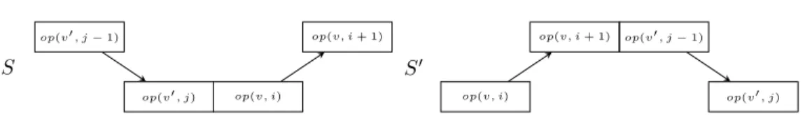
Figure 7: Example for Swap and Propagate, the operations in same line require the same resource. After the swapping order of op(v, i) and op(v0, j), we also need to swap the order ofop(v, i+ 1) andop(v0, j−1) (cf., Figure 3 (D)).
satisfies S1)-S3). If it does not, then reinsertL0\ {op(v, k)}, and proceed;
otherwise STOP.
Local search is a general technique to improve partial or complete solutions of an optimization problem, see e.g., Michiels et al. (2007). The main idea is that we define aa neighborhoodof the current solution, and then pick a neigh- bor with a better objective function value than the current one. In our case the solutions are feasible schedules. For a scheduleS, the set of critical operations are those op(v, i) such that i > 1, and op(v, i−1) is delayed, see above. For each critical operationop(v, i), we obtain a neighbor by swappingop(v, i) with its immediate predecessor on its resource. Clearly, swapping only these two operations may yield a schedule graph which does not satisfy the conditions S1)-S4). To remedy this, the swaps must be propagated by the following:
Procedure Swap and Propagate Input: scheduleS and operationop(v, i)
Output: scheduleS0in whichop(v, i) is swapped with it resource predecessor inS
1. Swapop(v, i) with its immediate resource predecessorop(v0, j).
2. LetH :={op(v, i−1), op(v, i+ 1)}, andK:={op(v0, j−1), op(v0, j+ 1)}
(omit those operations which do not exist).
3. For each pair (o, o0)∈H×K perform the following:
4. Ifoando0 require the same resource, andoprecedes (not necessarily im- mediately)o0 on the common resource, then move o0 right aftero. Invoke Procedure Swap and Propagate on the current schedule graph, ando0. The procedure tries to ensure the condition S3). Notice that each pair of operations is swapped only at most once, and thus the procedure terminates in polynomial time in the size ofS. See Figure 7 for illustration.
The following simple local search based method is used to decrease the total delays of the operations of a schedule. Briefly, it invokes repeatedly Swap and Propagate on the actual schedule and one of its critical operations, until a fea- sible schedule is obtained with a smaller sum of delays.
Procedure Local Search Input: scheduleS
Output: scheduleS∗ 1. LetS∗:=S.
2. Lettd∗ be the sum of the delays of the operations inS∗ with respect to its timing. Lettdbest=∞andSbest the empty schedule.
3. For each critical operationopofS∗ in turn, do the following:
4. Let S0 :=S∗. Invoke the Swap and Propagate procedure on S0 and op, and letSsw be the resulting schedule.
5. If Ssw represents a feasible schedule, and the total delay of it is smaller than tdbest, then replace Sbest with Ssw, and updatetdbest to the total delay of Sbest. Proceed with Step 4 if there is an unprocessed critical operation.
6. Iftdbest< td∗, replace S∗ withSbest, and proceed with Step 2, otherwise STOP.
Since the objective function must decrease in every major iteration of the Local Search procedure, it terminates in a finite number of steps.
4.5 Execution mechanism
It is mandatory that the vehicles faithfully follow the schedule to ensure deadlock- free execution. Therefore, before a vehiclev moves to a node from an edge, it has to check that other vehicles scheduled to pass beforev have already visited the node. If not,vhas to wait until the other vehicles pass. In practice, vehicles may ask the central controller if there is any vehicle to wait for before moving to a node.
As for edges, the vehicles can move to an edge as soon as they can while respecting the safety distance. Moreover, they have to wait far enough from the other end of the edge so that they do not block the way of other vehicles crossing the node before them (those vehicles arrive from and proceed to different edges).
When a vehicle leaves a node or an edge, then the corresponding operation is marked ”finished”.
5 Computational results
In this section we compare our method to that of Malopolski Ma lopolski (2018), which is also a centralized method that also guarantees collision free routing of the vehicles. Moreover, we analyze how the load of the system affects its performance in terms of meeting the due dates of the requests.
In our computational tests we have used different layouts and request gen- eration schemes. The instance files and the detailed results are freely available
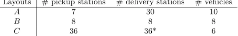
Table 1: The main features of the layouts. * indicates delivery stations are the same as pickup stations.
Layouts # pickup stations # delivery stations # vehicles
A 7 30 10
B 8 8 8
C 36 36* 6
from the authors. In Sections 5.1 and 5.2 we describe the layouts and request generation schemes, respectively. Then, we summarize our results in Section 5.3.
5.1 Layouts and vehicles
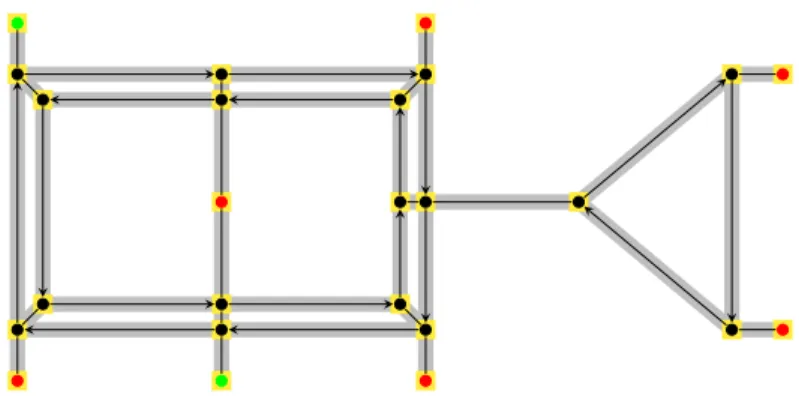
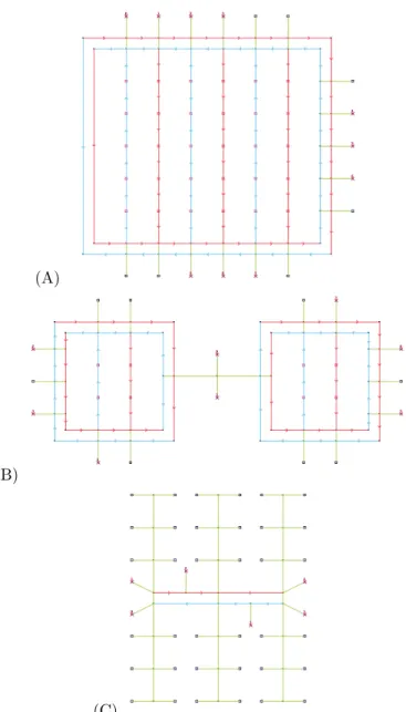
We have examined three different layout graphs that model some typical factory, and warehouse topologies, see Figure 8. LayoutA has a block structure with several parallel streets, inBthere are two rooms connected by a narrow corridor, while layout C has a tree-like structure. In layouts A and B, each station is either a pickup or a delivery station, while in C, there are universal stations where the requests can start as well as end.
The number of the vehicles for each layout is derived from its size. The characteristics of the layouts along with the number of vehicles are summarized in Table 1. Note that our method does not require so many parking places in the layout graphs, these are introduced only because the method of Ma lopolski (2018) requires that each vehicle has a separate depot node, and depot nodes must be different from stations.
5.2 Requests
A request contains the coordinates of the pickup and delivery stations, its an- nouncement timear, earliest pickup timeer, and due datedr. The pickup and the delivery station of a request is determined randomly (with a uniform distri- bution) among the pickup and the delivery stations. The pickup and delivery station of a request cannot coincide.
The pickup time of a request is a random number within the time horizon of 1000 time units. The announcement time of each requestris determined by ar = max{0, er−L}, where L is the estimated average service time, i.e., the expected value of the distance of the pickup station and the delivery station of a request, divided by the maximum speed of the vehicles. The due date of a request is determined by the following expression: dr=er+tL+tpd+tU L+ 60, wheretL is the loading time,tpd is the estimated time required for a vehicle to get from the pickup station to the delivery station (i.e., if the vehicle does not have to wait due to traffic), andtU L is the unloading time. In all of our tests, tL andtU L are set to 2 time units. The minimum time for serving the requests is extended by 60 time units to enlarge the time window of on-time delivery.
(A)
(B)
(C)
Figure 8: The three layouts, A, B and C. The initial location of a vehicle is denoted by an ’x’, a pickup node by a black square, and a delivery node by a red square (except in the third layout, where each pickup node serves also as a delivery node). Undirected edges are green, directed edges are red or blue.
For each layout, we have generated instances with two different number of requests, as determined by the following expression:
T imeHorizon· |V|
avgServT ime·α
,
whereT imeHorizon is the length of the time horizon (set to 1000),|V|is the number of the vehicles (different for each layout),avgServT ime is the average time required to serve a request (from loading to unloading, different for each layout), and factorα∈ {2,3}determines the overload of the system.
For each layout we have generated 100 instance files for both number of requests, giving a total of 600 problem instances.
5.3 Comparison to the method of Malopolski
We have implemented our method and the method of Malopolski in the Java programming language along with the improvement techniques. We have run both methods with, and without the improvements of Section 4.4. For our method, we have also considered the case, when we omit step 2 (Loop Elimi- nation) from Procedure Improve Schedule, and we just apply the local search procedure during the improvement. There is a short summary on the Malopol- ski method in the Appendix. The tests were run on a computer with i9-7960X CPU @ 2.80GHz, 16 cores 4x NVIDIA GeForce RTX 2080Ti, and Debian 9 Linux operating system. The entire simulation procedure was quite fast for any method and any instance file, it required approximately 5-15 seconds.
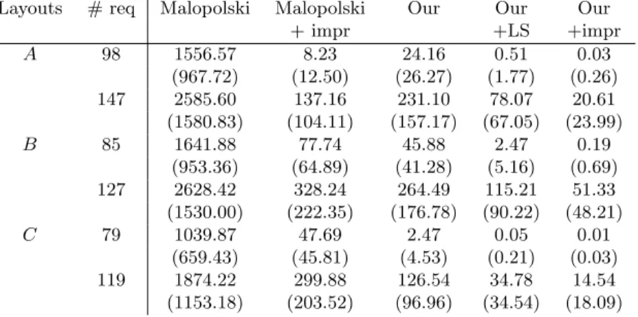
There are several important measures for an AGV system, firstly we focus on average tardiness, P
r∈RTr/|R|, of the requests. Table 2 summarizes the results, where each number is an average over 100 instances of the average tardiness of the requests. The standard deviations are in parenthesis. The columns determine the Layouts, the number of the requests (both for ofα= 3 and α= 2 for each layout), and the five methods, where ’+impr’ denotes the usage of Procedure Improve Schedule, while ’+LS’ denotes the usage of the local search heuristic only.
The results show that our method clearly outperforms that of Malopolski, which does not provide any comparable results without the improvement pro- cedures. The Local Search and the Improve Schedule Procedure help a lot in general, but in case of LayoutsB and C, our method has better results even without any improvement procedures than that of Malopolski with improve- ments. In all cases, the best results are obtained by our method when all improvement procedures are active, where the average tardiness is negligible whenα= 3 (when the number of the requests is relatively small). However, if α= 2, then the results show that the system is overloaded for all methods.
Tables 3 and 4 present the average empty and loaded travel distances, and times, respectively. The results show that our method not always use the short- est routes between the pickup and delivery stations unlike the method of Mal- opolski, which always does (see loaded travel distances). However, we do not
Table 2: Average tardiness: average values (and standard deviations) over 100 instances of the average tardiness of the requests.
Layouts # req Malopolski Malopolski Our Our Our
+ impr +LS +impr
A 98 1556.57 8.23 24.16 0.51 0.03
(967.72) (12.50) (26.27) (1.77) (0.26)
147 2585.60 137.16 231.10 78.07 20.61
(1580.83) (104.11) (157.17) (67.05) (23.99)
B 85 1641.88 77.74 45.88 2.47 0.19
(953.36) (64.89) (41.28) (5.16) (0.69)
127 2628.42 328.24 264.49 115.21 51.33
(1530.00) (222.35) (176.78) (90.22) (48.21)
C 79 1039.87 47.69 2.47 0.05 0.01
(659.43) (45.81) (4.53) (0.21) (0.03)
119 1874.22 299.88 126.54 34.78 14.54
(1153.18) (203.52) (96.96) (34.54) (18.09)
have to add long routes to the depot nodes after finishing the requests, thus we gain more on the empty distances than we lose on the loaded distances. Table 3 also shows that the different improvement methods slightly reduce the total travel distances in almost all cases, except the loaded travel distances under the Malopolski method, where there is no chance for reduction.
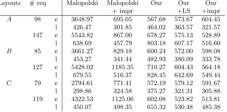
The travel times in Table 4 are not merely the travel distances divided by the speed of the vehicles, because they include all the delays caused by waiting.
This is why the loaded travel times can be shorter in case of our method than that of the Malopolski mehtod, even if the loaded travel distances are always shorter in case of the Malopolski method. The reason for this phenomenon is due to our strategy of deleting all routes first before scheduling new requests into the schedule, see Section 4. Notice also the very significant improvement in the travel times in case of the ’Malopolski+impr’ method. In particular, the empty travel times become much shorter, because the Improve Schedule procedure in many cases cuts back the empty travel to the depot node and unifies it with the route to the pickup station of the next request of a vehicle. However, even after the improvement, the Malopolski method still requires significantly more empty travel time than our method.
We have introduced a new measure that can describe the operation of a sys- tem during the time horizon more accurately. For each instance, we partitioned the requests into 10 (almost) equal size sets Di ⊂ R (i = 1, . . . ,10) by the deciles of the set of pickup times (a number which is not smaller than (10·i)%
of the elements of the set {er : r ∈ R}, but not larger than (100−10·i)%
of the elements of the set). For each Di, we determine the average lateness (P
r∈Di(tr−dr)/|Di|, where tr is the finish time of r), and then, we take the average over the 100 instances. This measure shows how the average lateness changes during the time horizon, and it is able to give a good guess on the average lateness, if the time horizon is longer (and the rate of the number of the
Table 3: Travel distances: average values over 100 instances of the average empty (e), and loaded (l) travel distances of the vehicles.
Layouts # req Malopolski Malopolski Our Our Our
+ impr +LS +impr
A 98 e 506.15 485.18 399.72 402.62 371.15
l 292.68 292.68 366.56 349.28 311.86
147 e 754.93 675.74 540.02 522.53 473.41
l 440.02 440.02 596.35 569.20 490.61
B 85 e 570.40 497.25 410.98 415.20 387.32
l 289.31 289.31 360.60 348.17 311.75
127 e 847.16 719.47 549.27 534.16 495.47
l 430.07 430.07 583.42 563.68 486.74
C 79 e 468.13 415.15 323.55 320.52 309.56
l 278.94 278.94 308.82 304.41 291.90
119 e 702.66 612.41 452.59 446.73 431.53
l 420.02 420.02 497.29 488.25 450.83
Table 4: Travel times: average values over 100 instances of the average empty (e), and loaded (l) travel times of the vehicles.
Layouts # req Malopolski Malopolski Our Our Our
+ impr +LS +impr
A 98 e 3648.97 695.05 567.68 573.67 604.45
l 426.47 301.85 464.02 363.57 321.57 147 e 5543.82 867.00 678.27 575.13 528.89 l 638.69 457.79 803.18 607.17 516.60
B 85 e 3661.27 829.18 600.24 572.00 598.08
l 453.27 341.44 482.93 380.09 333.78 127 e 5428.02 1185.35 710.27 604.43 564.18 l 679.55 516.37 828.45 642.69 549.44
C 79 e 2794.61 771.41 572.19 579.12 591.67
l 298.86 324.58 375.27 321.31 305.88 119 e 4322.53 1125.06 602.08 523.82 513.81 l 450.07 498.35 655.32 530.48 485.38
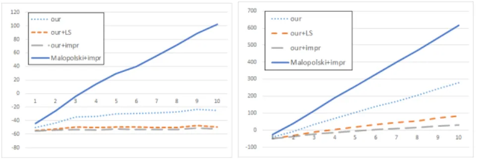
requests, and the length of the time horizon does not change). Figure 9 depicts the results for layoutC, but similar figures could be depicted for the other two layouts as well.
The 10 points on the horizontal axis corresponds to D1, . . . , D10, and the figure depicts the average of average lateness of the requests in Di over 100 instances for different solution methods. The figure does not depict the results of the method of Malopolski without improvements, because it would obscure the differences among the other solution methods. In case of 79 requests, we can see that our method is able handle them even without local search. If we do not use local search then the system needs the extra 60 time units to finish the requests on time, however, approximately 10 time units are enough, if we apply the local search heuristic as well. In contrast, for the Malopolski method
Figure 9: The average lateness ofD1, . . . , D10in case of layoutCand 79 requests (left), and 119 requests (right).
with improvements, the unserved requests accumulate as the time passes, which leads to increasing delays (i.e., the system is overloaded).
For the benchmark instances with 119 requests, the system is overloaded for each method, since the delays increase as the time passes. Observe the difference in the steepness of the curves: this indicates how fast the number of the unserved request increases at any moment.
6 Final remarks
In this paper we have summarized our method for suboptimal and conflict- free AGV control. Our solution is suboptimal for the total tardiness objective function with respect to the due dates of the requests served by the vehicles. It is conflict-free, since under mild assumption, it guarantees that all vehicles can serve their requests. We have performed a series of experiments to assess the performance of the method, and compared it to another complete method from the literature, proposed quite recently. We emphasize that the transportation requests are not known in advance, but they arrive on-line. There are three main novelties in our approach: (i) the planning of the routes of the vehicles already ensures a conflict-free execution, provided the vehicles follow the plan, (ii) the schedule improvement strategies that can significantly decrease the travel distances and delays, and (iii) the consideration of conflict-free routing and the minimum tardiness objective together, in the same problem. The very low computational time of our method indicates that it can scale up well with the size of the problem.
As a continuation, we want to extend our method to vehicles of capacity more than one, i.e., a vehicle may visit a number of different pickup points before delivering an item, the only limitation is its capacity. However, in such a problem, task assignment is even more important, and there is no generally accepted good method for the online multiple pickup and delivery problem with vehicle capacities.