A Heuristic Active Fault Tolerant Controller for the Stabilization of Spacecraft

A Heuristic Active Fault Tolerant Controller for the Stabilization of Spacecraft

Rouzbeh Moradi

¹

, Mohsen Fathi Jegarkandi

²

and Alireza Alikhani

³

1 Aerospace Research Institute (Ministry of Science, Research and Technology), P. o. Box: 14665-834, Tehran, Iran, rouzbeh_moradi@ari.ac.ir

2 Department of Aerospace Engineering, Sharif University of Technology, P. o.

Box: 11365-11155, Tehran, Iran, corresponding author, fathi@sharif.edu

3 Aerospace Research Institute (Ministry of Science, Research and Technology), P. o. Box: 14665-834, Tehran, Iran, aalikhani@ari.ac.ir

Abstract: A heuristic active fault tolerant controller is designed based on the model of elections in a two-party democratic society. The goal of the proposed controller is to modify reference trajectories to maintain the stability of the faulty spacecraft. The elections are assumed to be first order Markovian. Final state constraints are used to ensure that the angular velocities asymptotically converge to the origin. A simulation shows that the proposed method makes the origin an asymptotically stable equilibrium point for the considered spacecraft. Because of its computational efficiency, the proposed method can be effectively used on-line in real-time, an important feature of any active fault tolerant controller. The present paper shows that socio-political models have a great potential to solve complex engineering problems and opens a new window for further developments in this field.

Keywords: Active fault tolerant control, two-party democratic society, reference trajectory management, under-actuated spacecraft

1 Introduction

Fault Tolerant Control (FTC) is an active research area in automatic control theory. The importance of FTC comes from the fact that the conventional feedback control systems are not capable of handling component malfunctions [12]. An almost countless number of books, review papers, research papers and theses have been published in the literature to cover an aspect of this important problem. [11] is a review paper that studies recent developments in the spacecraft attitude fault tolerant control system.

FTC is divided into two main parts: Active FTC (AFTC) and Passive FTC (PFTC). AFTC uses the on-line information provided by fault detection and diagnosis (FDD) to reconfigure the controller after the occurrence of a fault/failure in the system. In PFTC, a robust control method is used to make the closed-loop system as insensitive as possible to a range of anticipated faults and contrary to AFTC, there are no FDD and reconfiguration mechanisms. Therefore, the goal of designing PFTC is to provide a fixed structure controller such that the closed-loop system shows the least sensitivity to anticipated faults in the design stage.

According to this classification, the presence of FDD and a mechanism to reconfigure the controller are two main features distinguishing AFTC from PFTC [12].

Reference trajectory management (RTM) is one of the components of general active fault tolerant controller [12]. The responsibility of RTM [2] is to adjust the reference trajectories, to make the post-fault model of the system stable, even after the occurrence of multiple actuator faults [4].

This paper proposes a heuristic AFTC that is based on the model of elections in a two-party democratic society [8]. Then, the proposed method is used to design an RTM block for a faulty spacecraft. The RTM produces desired reference trajectories to make the origin an asymptotically stable equilibrium point for the post-fault model. The main assumption of the paper is that two-party democratic societies are more stable than the other political systems [8].

A combination of global and local search optimization is used to satisfy the final state constraints. Due to its simple structure, the proposed method has a very low computational complexity and is suitable for on-line and real-time purposes.

The main contribution of this paper is to use socio-political models to solve engineering control problems. To the authors' best knowledge, previous studies have not considered such a methodology. The results show that the main idea has great potential for further research in the future.

This paper consists of the following sections: Section 2 presents the general scheme of the closed-loop system, an introduction to the election process in two- party democratic societies and finally, modeling the election process. Section 3 discusses the rotational dynamics of a rigid spacecraft and the controller structure.

Asymptotic stability is discussed in section 4. Section 5 presents numerical results, and finally, the paper ends with a conclusion.

2 RTM Structure

2.1 The Closed-Loop System

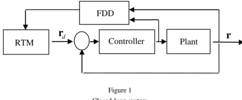
The goal of the proposed RTM is to generate the desired reference trajectories (r_d) to make the origin an asymptotically stable equilibrium point for the post- fault system. Fig. 1 shows the general scheme of the closed-loop system:

Figure 1 Closed-loop system

It is assumed that the post-fault model of the system is provided by the FDD. The desired reference trajectory vector should steer the post-fault model to the origin, even after occurrence of severe actuator faults/failures.

2.2 An Introduction to the Election Process in Two-Party Democratic Societies

The election system in two-party democratic societies is the basis of the proposed RTM. [8] states that two-party democracies tend to be more stable than the other political systems. On the other hand, there is historical evidence that the countries with multi-party democracies are also converging to two-party political systems [1].

One of the main features of a two-party system is as follows: if a destabilizing effect occurs in the society, e.g. a war or economic crisis, the opposition party will be selected by the public [8].

According to [10], it is possible to map any political spectrum to the left-right axes. This paper suggests Fig. 2 as a possible mapping:

Controller Plant RTM

FDD

r

d

_r

Figure 2

Political spectrum in the response diagram

Fig. 2 shows the upper and lower bounds of the conservative and radical policies.

There is a total of four bounds that define the boundaries of the political spectrum.

However, since RLLB = CLUB and RRLB = CRUB (Fig. 2), the total number of bounds for a state is reduced to two.

A conservative policy adheres to tradition and opposes any radical social change [7]. According to this definition, a conservative policy (whether it belongs to the left or right parties) favors being close to the equilibrium. The opposite is true about radical policies.

These facts are the basis of three important claims in this paper:

a) In a fast converging society, the public is satisfied with the ruling party and votes for the conservative policies.

b) In a moderately converging society, the public votes for the current policies.

c) In a slowly converging/diverging society, the public votes for the opposition party.

Assumption 1: The elections are assumed to be first order Markovian. In other words, the result of the current election is only dependent on the result of the previous election. This assumption is directly adopted from [8].

Left

Right

Radical

Conservative

Radical Right (RR) Conservative Left (CL)

Conservative Right (CR) t t1

t t2

t t3

t t4

Radical Left (RL) Conservative

Radical

Radical Left Lower Bound (RLLB) Conservative Left Upper Bound (CLUB)

Radical Right Lower Bound (RRLB) Conservative Right Upper Bound (CRUB)

2.2 Modeling the Election Process

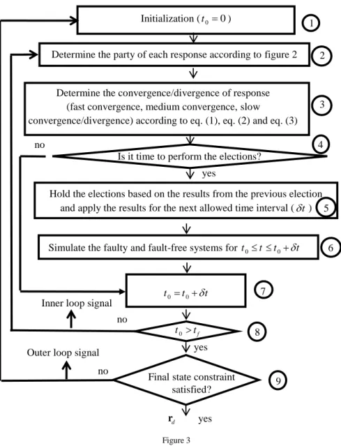
Fig. 3 shows the general scheme of the election process:

Figure 3

General scheme of the proposed method

This flowchart consists of two loops: an inner loop and an outer loop. According to Fig. 3, a description of the procedure is as follows:

Initialization (t₀0)

Determine the party of each response according to figure 2

Hold the elections based on the results from the previous election and apply the results for the next allowed time interval (t )

0 0

t   t t t free systems for

- Simulate the faulty and fault

Inner loop signal

Outer loop signal

Determine the convergence/divergence of response (fast convergence, medium convergence, slow

convergence/divergence) according to eq. (1), eq. (2) and eq. (3) no

yes

0 0

t  t t

0 f

t t yes no

yes

1 2

3

4

5

7

8

9 Is it time to perform the elections?

Final state constraint satisfied?

no

rd

6

3

1-The initial conditions, the election parameters (to be defined in this section) and the controller parameters are defined, and t₀ is set to zero.

2-The party of each state is determined, according to Fig. 2.

3-After determining parties, the regime of states is evaluated. Three main regimes are considered: fast convergence, medium convergence, slow convergence/divergence.

These regimes are determined according to the following criteria (where x_i and

ni

x are the i-th components of the faulty and nominal (fault-free) state vectors, respectively):

Fast convergence:



0

 

0



1

 

0

 

0 1

1 1

0 1

i i

n n

i n i n

i i

x t t x t t  x t x t 

 

      

 

⁽¹⁾

1 is the fast convergence coefficient and n is the number of states.

Divergence or slow convergence:



0

 

0



2

 

0

 

0 2

1 1

0 1

i i

n n

i n i n

i i

x t t x t t  x t x t 

 

      

 

⁽²⁾

2 is the slow convergence/divergence coefficient and ₂ ₁. Medium convergence:

   

   

   

1 0 0

1

0 0

1

2 0 0

1

i

i

i n

i n

i n

i n

i n

i n

i

x t x t

x t t x t t

x t x t



 









 

   









(3)

4-Is it time to hold an election?

To hold an election, the current time should be smaller than t^* (this parameter will be defined in section 4).

5-If it is allowed, the election is held. The results of the previous election are used to determine the results of the current election (assumption 1). The procedure is as follows:

If the regime of states is "fast convergence"; the desired trajectories become the origin or r_d 0 (the public votes for conservative policies). If the regime of states is "slow convergence/divergence"; the opposition party is elected. If the regime of

states is "medium convergence"; the previous reference trajectories are selected again (the public votes for the current policies).

To make the election process clearer, an example is presented:

Example:

1, ₂ and ₃ are the spacecraft angular velocities (refer to section 3). Assume that ₁ is the least qualified state.

Note 1: A state will be the least qualified if it deviates more than the other states from the fault-free system. Obviously, for under-actuated systems, the un-actuated state will be the least qualified.

In order to stabilize the system, the public votes for the following reforms:

If the policy of ₂ is RR, the party of _d,2 changes to CR (more details will be presented in the following)

If the policy of ₂ is CR, the party of _d,2 changes to CL If the policy of ₂ is CL, the party of _d,2 changes to CR If the policy of ₂ is RL, the party of _d,2 changes to CL

Note 2: If the reforms are carried through rapidly, false conclusions will be made about the performance of the ruling party. Therefore, it is assumed that when the policy of a state is radical, it first switches to conservative and then the opposition party is elected. This is equivalent to gradual reforms in the society.

Note 3: ₂ is selected to carry through the reform and ₃ is used as an assistant for ₂ to perform its policy making. If ₃ does not help ₂, ₂ will be forced to act alone and therefore, the performance will not be acceptable. The role given to the assistant state (₃ in this case), has its roots in the spacecraft dynamics (eq.

(6)).

According to note 3, the following policy makings are also performed by ₃: If the policy of ₃ is RR, it remains there (more details will be given in the following paragraphs)

If the policy of ₃ is CR, the party of _d,3 changes to RR If the policy of ₃ is CL, the party of _d,3 changes to RL If the policy of ₃ is RL, it remains there

In order to quantify the outcome of elections, the following procedures will be considered:

If the next policy is CL/CR (CL or CR), r_d will be the average of zero (origin) and CLUB/CRUB and if the next policy is RL/RR,r_d will be RLLB/RRLB.

Therefore, r_d will be constant in t intervals (refer to the simulation section).

Since the upper and lower bounds are selected as the election parameters (section 4), the whole political spectrum will be covered, and no political censorship will occur.

6-Faulty¹ and nominal (fault-free) systems are simulated for t₀  t t₀ t . 7-t₀ is updated to t₀t .

8-A condition to check whether t₀ t_f , where t₀ and t_f are the current and final times, respectively. If this condition is not satisfied, the inner loop continues from the beginning.

9-The final state constraint (eq. (16)) is checked. If this condition is not satisfied, the outer loop continues from the beginning.

Modeling the election process has now been completed. Spacecraft dynamics and controller structure are the subjects of the next section.

3 Spacecraft Dynamics and Control

3.1 Spacecraft Dynamic Equations

The rigid body spacecraft rotational dynamics in the principal coordinate system is described by the following equations [9]:

2 3

1 1 2 3 1 1

1

3 1

2 2 1 3 2 2

2

1 2

3 3 1 2 3 3

3

J J

u J

J J

u J

J J

u J

    

    

    

  

     

 

  



    

 

  

     

 

(4)

1 - It is assumed that the FDD block provides the post-fault information



  1, 2, 3



are the angular velocities,



u u u1  , 2, 3



are the normalized control inputs and finally,



J J J1, 2, 3



are the principal moments of inertia of the rigid body along the principal body axis. The relation between control torques and inputs are given by the following equations:

1 1 1

2 2 2

3 3 3

u u J

u u J

u u J

 

 

 

(5)



u u u1, 2, 3



are the three control moments acting on the spacecraft. The upper and lower bounds of the control inputs are restricted according to the following saturation function:

 

max ^max max^max

max max

if

sat if

if

i i

i i

i

u u u u

u u u u

u u u

  



 

   



(6)

umax is the maximum torque that can be produced by the actuators.

3.2 Controller Structure

The error signal is defined as follows:

e   d

ω ω ω (7)

ωd and ω_e are the desired and error angular velocity vectors, respectively.

Rewriting the spacecraft dynamics in the form of error dynamics will result in the following set of equations:

  

  

  

1 1 1 1 2 2 3 3 1 1 1

2 2 2 2 1 1 3 3 2 2 2

3 3 3 3 1 1 2 2 3 3 3

e d e d e d d

e d e d e d d

e d e d e d d

u u

u u

u u

        

        

        

 

       

 

       

 

       

(8)

The nonlinear terms are canceled using feedback linearization. Consequently, the closed-loop system will be transformed into the following simple linear time invariant form:

1 1

2 2

3 3

e e e

u u u







 

 

 

(9)

and the following form of feedbacks will lead to the exponential stabilization of ωe to zero:

 

 

 

1 1 1 1

2 2 2 2

3 3 3 3

e e e

u k k R

u k k R

u k k R













   

   

   

(10)

This will result in the exponential convergence of ω to ω_d .

Considering the set of eq. (8) and eq. (10),



u u u1  , 2, 3



will be obtained as follows:

  

  

  

1 1 2 2 3 3 1 1 1

2 2 1 1 3 3 2 2 2

3 3 1 1 2 2 3 3 3

e d e d d e

e d e d d e

e d e d d e

u k

u k

u k

      

      

      

      

      

      

(11)

For feedback purposes, it is more suitable to rewrite



u u u1  , 2, 3



in terms of the original variables:

    

     

    

1 1 2 3 1 1 1 1

2 2 1 3 2 2 2 2

3 3 1 2 3 3 3 3

d d

d d

d d

u k

u k

u k

     

     

     

     

     

     

(12)

These are the desired control inputs that will lead to the exponential convergence of ω to ω_d.

Now imagine ω_d 0. The equations of the closed-loop system will be:

 

 

 

1 1 1

2 2 2

3 3 3

k k k

 

 

 

 

 

 

(13)

Clearly, as long as there is no saturation and the actuators can produce the required control inputs, the closed-loop system remains globally exponentially stable (GES). However, after the occurrence of actuator failures, GES will not be guaranteed. As will be seen in the simulation section, the proposed method will be able to steer the faulty system towards the origin. This happens even when severe actuator failures occur, and the system becomes under-actuated.

The next section will provide a stability analysis to prove that under a certain condition, the proposed method can make the origin an asymptotically stable equilibrium point for the faulty system.

4 Stability Analysis

As shown in Fig. 1, the RTM block receives the post-fault model of the system and produces the desired reference trajectory vector (r_d). The qualitative and quantitative procedures outlined in Section 2 are the main structures of the RTM block. However, in order to tune the election parameters, the following problem should be solved:

Determine the election parameters (₁,_2, tand political spectrum) such that the final state vector becomes zero, i.e. ω

 

tf ⁰. Such a final state constraint is well-known in the literature and is introduced to ensure asymptotic stability [3].

Note 4: In order to make sure ω_d approaches the origin before t t_f , its value is set to zero as t passes t^*.

In other words:

0 * d   t t

ω (14)

In order to give the solver more flexibility to solve the problem, another variable (k_s) is introduced:

 

* _{s f s} 0.5 1

t k t k  (15)

The role of k_sis to determine t^* as a function of the final time. This will give the solver more flexibility to solve the problem.

Remark 1: The proposed method includes some issues related to the convergence (eq. (1), eq. (2) and eq. (3)). Therefore, as will be seen in the simulation section, the final state constraint can be easily satisfied through a few simulations.

Consequently, the convergence speed will be high (a very important feature of any AFTC design).

5 Simulation

The system/controller parameters and initial conditions are given in Table 1:

Table 1

System/Controller parameters and initial conditions Controller

parameters

Initial

conditions (degree/sec) Moments

of Inertia (kg.m²⁾

k1 0.1  

1 0

 10 J₁ 449.5

k2 0.1 ₂ 0 10 J2 264.6

k3 0.1  

3 0

 -15 J₃ 312.5

It is assumed that the fault occurs at t_fault 10second and the final time is

f 200

t  second.

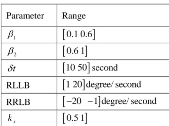
Table 2 presents the range of the election parameters:

Table 2

Range of the election parameters

Parameter Range

1



0.1 0.6



2



0.6 1



t



^{10 50}



^second

RLLB



1 20 degree/ second



RRLB



20 1 degree/ second



ks



0.5 1



In order to satisfy the final state constraint



ω

 

tf ⁰



, eq. (16) is defined:

   

3 2 2

1

0.01 deg/ sec

i f

i

 t





 ⁽¹⁶⁾

A combination of global (Genetic Algorithm¹ [6]) and local (Sequential Quadratic Programming² [5]) optimization is used to satisfy eq. (16). First, GA explores the search space to find the promising region and then SQP exploits the region to satisfy eq. (16). The population size of GA is selected as 20. The other parameters of GA and SQP are the default values considered in MATLAB 2011a. The stopping criteria for GA and SQP are illustrated in Table 3:

1 -GA (ga command)

2 -SQP (fmincon command)

Table 3

Stopping criteria for GA and SQP

GA 500 seconds elapsed time

SQP Satisfying eq. (16)

The actuation system consists of six thrusters (without considering hardware redundancy), that are placed in opposite directions and each thruster is capable of producing a maximum of 50 N variable thrust. The effective moment arm of all thrusters is one meter along the principal body axis. However, the configuration of the thrusters is such that (T1-T2), (T3-T4) and (T5-T6) produce net moments about the first, second and third principal axes, respectively (fig. 4). (Direction of the arrows = Direction of the forces).

Figure 4 Thruster configuration

It seems that the thrusters T3, T4, T5 and T6 pass through CG. However as stated in the previous paragraph, they have a moment arm of one meter along the first body axis.

The considered failure scenario is presented in Table 4:

Table 4 Failure scenario

Failure scenario Failure of T1 and T2 (first body axis is under-actuated) This failure scenario makes the spacecraft under-actuated, a challenging issue for control purposes.

T5 T6

T3

T4

CG

1 2

3

Direction of forces = direction of arrows T2 T1

5.1 Failure Scenario

5.1.1 Without RTM

Fig. 5a and Fig. 5b illustrate the nominal (fault-free) and faulty (without RTM) systems response and control input:

Figure 5a

Nominal and faulty systems response- first fault scenario (without RTM)

Figure 5b

Nominal and faulty systems control input- first fault scenario (without RTM) It is observed that if the faulty system is not recovered, ₁ will not converge to the origin (a previously predicted result).

5.1.2 With RTM

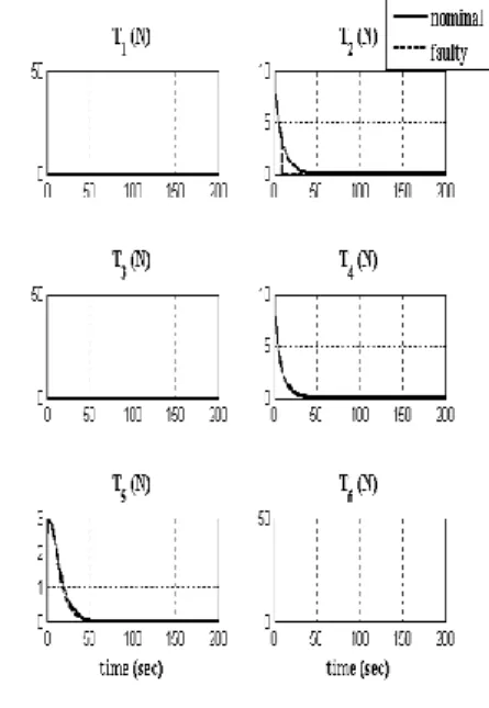
The corrected faulty system response and control input are illustrated in Fig. 6a and Fig. 6b¹:

1 -Intel(R) Core^TM2 CPU, T7200@2.00GHz, MATLAB® 2011a

Figure 6a

Faulty system response (with RTM)-first fault scenario (elapsed time=671sec)

Figure 6b

Faulty system control input (with RTM)-first fault scenario

Remark 2: "desired" signal shown by the dashed line is the modified ω_d, assumed to be constant in t intervals.

A comparison of Fig. 5a and Fig. 6a shows the ability of the proposed method to steer the post-fault system to the origin. Table 5 presents the obtained results for the election parameters:

Table 5

Election parameters obtained for the first fault scenario

1 _0.53

2 0.61

t 46.53

RLLB for ₁ 16.43 degree /sec RRLB for ₁ -8.11 degree /sec RLLB for ₂ 14.42 degree /sec RRLB for ₂ -16.97 degree /sec RLLB for ₃ 11.29 degree /sec RRLB for ₃ -6.76 degree /sec 1

2

In order to explain the election process, two dashed ellipses are shown in Fig. 6a.

Circle 1 demonstrates a reform. As mentioned in the text, the reason for such an election is the slow convergence/divergence of states. Circle 2 shows the election of conservative policies. This election shows that the public is satisfied with the fast rate of convergence.

Note 5: According to the simulation results and the elapsed time, the proposed method is real-time (refer to http://stackoverflow.com/questions/20513071/ for more information).

Remark 3: One of the limitations of the proposed RTM is that the desired reference trajectories are considered to be constant in t intervals. Future work will concentrate on more flexible trajectory generation tools, like cubic splines.

This idea will make the proposed RTM more applicable to a wider class of systems.

One of the main contributions of this paper is to use political theories to solve control problems. To the authors' best knowledge, no previous work has considered such methodology. The results show that the proposed method has a great potential for further developments.

Note 6: The present paper shows that socio-political models have a great potential to solve complex engineering problems. On the other hand, implementation of such ideas in engineering applications can be used as a method for their evaluation. Such a bilateral relationship will be helpful for both socio-political and engineering related problems.

Conclusions

Based on the model of elections in two-party democratic societies, a heuristic RTM for AFTC was proposed. The proposed method was implemented on a spacecraft, and it was observed that the faulty system was able to reach the origin, an event that would not occur if no actions were taken. The present paper shows the ability of socio-political models to solve complex engineering problems and opens a new window for further developments in this field.

References

[1] Aloisi, S: Election pushes Italy towards two-party system, Reuters, http://www.reuters.com/article/us-italy-election-system-

dUSL1580537620080415, accessed 1 November 2016

[2] Nemes, A: Continuous Periodic Fuzzy-Logic Systems and Smooth Trajectory Planning for Multi-Rotor Dynamic Modeling, Acta Polytechnica Hungarica, Vol. 13, No. 6 (2016)

[3] Fontes, FACC: A general framework to design stabilizing nonlinear model predictive controllers, Systems and Control Letters, doi:10.1016/S0167- 6911(00)00084-0 (2001)

[4] Garone, E., Cairano, S. Di and Kolmanovsky, I. V: Reference and command governors for systems with constraints: A survey on theory and applications, Mitsubishi Electric Research Laboratories, http://www.merl.com (2016)

[5] Gill, PE., Murray, W and Wright, MH: Practical Optimization, Emerald Group Publishing Limited, ISBN-13: 978-0122839528 (1982)

[6] Goldberg, DE: Genetic Algorithms in Search, Optimization & Machine Learning, Addison-Wesley Professional, 1 edition, ISBN-13: 978- 0201157673 (1989)

[7] McLean, I and McMillan, A: Conservatism: Concise Oxford Dictionary of Politics, Oxford University Press, Third Edition, ISBN: 978-0-19-920516-5 (2009)

[8] Midlarsky, MI: Political stability of two-party and multi-party systems:

probabilistic bases for the comparison of party systems, The American Political Science Review, doi: 10.2307/1955799 (1984)

[9] Sidi, MJ: Spacecraft Dynamics and Control: A Practical Engineering Approach, Cambridge University Press, Revised edition, ISBN-13: 978- 0521787802 (2000)

[10] Ware, A: Political Parties and Party Systems, Oxford University Press, ISBN: 9780198780779 (1995)

[11] Yin, S., Xiao, B., Ding, S and Zhou, D: A review on recent development of spacecraft attitude fault tolerant control system, IEEE Transactions on Industrial Electronics, 63(5): 3311-3320, doi: 10.1109/TIE.2016.2530789 (2016)

[12] Zhang, Y and Jiang, J: Bibliographical review on reconfigurable fault-

tolerant control, Annual Reviews in Control,

doi:10.1016/j.arcontrol.2008.03.008 (2008)