Additive Main Effects and Multiplicative Interaction and Yield Stability Index for Genotype by Environment Analysis and
Wider Adaptability in Barley
V. Kumar*, a.S. Kharub and G.P. SinGh
ICAR-Indian Institute of Wheat & Barley Research, Karnal-132001 (HR) (Received 4 May 2017; Accepted 11 October 2017;
Communicated by V. Korzun)
Genotype by environment interaction distorts genetic analysis, changes relative ranking of genotypes and a major obstruction for varietal release. AMMI model is a quick and rele- vant tool to judge environmental behaviour and genotypic stability in comparison to ANOVA, multiplicative model and linear regressions. We evaluated 19 barley genotypes grown at 08 diverse locations to identify discriminating environments and ideal genotypes with dynamic stability. In AMMI ANOVA, the locations and genotype by environment inter- action exhibited 66% and 14.7% of the total variation. The initial first two principal compo- nents showed significant interaction with 36.0 and 28.4% variation, respectively. AMMI1 biplot showed that the environments Bawal, Ludhiana and Durgapura were high yielding with high IPCA1 scores and located far away from the biplot origin. However, in AMMI1and AMMI2 biplots the locations Hisar, Ludhiana, Karnal, Bathinda and Modipuram were found suitable with low IPCA2 scores. Yield stability index (YSI) was highly useful with ASV ranks and the genotypes DWRB150 and BH1013 and checks BH902, DWRUB52 and DWRB101 were selected for high grain yield and wider adaptability across the locations.
Keywords: AMMI, ASV, YSI, G×E, barley
Introduction
Barley is one of the most important and ancient crop species. The archaeological evi- dences have been revealed that the crop was domesticated 10000 years ago with other crops like wheat, lentil and pea in the “Fertile Crescent” of the Middle East (Baik and Ullrich 2008). Barley is very much genetically diverse crop and historically known to be used by warriors and gladiators. The crop is mainly used for food and feed purposes in developing countries and has also evolved for malting and brewing due to its enzymatic activities and husk content in developed world (Kumar et al. 2013; Kumar et al. 2014).
During 2014, barley ranked fourth among cereals and occupied 49.42 m ha area and pro- duced 144.48 m t grains after wheat (220 m ha and 729 m t), maize (184.8 m ha and 1037.8 m t) and rice (162.7 m ha and 741.5 m t), respectively (FAOSTAT 2017). World- wide, Asia produced 17.75 m t (13.56%) barley grain from 11.02 m ha land (22.3%) with below worlds average productivity of 19.56 q/ha. Out of South-Asian grain production of
*Corresponding author; E-mail: vishnupbg@gmail.com
5.25 m t, India contributed 34.86% grain production with 27.15 q/ha productivity, respec- tively. Barley is a versatile diploid crop species, which thrives well under drought, salin- ity and alkalinity and requires lower input than other winter (rabi) cereals like wheat. The crop is being grown under diverse agro-ecologies i.e. from rainfed areas of northern hills, north eastern plains to high-input conditions of northern Indo-Gangetic plains in India.
Presence of several multi-national malting and brewing industries has further opened up new frontiers for barley research, production and demand in India.
Genotype by environment interaction (G×E) still stands one of the major complica- tions in the genetic analyses and on farm yield maximization (Crossa et al. 2012). Agri- cultural science has much progressed in crop production, protection and biotechnological tools but yield continued to be the first and foremost objective for food security. Yield is a complex trait and highly influenced by G x E, which ultimately hampers potential yield realization at farmers field. The physical and biological surroundings of the plant canopy leads many changes in plant responses and especially varying soil and weather properties further aggravates this situation across the locations. The genotype by environment inter- action influences the genotype performances to a greater extent that even a top ranking genotype may be the poor yielding at another location leaving breeder helpless. This in- consistent performance and changed relative ranking of the genotypes needed plant breeder’s attention and challenged to apply an easy, efficient, quick tool to identify high yielding genotypes with wider adaptability across the environments (Asfaw et al. 2009;
Mohammadi and Amri 2013; Kuchanur et al. 2015).
Becker and Leon 1988; Flores et al. 1998 reviewed and reported different stability models based on analysis of variance, multivariate models, linear regressions (Finlay and Wilkinson 1963; Eberhart and Russell 1966) etc. Flores et al. 1998 further categorised these models for stability, yield and stability and yield only (Alwala et al. 2010). Whereas, Becker and Leon 1988 very well classified stability models for parametric, non-paramet- ric and multivariate approaches. Rakshit et al. 2012; Mohammadi and Amri et al. 2013 reported that ANOVA is an additive model and emphasizes main effects, while multipli- cative models mainly focus the interaction effects. The Additive Main Effects and Multi- plicative Interaction (AMMI) is a biplot based graphical unique linear-bilinear model and combines both of the above approaches of ANOVA and multiplicative models (Gabriel 1971; Gauch 1988; Yan et al. 2007). AMMI model is an efficient method to study stable genotypes and discriminating environments and widely used in several studies (Nurmin- iemi et al. 2002; Mortazavian et al. 2014; Sousa et al. 2015; Raggi et al. 2017; Rakshit et al. 2017). It displays main effects, environment (E) main effects, and genotype by envi- ronment interaction effects on a biplot and helpful for the plant scientists to see and judge desirable genotypes and environments (Gauch 2006; Gauch et al. 2008). Moreover, the concepts of AMMI stability value and yield stability index (YSI) further substantiate the AMMI analysis for selecting high yielding genotypes with dynamic stability. Unfortu- nately, the information pertaining to environmental behaviour for barley is scanty in India and vast zonation further makes problem serious during varietal release. Keeping in mind the above facts, the AMMI analysis with ASV and YSI was carried to delineate the dis- criminating environments and stable genotypes with wider adaptability in barley.
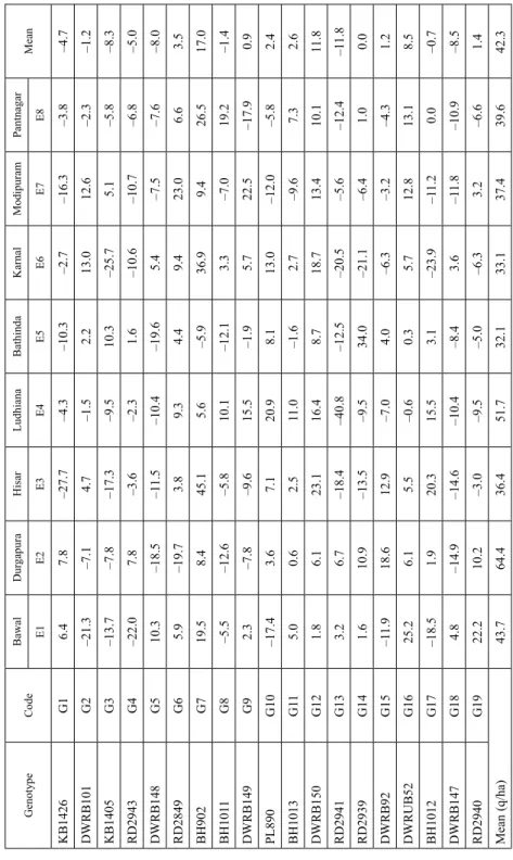
Table 1. Per cent performance for genotypic grain yield relative to the each location mean (q/ha) at the multi-locations GenotypeCodeBawalDurgapuraHisarLudhianaBathindaKarnalModipuramPantnagar Mean E1E2E3E4E5E6E7E8 KB1426G16.47.8–27.7–4.3–10.3–2.7–16.3–3.8–4.7 DWRB101G2–21.3–7.14.7–1.52.213.012.6–2.3–1.2 KB1405G3–13.7–7.8–17.3–9.510.3–25.75.1–5.8–8.3 RD2943G4–22.07.8–3.6–2.31.6–10.6–10.7–6.8–5.0 DWRB148G510.3–18.5–11.5–10.4–19.65.4–7.5–7.6–8.0 RD2849G65.9–19.73.89.34.49.423.06.63.5 BH902G719.58.445.15.6–5.936.99.426.517.0 BH1011G8–5.5–12.6–5.810.1–12.13.3–7.019.2–1.4 DWRB149G92.3–7.8–9.615.5–1.95.722.5–17.90.9 PL890G10–17.43.67.120.98.113.0–12.0–5.82.4 BH1013G115.00.62.511.0–1.62.7–9.67.32.6 DWRB150G121.86.123.116.48.718.713.410.111.8 RD2941G133.26.7–18.4–40.8–12.5–20.5–5.6–12.4–11.8 RD2939G141.610.9–13.5–9.534.0–21.1–6.41.00.0 DWRB92G15–11.918.612.9–7.04.0–6.3–3.2–4.31.2 DWRUB52G1625.26.15.5–0.60.35.712.813.18.5 BH1012G17–18.51.920.315.53.1–23.9–11.20.0–0.7 DWRB147G184.8–14.9–14.6–10.4–8.43.6–11.8–10.9–8.5 RD2940G1922.210.2–3.0–9.5–5.0–6.33.2–6.61.4 Mean (q/ha)43.764.436.451.732.133.137.439.642.3
Material and Methods
To perform AMMI 1 and AMMI 2 analyses, multi-location yield trials were conducted at 8 diverse locations namely, Bawal (E1), Durgapura (E2), Hisar (E3), Ludhiana (E4), Bathinda (E5), Karnal (E6), Modipuram (E7) and Pantnagar (E8) during rabi, 2015-16.
The experimental material comprised of 19 barley genotypes viz. KB1426 (G1), DWRB101 (G2), KB1405 (G3), RD2943 (G4), DWRB148 (G5), RD2849 (G6), BH902 (G7), BH1011 (G8), DWRB149 (G9), PL890 (G10), BH1013 (G11), DWRB150 (G12), RD2941 (G13), RD2939 (G14) DWRB92 (G15), DWRUB52 (G16), BH1012 (G17), DWRB147 (G18) and RD2940 (G19) (Table 1). Out of the above experimental materials, the genotypes G2, G6, G7, G15 and G16 were the commercial checks. The experiments were conducted in randomized complete block design (RCBD) with four replications of 6-row plots in each environment with 5 m row length and spaced 18 cm apart, respec- tively. Recommended crop production and protection package and practices were fol- lowed to raise the good crop. Analysis of variance was carried out using SAS version 9.3 and the AMMI analysis was carried out using R version 3.3.2. The AMMI model is dou- bly centred PCA and written as (Gauch 2006; Gauch et al. 2008):
Yijr – αi – βj + μ = Σnλnγinδjn + ρij + εijr (1) Where, Yijr is the yield of genotype (i) in environment (j) for replicate r, μ is the grand mean, αi represents genotype deviation, βj denotes environment deviation, λn is singular value for component n, γin is the eigenvector value for i, δjn is the eigen vector value for j, the residual is ρij and εijr is the error for genotype i, environment j and replicate r.
AMMI stability value (ASV)
The AMMI stability value (ASV) values were computed as per Purchase et al. 2000; Rad et al. 2013):
ASV= √[(SSIPCA1/SSIPCA2)(IPCA1)2] + (IPCA2)2 (2) Where (2), SSIPCA1 and SSIPCA2 are sum of squares of IPCA1 and IPCA2, respec- tively and IPCA1 and IPCA2 are the genotypic scores in the AMMI model.
Yield stability index (YSI)
Based on ranks of AMMI stability value (RASV) and overall yield (Ry) the yield stability index was calculated as (Oliveira et al. 2014)
YSI = RASV + Ry (3)
Results
The pooled analysis of variance exhibited significant differences for genotypes (G), loca- tions (L) and genotype x location interactions (G×L) and indicated the differential re- sponse of the genotypes across the locations.
This inconsistent performance of the genotypes coupled with significant genotype by locations mean squares further directed of changed relative ranking and crossover G×E across the locations. The locations and genotype by environment interactions contributed 66% and 14.7% of the total variation, whereas the genotypes attributed only 5.6% of the total sum of squares, respectively (Table 2). The situation substantiated for significant
Table 2. Analysis of variance for additive main effects and multiplicative interactions of 19 genotypes
Source DF Type III SS Mean Square Pr > F
Location 7 63308.74 9044.10 <.0001
Rep(loc) 24 1334.28 55.59 0.001
Genotype 18 5285.31 293.62 0.0008
Loc*Geno 126 13955.95 110.76 <.0001
PC1 24 5026.93 209.46 <.0001
PC2 22 3957.91 179.90 <.0001
PC3 20 1960.81 98.04 <.0001
Residual 60 3010.30 50.17 <.0001
Error 432 11161.71 25.83
Total 607 95046.01 R-sq.=0.88 √MSE=5.08
Figure 1. Triangular view of initial three principal components in barley
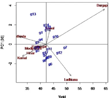
Figure 2. AMMI1 biplot based on additive main effects vs. PC1
Figure 3. AMMI2 biplot based on initial two principal components
role of the locations in changed genotypic ranks and warranted to apply some rigid and easy stability model to comprehend G x E interactions with adaptable cultivars. Location wise, the highest mean grain yield was depicted at Durgapura (64.4 q/ha) followed by Ludhiana (51.7 q/ha) and Bawal (43.7 q/ha). The high yielding genotypes were recorded as BH902 followed by DWRB150, DWRUB52, RD2849 etc. (Table 1).
In AMMI ANOVA the overall treatment mean squares (g + l + gl) explained significant variation (86.3%) of the total mean squares. Besides, additive main effects the genotype by environment interactions were further partitioned into multiplicative interaction prin- cipal components and first 03 PCs exhibited significant interaction with 36.0, 28.4 and 14.1% variation, respectively (Fig. 1). The triangular view of initial three PCs suggested scattered pattern for the genotypes and the environments. Based on the three principal components the locations Bawal and Modipuram were classified altogether, while Dur- gapura showed differential behaviour.
In the present analysis, AMMI1 graph was obtained by plotting genotypic main effects on the absicca vs. first principal component scores (IPCA1) on the ordinate (Fig. 2). The biplot generated for AMMI1 depicted that the environments Bawal, Ludhiana and Dur- gapura were high yielding locations with high additive genotypic main effects, while rest
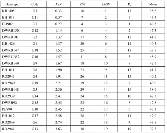
Table 3. AMMI stability values (ASV), yield stability index (YSI) and grain yield (q/ha) for 19 genotypes in barley
Genotype Code ASV YSI RASV Ry Mean
KB1405 G3 0.33 18 1 17 38.8
BH1013 G11 0.57 7 2 5 43.4
BH902 G7 0.77 4 3 1 49.5
DWRB150 G12 1.14 6 4 2 47.3
DWRB101 G2 1.32 17 5 12 41.8
KB1426 G1 1.37 20 6 14 40.3
DWRB147 G18 1.52 25 7 18 38.7
DWRUB52 G16 1.57 11 8 3 45.9
DWRB149 G9 1.67 18 10 9 42.7
BH1011 G8 1.90 23 9 13 41.7
RD2943 G4 1.91 26 11 15 40.2
RD2940 G19 2.21 19 12 7 43.0
DWRB148 G5 2.30 29 14 16 38.9
RD2939 G14 2.41 24 15 10 42.3
DWRB92 G15 2.45 23 16 8 42.8
PL890 G10 2.45 22 17 6 43.3
BH1012 G17 2.58 28 13 11 42.0
RD2849 G6 2.74 22 18 4 43.8
RD2941 G13 3.63 38 19 19 37.3
of the environments were below than the environmental mean. Based on the genotypic grain yield response the locations namely, Karnal, Hisar, Modipuram and Pantnagar were grouped near to each other.
The AMMI2 biplot was also constructed by plotting two initial components i.e. IPC1 and IPCA2 scores on the absicca and ordinates, respectively (Fig. 3). The AMMI2 biplot again confirmed that the environments Bawal, Ludhiana and Durgapura were discrimi- nating and located far away from the origin with long vectors. The locations Hisar, Ludhi- ana, Karnal, Bathinda and Modipuram were found suitable based on IPCA1 and IPCA2 scores. The scattered pattern of AMMI1 biplot represented that the genotypes namely, G7 (BH902), G11 (BH1013), G12 (DWRB150) and G16 (DWRUB52) depicted high mean grain yield. Based on AMMI2 biplot the genotypes G2 (DWRB101), G3 (KB1405), G7 (BH902), G11 (BH1013) and G12 (DWRB150) were located near to the biplot origin and found stable.
In addition to AMMI1 and AMMI2 models the AMMI stability Values (ASV) were calculated to identify stable and ideal genotypes (Table 3). The results obtained for ASV exhibited that the genotypes G3 (KB1405-0.33) followed by G11 (BH1013-0.57), G7 (BH902-0.77), G12 (DWRB150-1.14), G2 (DWRB101-1.32) etc. were found with low ASV. Moreover, based upon the yield stability index (YSI) scores the genotypes viz., BH902 (4) followed by DWRB150 (6), BH1013 (7), DWRUB52 (11) and DWRB101 (17) were selected with low ASV coupled with high grain yield across the locations.
Discussion
Barley is an important coarse cereal being utilized as food, feed and malting and brewing purposes. The inherent tolerance for drought and salinity/alkalinity further favours crop to be taken under cultivation especially by small and marginal farmers. Genotype by en- vironment interaction (G×E) confounds with genotypic main effects (P = G + E + GE) and changes relative ranking of the genotypes (Kumar et al. 2016a). Thus for yield maxi- mization a genotype with higher yield should also follow the dynamic stability as elabo- rated by Becker and Leon 1988. Here, we applied the AMMI model to ascertain the high yielding and stable genotypes and to find out discriminating environments in barley. The combined analysis of variance depicted significant mean squares for genotypes, locations and genotype by location interactions, where locations attributed 66.7% of the total vari- ation. The significant G×E was further partitioned in AMMI ANOVA and showed signifi- cant principal components IPCA1, IPCA2 and IPCA3 with 36, 28.4 and 14.1% variation, respectively.
AMMI model is fixed effect method and considering genotypes and locations as fixed effects was applied here over 19 barley genotypes grown across 08 locations. Edaphic and weather are two main factors and can be considered as fixed effects due to constant soil properties and predictable weather for a particular location in a year (Rakshit et al. 2012).
In AMMI1 and AMMI2 models the locations namely Bawal, Ludhiana and Durgapura were exhibited discriminating with high IPCA1 scores and also located far away from the biplot origin. It is also evident in Table 1 and location means further substantiated that
these locations were responsive. However, while considering IPCA1 and IPCA2 scores the locations Karnal, Modipuram, Bathinda, Hisar and Ludhiana were best suited for genotypic evaluation. Rakshit et al. 2012; Mohhamad and Amri 2013; Kumar et al. 2016b also described that the locations with high IPCA1 scores and low IPCA2 scores are better for genotypic evaluation. Similarly, the genotypes with low IPCA2 scores and near to biplot origin are considered as stable in AMMI2 model and high main effects of these genotypes can be further confirmed from AMMI1 biplot. Therefore, the genotypes G7 (BH902), G11 (BH1013) and G12 (DWRB150) were regarded as high yielding and stable genotypes. The genotype KB1405 (G3) was also located near to biplot origin but found poor yielder.
The above genotypes namely BH902, DWRB150 and BH1013 are in line of the dy- namic stability concept as described by Becker and Leon 1988, which is mainly required for quantitative traits. Moreover, to quantify and substantiate AMMI1 and AMMI2 results the AMMI stability values (ASV) and yield stability index (YSI) were also calculated.
Purchase et al. 2002 reported that the ASV is the distance of the varieties from the biplot origin in respect to the IPCA1 and IPCA2 scores. Based on ASV the genotypes KB1405, BH1013, BH902, DWRB150 and DWRB101 were found stable with low ASV. It has been reported by Oliveira et al. 2014 that in addition to the ASV the yield stability index (YSI) is more efficient criterion, which simultaneously considers stability and yield rank into the single index. Here, we found that the genotypes BH902, DWRB150, BH1013, DWRUB52 and DWRB101 showed low yield stability index and found high yielding and as well as stable. The YSI index was observed more pertinent to identify stable and ideal genotypes after applying AMMI and ASV. The stability results based on YSI were further substantiated that out of selected stable genotypes the three namely, BH902, DWRB101 and DWRUB52 are released cultivars and are elite checks with wider adaptability.
In conclusion, the locations namely, Ludhiana, Hisar, Karnal, Modipuram and Bathin- da were discriminating for future varietal evaluation. The YSI in consensus of AMMI and ASV was reliable to identify high yielding and stable genotypes for dynamic stability.
Acknowledgements
Authors are thankful to all the co-operators for the conduction of multi-locational experi- ments and yield data recording.
References
Alwala, S., Kwolek, T., McPherson, M., Pellow, J., Meyer, D. 2010. A comprehensive comparison between Eberhart and Russell joint regression and GGE biplot analyses to identify stable and high yielding maize hybrids. Field Crop Res. 119:225–230.
Asfaw, A., Alemayehu, F., Gurum, F., Atnaf, M. 2009. AMMI and SREG GGE biplot analysis for matching varieties onto soybean production environments in Ethiopia. Scientific Res. and Essay 4:1322–1330.
Baik, B.K., Ullrich, S.E. 2008. Barley for food: characteristics, improvement, and renewed interest. J. of Cereal Sci. 48:233–242.
Becker, H.C., Leon J. 1988. Stability analysis in plant breeding. Plant Breeding 101:1–23.
Crossa, J., 2012. From genotype x environment interaction to gene x environment interaction. Current Genomics 13:225–244.
Eberhart, S.A., Russell, W.A. 1966. Stability parameters for comparing varieties. Crop Sci. 6:36–40.
FAOSTAT. 2017: FAOSTAT. Food and Agriculture Organization (FAO) of the United Nations, Rome, Italy.
Available at http://faostat3.fao.org (accessed April, 2017).
Finlay, K.W., Wilkinson, G.N. 1963. The analysis of adaptation in a plant breeding programme. Crop and Pasture Sci. 14:742–754.
Flores, F., Moreno, M.T., Cubero, J.I. 1998. A comparison of univariate and multivariate methods to analyze G×E interaction. Field Crops Research 56:271–286.
Gabriel, K.R. 1971. The biplot graphic display of matrices with application to principal component analysis.
Biometrika 58:453–467.
Gauch, H.G. 1988. Model selection and validation for yield trials with interaction. Biometrics 88:705–715.
Gauch, H.G. 2006. Statistical analysis of yield trials by AMMI and GGE. Crop Sci. 46:1488–1500.
Gauch, H.G., Piepho, H.P., Annicchiarico, P. 2008. Statistical analysis of yield trials by AMMI and GGE:
Further considerations. Crop Sci. 48:866–889.
Kuchanur, P. H., Salimath, P.M., Wali, M.C., Hiremath, C. 2015. GGE biplot analysis for grain yield of single cross maize hybrids under stress and non-stress conditions. Indian J. Genet. 75:514–517.
Kumar V., Kharub, A.S., Verma, R.P.S., Verma, A. 2016a. Applicability of joint regression and biplot models for stability analysis in multi-environment barley (Hordeum vulgare) trials. Indian Journal of Agril. Sci.
86:1443–1448.
Kumar, V., Khippal, A., Singh, J., Selvakumar, R., Malik, R., Kumar, D., Kharub, A.S., Verma, R.P.S., Sharma, I. 2014. Barley research in India: retrospect and prospects. Journal of Wheat Res. 6:1–20.
Kumar, V., A. S. Kharub, R. P. S. Verma, A. Verma, 2016b: AMMI, GGE biplots and regression analysis to comprehend the G × E interaction in multi-environment barley trials. Indian Journal of Genet. 76:202–204.
Kumar, V., Kumar, R., Verma., R.P.S., Verma, A., Sharma, I. 2013. Recent trends in breeder seed production of barley (H. vulgare L.) in India. Indian Journal of Agril. Sci. 83:576–578.
Mohammadi, R., Amri, A. 2013. Genotype x environment interaction and genetic improvement for yield and yield stability of rainfed durum wheat in Iran. Euphytica 192:227–249.
Mortazavian, S.M., Nikkhah, H.R., Hassani, F.A., Sharif-al-Hosseini, M., Taheri, M., Mahlooji, M. 2014. GGE biplot and AMMI analysis of yield performance of barley genotypes across different environments in Iran.
J. of Agril. Sci. and Tech.16:609–622.
Nurminiemi, M., Madsen, S., Rognli, O.A., Bjornstad, A., Ortiz, R. 2002. Analysis of the genotype-by-envi- ronment interaction of spring barley tested in the Nordic Region of Europe: Relationships among stability statistics for grain yield. Euphytica 127:123–132.
Oliveira, E.J., Freitas, J.P., Jesus, O.N. 2014. AMMI analysis of the adaptability and yield stability of yellow passion fruit varieties. Scientia Agricola. 71:139–145.
Purchase, J.L., Hatting, H., Vandeventer, C.S. 2000. Genotype × environment interaction of winter wheat (Triticum aestivum L.) in South Africa. II. Stability analysis of yield performance. South African J. of Plant and Soil 17:101–107.
Rad, M.R.N., Kadir, M.A., Rafii, M.Y., Jaafar, H.Z., Naghavi, M.R., Ahmadi, F. 2013. Genotype× environment interaction by AMMI and GGE biplot analysis in three consecutive generations of wheat (Triticum aesti- vum) under normal and drought stress conditions. Aus. J. of Crop Sci. 7:956–961.
Raggi, L., Ciancaleoni, S., Torricelli, R., Terzi, V., Ceccarelli, S., Negri, V. 2017. Evolutionary breeding for sustainable agriculture: Selection and multi-environmental evaluation of barley populations and lines. Field Crops Res. 204:76–88.
Rakshit, S., Ganapathy, K., Gomashe, S., Dhandapani, A., Swapna, M., Mehtre, S., Gadakh, S., Ghorade, R., Kamatar, M., Jadhav, B., Das, I. 2017. Analysis of Indian post-rainy sorghum multi-location trial data reveals complexity of genotype× environment interaction. The J. of Agril. Sci. 155:44–59.
Rakshit, S., Ganapathy, K.N., Gomashe, S.S., Rathore, A., Ghorade, R.B., Kumar, M.V.N., Ganesmurthy, K., Jain, S.K., Kamtar, M.Y., Sachan, J.S., Ambekar, S.S., Ranwa, B.R., Kanawade, D.G., Balusamy, M., Kadam, D., Sarkar, A., Tonapi, V.A., Patil, J. V. 2012. GGE biplot analysis to evaluate genotype, environ- ment and their interactions in sorghum multi-location data. Euphytica 185:465–479.
Sousa, L.B., Hamawaki, O.T., Nogueira, A.P., Batista, R.O., Oliveira, V.M., Hamawaki, R.L. 2015. Evaluation of soybean lines and environmental stratification using the AMMI, GGE biplot, and factor analysis meth- ods. Genetics and Mol. Res. 14:12660–12674.
Yan, W., Kang, M.S., Ma, B., Woods, S., Cornelius, P.L. 2007. GGE biplot vs. AMMI analysis of genotype-by- environment data. Crop Sci. 47:643–653.