1 Introduction and statements of the main results

A topological classification of plane polynomial systems having a globally attracting singular point

José Ginés Espín Buendía and Víctor Jiménez Lopéz

Departamento de Matemáticas, Universidad de Murcia, Campus de Espinardo, 30100 Murcia, Spain.

Received 1 August 2017, appeared 7 May 2018 Communicated by Gabriele Villari

Abstract. In this paper, plane polynomial systems having a singular point attracting all orbits in positive time are classified up to topological equivalence. This is done by assigning a combinatorial invariant to the system (a so-called “feasible set” consisting of finitely many vectors with components in the set{n/3 :n=0, 1, 2, . . .}), so that two such systems are equivalent if and only if (after appropriately fixing an orientation in R²and a heteroclinic separatrix) they have the same feasible set. In fact, this classifica- tion is achieved in the more general setting of continuous flows having finitely many separatrices.

Polynomial representatives for each equivalence class are found, although in a non- constructive way. Since, to the best of our knowledge, the literature does not provide any concrete polynomial system having a non-trivial globally attracting singular point, an explicit example is given as well.

Keywords: global unstable attraction, plane polynomial systems, topological equiva- lence.

2010 Mathematics Subject Classification: 34C37, 37C10, 37C15.

1 Introduction and statements of the main results

Classifying the phase portraits of plane polynomial systems, that is, those of the form (x⁰ =P(x,y),

y⁰ = Q(x,y),

with P(x,y) and Q(x,y) polynomials in the variables x and y, is a classical problem (many would say the problempar excellence) of the qualitative theory of differential equations. As a whole it is a daunting, probably insurmountable, task, which if completed would provide, as a by-product, an answer to the famous (second part of the) Hilbert 16th problem asking for a bound H(n)on the number of limit cycles of the system in terms of the maximum degree n of P(x,y)andQ(x,y). Presently, this bound is unknown even in the quadratic casen= 2; in

BCorresponding author. Email: vjimenez@um.es

fact, although there are strong reasons to conjectureH(2) =4, not even the finiteness ofH(2) has been established.

Understandably, researchers in this area have added dynamical and/or analytic restric- tions to the problem, as in [21], where it is shown that anyC¹-structurally stable system with finitely many singular points and limit cycles is topologically equivalent to a polynomial sys- tem, or as in [4], where complex polynomial systems (that is, polynomial systems such that P(x,y) and Q(x,y) satisfy the Cauchy–Riemann conditions) are fully described in terms of appropriate combinatorial and analytic data.

No doubt fuelled by the search of a proof for the elusive equality H(2) = 4, quadratic systems have got the lion’s share of this work. Here, among many others, cordal [10], Lotka–

Volterra [20], those having a center [22], homogeneous [6], Hamiltonian [3], and bounded systems [7] have been classified up to topological equivalence. The monograph [18] is specif- ically devoted to this subject; interestingly, in p. 303 there, the number of possible portrait phases for quadratic systems (under the hypothesisH(₂) =4) is estimated to be around 2000.

Somewhat surprisingly, the most natural problem of classifying polynomial systems with a globally attracting singular point, that is, those whose orbits tend in positive time to the same singular point (which we can assume, without loss of generality, to be the origin 0), has not been studied yet. A possible explanation for this is that such a classification is pretty trivial in the quadratic realm: these systems are equivalent to the linear attracting nodex⁰ =

−x,y⁰ = −y. The reason is the following. As we will see below (Remark 4.2), in order to avoid the above trivial case, the finite sectorial decomposition at 0 must include both an elliptic and a hyperbolic sector. Such a local behaviour is certainly possible for quadratic systems: an explicit example with anelliptic saddle(that is, a decomposition consisting exactly of one elliptic sector and one hyperbolic sector) can be found in [2, p. 368]. Nevertheless, global attraction implies that the system is bounded (that is, it has bounded positive semi- orbits), and for these systems the existence of elliptic sectors at singular points is excluded by [7]. Incidentally, if aC¹-system is locally holomorphic at 0, that is, the Cauchy–Riemann conditions hold near 0, then either 0 is a topological node or the sectorial decomposition consists of exactly evenly many elliptic sectors [5]. Therefore, non-trivial global attraction is also impossible in this case.

In the present paper we fulfil this gap by classifying polynomial global attraction up to topological equivalence. Indeed we work in the much more general setting of (continuous) flows with finitely many separatrices (or equivalently, see Remark5.1, those having the finite sectorial decomposition property at 0, or those having finitely many unstable orbits), when their separatrix skeletons (the union of all separatrices and exactly one orbit from each region in the complementary set) are also finite. To begin with, there is a dichotomy: global attraction is trivial if and only if 0 is positively stable, that is, there are no regular homoclinic orbits (Proposition 3.9(i)). Hence we concentrate in what follows in the “non-positively stable”

case, when at least (as implied by Proposition 3.9(ii)) one heteroclinic separatrix must exist.

We rely on a well-known result by Markus [15], later extended by Neumann [16] (see also [9]), stating that two flows are equivalent if and only if there is a plane homeomorphism preserving the orbits and time directions of their separatrix skeletons (Theorem 2.7). As it turns out, a weaker so-calledcompatibilitycondition (just assuming preservation of orbits, see Subsection2.2) suffices, provided that at least one heteroclinic separatrix is preserved as well.

Moreover, after fixing an orientation inR²(counterclockwise or clockwise) and a heteroclinic separatrix, and using the skeleton combinatorial structure, there is a canonical way to associate a so-called feasible set (a finite vectorial set as described in Definition4.4) to the flow, and this

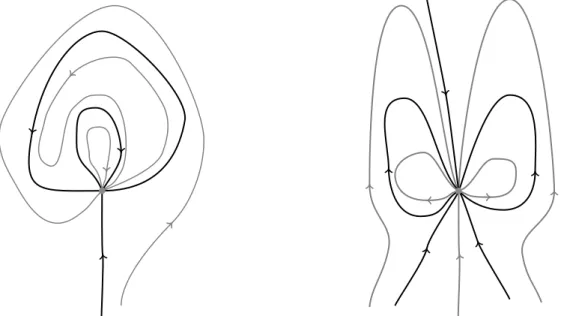
Figure 1.1: Two non-equivalent phase portraits with the same sectorial de- composition (elliptic-elliptic-hyperbolic-attracting-hyperbolic in counterclock- wise sense) at the origin.

labelling characterizes equivalence: topologically equivalent flows have the same canonical feasible set. We emphasize that although the separatrix skeleton is not uniquely defined, no ambiguity arises because the corresponding canonical feasible sets are the same (this follows from Lemma3.8).

Our first theorem summarizes these results.

Theorem A. Assume that0is a global attractor, non-positively stable, for two flowsΦandΦ⁰, both having finitely many separatrices, and let X and X⁰ denote their separatrix skeletons.

Then the following statements are equivalent.

(i) ΦandΦ⁰ are topologically equivalent.

(ii) X andX⁰ are compatible and the compatibility bijectionξ :X → X⁰ maps some hetero- clinic separatrix ofΦto a heteroclinic separatrix ofΦ⁰.

(iii) There are respective orientationsΘ,Θ⁰inR²and heteroclinic separatricesΣ,Σ⁰such that the associated canonical feasible sets are the same.

Contrary to what one might initially expect, the index of the global attractor plays no role in this topological classification. In fact, after extending the flow to the Riemann sphere, we get that ∞ is a repelling (topological) node (Remark 2.3). Hence, its index is 1 and, by the Poincaré–Hopf theorem [8, p. 179], the index of the attractor is 1 as well. Moreover, sharing (up to homeomorphisms) the same finite sectorial decomposition is a necessary but not suf- ficient condition for two such flows being topologically equivalent, see Figure1.1. Likewise, compatibility alone is not enough to guarantee topological equivalence, see Figure1.2.

Although the lemmas in Section3do not require finiteness of separatrices, no attempt has been done to find a more general version of TheoremAdisposing of this restriction. Anyway, we are mainly interested in polynomial (local) flows, that is, those associated to polynomial vector fields, hence finiteness of separatrices is guaranteed (Remarks 2.1 and2.4). Our next

2 3 4 5 7 6 9 8

10 11

12

13 14 15 16 17 18

19 20

21

22 23 24 25

26 27

28 1

2 3 4 5 7 6 9 8

10 11

12

13 14 15 16 17 18

19 20

21

22 23 24 25

26 27

28 1

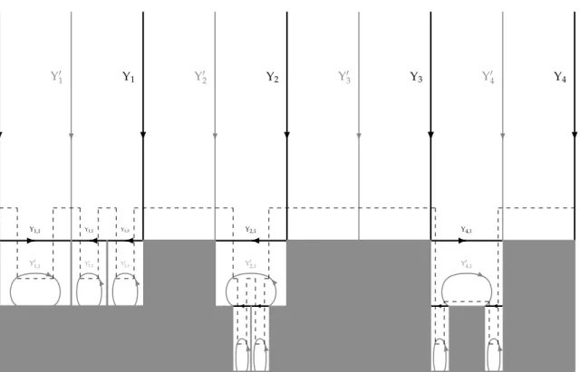
Figure 1.2: Two non-equivalent phase portraits with compatible separatrix skeleton (numbering indicating the compatibility bijection).

result, together with TheoremA, implies that if a flow has a globally attracting singular point, then it is equivalent to a polynomial flow.

Theorem B. Let L be a feasible set. Then there are a polynomial flow Φ (having 0 as a non-positively stable global attractor) and a heteroclinic separatrixΣ of Φ such that L is the canonical feasible set associated toΦ, the counterclockwise orientation inR²andΣ.

Our proof of TheoremBdepends heavily on the paper [19], where sufficient conditions are given allowing the associated flow to aC¹-vector field to be equivalent to a polynomial flow.

It is worth emphasizing that these conditions, as explained in that paper, are not necessary:

fortunately, the partial result in [19] turns out to be enough for our purposes. Still, this is not fully satisfying, because the arguments in [19] are essentially non-constructive. In fact, to the best of our knowledge, the literature provides no explicit examples of polynomial flows having a non-trivial globally attracting singular point. For this reason we finally prove:

Theorem C. The origin is both a global attractor and an elliptic saddle for the system (x⁰ =−((1+x²)y+x³)⁵,

y⁰ =y²(y²+x³). (1.1)

2 Preliminary notions

A number of standard topological notions will be of repeated use in this paper. We say that a topological space is an arc (respectively, open arc, circle, disk) if it is homeomorphic to [0, 1] (respectively, R, the unit circle S¹ = {(x,y) ∈ _R² : x²+y² = 1}, the unit disk {(x,y) ∈ _R² _: x²+y² ≤ ₁}_{). If} T is arc, and h : [_{0, 1}] → T is a homeomorphism, then h(₀) andh(1)are called theendpointsofT. Aregionof a topological spaceXis an open, connected subset ofX.

Alocal flowon a metric space(X,d)is a continuous mapΦ:Λ⊂_R×X→Xsatisfying:

• Λ is open inR×X; moreover, for any z ∈ X the set of numbers t for which Φ(t,z) is defined is an open interval Iz = (az,bz), with−_∞≤az <0<bz ≤_∞;

• Φ(0,z) =zfor any z∈ X;

• if Φ(t,z) =u, then I_u = {s−t : s ∈ I_z}; moreover, Φ(r,u) =_Φ(r,Φ(t,z)) =_Φ(r+t,z) for everyr ∈ I_u.

In the particular case Λ = _R×X, we call Φa flowon X. Observe that if X is compact, then Iz =_Rfor anyz ∈X, that is, any local flow onX is a flow. We writeΦz(t) =_Φt(z) =_Φ(t,z) whenever it makes sense, when observe that if Φ is a flow, then the map Φt : X → X is a homeomorphism for every t. We call ϕ_Φ(z) _:= _Φz(I_z). Here (as for the subsequent notions) we typically omit Φ in the subindex and write ϕ(z) instead. If ϕ(z) = {z} (when Iz = _R), then we callzasingular pointofΦ; otherwise the orbit, and its points, are calledregular. Since orbits foliate the space, that is, distinct orbits are disjoint, no point can be regular and singular at the same time. When the orbit ϕ(z) is a circle (equivalently, the map Φz(t) is periodic), it is called periodic. If I ⊂ I_z is an interval, then we call Φz(I) a semi-orbit of ϕ(z). In the particular cases I = [a,b] _{(with Φz}(a) = p, Φz(b) = q) I = [_0,b_z) _or I = (a_z, 0], we rewrite Φz(I)asϕ(p,q),ϕ(z,+)or ϕ(−,z), respectively. We define theω-limit setof the orbitϕ(z)(or the pointz) as the set

ω(z) ={u∈ X:∃tn→bz; Φz(tn)→u}. The α-limit setα(z)is analogously defined (nowt_n→ a_z).

We say that an orbitΓ ispositively(respectively, negatively) stableif for any p ∈ _Γ and any e>0 there is a numberδ > 0 (depending of pande) such that ifd(p,q)< δ, then all points from ϕ(q,+) (respectively, ϕ(−,q)) stay at a distance less than e from ϕ(p,+) (respectively, ϕ(−,p)). We say that Γ is stable if it is both positively and negatively stable, and we say that it is unstableif it is not stable. It is worth emphasizing that these notions are not purely topological: they depend on the metricd.

A setΩ ⊂ X is invariantfor Φ if it is the union of some orbits of Φ. If the restriction of Φto Λ∩(_R×_Ω) is a local flow on Ω (for instance, if Ωis invariant), then we call it, more simply if somewhat incorrectly, therestriction ofΦtoΩ.

Let Φ and Ψ be respective local flows on the spaces X and Y. We say that Φ and Ψ are topologically equivalentif there is a homeomorphismh:X →Ysuch thath(ϕ_Φ(z)) =ϕ_Ψ(h(z)) for every z∈X which preserves the respective (time) directions ofΦandΨ.

Local flows are associated, in a natural way, to (autonomous) systems of differential equa- tions defined on smooth manifolds M (which will be seen here as embedded inR^m for some natural number m). Namely, if Φ : Λ⊂ _R×M → M is a smooth local flow, then the vector field f :M →_R^m given by f(z) = ^∂Φ_∂t(0,z)(theassociated vector fieldtoΦ) is tangent to M and satisfies ^∂Φ_∂t(t,z) = f(_Φ(t,z)), that is, the solution of the systemu⁰ = f(u)with initial condi- tion u(0) = z is the map Φz(t) := _Φ(t,z), t ∈ Iz. Conversely, if a vector field f : M → _R^m is tangent to M and sufficiently smooth (locally Lipschitz is enough), and Φz(t)denotes the solution of u⁰ = f(u)_satisfying u(₀) = z, then Φ(t,z) _:= _Φz(t)is a local flow on M. While polynomial vector fields are the primary interest of this paper, and their associated flows are usually just local, there is a way to get rid of this restriction. In fact, if X is locally compact, O ⊂ Xis open, and Φ is a local flow onO, then there is a flow Ψ on X whose restriction to Ohas the same orbits and directions as those ofΦ, and having singular points outsideO[13, Lemma 2.3]. To simplify the notation we will callΦ, rather thanΨ, this extended flow, hoping that this will not lead to confusion. If Φ is associated to a polynomial vector field, then we

also call it (and its extension)polynomial, although of course this map is not “polynomial” in the usual sense.

In concrete, we are interested in the caseO=_R² andX=_R²_∞= _R²∪ {_∞}(the one-point compactification of R²), when after identifying R²_∞ with the Euclidean unit sphere S² ⊂ _R³ via the stereographic projection (u,v,w) 7→ (x,y) given by x = u/(1−w), y = v/(1−w), we use inR²_∞(and then inR²) the distanced(·,·)inherited from the Euclidean distance inS². Hence, the topologies onR² andR²_∞ are the usual ones but d(z,z⁰) ≤ 2 for any z,z⁰ ∈ _R²_∞. Unless otherwise stated, topological properties of subsets of R² refer to the topology in R². In particular, we mean A ⊂ _R² _{to be} bounded in the conventional sense, that is, when it is contained in an Euclidean plane ball (while, of course, all sets inR²are “bounded” regarding the distanced(·,·)).

Sphere and plane local flows have, as it is well known, some particularly good dynamical properties. The reader is assumed to be familiar with the basic facts of the Poincaré-Bendixson theory; for instance, recall that ifzis regular, then there is a transversal tozfor this flow. (If a local flowΦcan be restricted to a neighbourhoodAofzso that it is topologically equivalent to that induced by the constant vector fieldf₀= (1, 0)on the squareS= (−1, 1)×[−1, 1], and the arcT ⊂ Ais the image of the vertical arc{0} ×[−1, 1]by the corresponding homeomorphism h:S→ A, withh(0) =h(0, 0) =z, thenTis called atransversaltozforΦ, or just a transversal toΦ—or simply a transversal— when no emphasis onzis required. If all subarcs of an open arc or a circleQare transversal to Φ, we similarly say thatQistransversalto Φ.)

There is a natural way to transport polynomial vector fields from S² to R². Namely, if f : S² → _R³ is a polynomial vector field, tangent to S² and vanishing at the north pole (0, 0, 1)of S², say f(u,v,w) = (P(u,v,w),Q(u,v,w),R(u,v,w)), then we can carry it, via the stereographic projection, to the plane vector field

g(x,y) = (1−w)⁻¹(P(u,v,w) +R(u,v,w)x,Q(u,v,w) +R(u,v,w)y)

with u = 2x/(1+x²+y²), v = 2y/(1+x²+y²), w = (x²+y²−1)/(1+x²+y²), and after multiplyinggby a appropriate power of 1+x²+y²we obtain a polynomial vector field whose associated (polynomial) flow is topologically equivalent to the flow induced by f on S²\ {(0, 0, 1)}.

2.1 On special flows and regions

The standing assumption in this paper is that0 is a globally attracting singular point for the flows Φ on R² we deal with, that is, ω(z) = {0}for any z ∈ _R². This is closely related to the notions of heteroclinicity and homoclinicity. We say that an orbit ϕ(z)of Φishomoclinic (respectively,heteroclinic) if (besidesω(z) ={0}) we have α(z) ={0}(respectively,α(z) =_∅

—that is,α(z) ={_∞}when using the extended flow toR²_∞). Of course, the singular point0is trivially homoclinic. IfΓis homoclinic, then we denote byE(_Γ)the disk enclosed by the circle Γ∪ {0}(or just the singleton{0}in the caseΓ= {0}). Since 0as a global attractor, any orbit ofΦis either heteroclinic or homoclinic (Lemma3.1).

Let f_i : R² → _R², 1 ≤ i ≤ 4, be the vector fields f₁(x,y) = (x,−y), f₂(x,y) = (−x,−y), f₃(x,y) = (x,y)_, f₄(x,y) = (x²−2xy,xy−y²)respectively. Also, let

A₁= {(x,y)∈_R²: 0≤ x,y<1,xy<1/2}, A₂= A₃= A₄ ={(x,y)∈_R² _{: 0}≤ x,y< _1,x²+y²<₁}_.

Figure 2.1: From left to right: a hyperbolic, an attracting, a repelling and an elliptic sector.

We remark that although the sets A_i are not open, f_i still induces a local flow Φi on A_i, 1 ≤ i ≤ 4. See Figure 2.1. Assume now that B is a set containing 0 and Φ induces a local flow on B which is topologically equivalent to Φi. Then we say that B is a hyperbolic, attracting, repelling or elliptic sector of Φ (at 0) when, respectively, i = 1, 2, 3, 4. The flow Φ is said to have the finite sectorial decomposition property (at 0) if either 0 is positively stable or has a neighbourhood which is the (minimal) union of at least two, but finitely many, hyperbolic, attracting, repelling and elliptic sectors (since Φ admits no periodic orbits, see also Proposition 3.9, this amounts to the standard definition to be found, for instance, in [8, p. 18]).

Remark 2.1. The typical case for this to happen is thatΦ is associated to a vector field (real) analytic at 0, see for instance [8, Chapter 3].

We call a region Ω ⊂ _R² radial (respectively, a strip) if it is invariant for Φ, and, when restricted to Ω, Φ is topologically equivalent to the flow induced by f2 on R²\ {0} (respec- tively, in the upper half-plane H = _R×(0,∞)). Needless to say, to define strips, one can equivalently use (as it is usually done) the associated flow to the constant vector field f₀ on R². If all orbits of a strip Ωare heteroclinic (respectively, homoclinic), then we callΩhetero- clinic (respectively, homoclinic) as well. Observe that, in general, the interior of a hyperbolic, attracting or repelling sector is not a strip because it is not invariant (it does not consist of full orbits of Φ). We say that the stripΩ isstrong if there are orbits Γ1,Γ2 in BdΩ such that the restriction ofΦtoΩ∪_Γ1∪_Γ2is equivalent to that of the flow induced by f₂on ClH\ {0}. If, moreover, ClΩ=_Ω∪_Γ1∪_Γ2∪ {0}, then we say thatΩissolid.

Remark 2.2. If Ωis a solid strip, then either all Ω, Γ1 and Γ2 are heteroclinic, or all of them are homoclinic. Otherwise, as it is easy to check, either (a) one of orbits, sayΓ1, is heteroclinic, Γ2 is homoclinic and Ω = _R²\(_Γ1∪E(_Γ2)), or (b) both Γ1 and Γ2 are homoclinic, with E(_Γ1)∩E(_Γ2) = {0}, and Ω = _R²\(E(_Γ1)∪E(_Γ2)). Use Lemma 3.2 to find a heteroclinic orbitΓ⊂Ω. Clearly,Γcannot disconnectΩ∪_Γ1∪_Γ2, which contradicts that Ωis strong.

IfQis a transversal circle (respectively, open arc) with the property that, for everyz ∈ Q, ϕ(z)intersects Qexactly atz, thenΩ=^S_z∈Qϕ(z)is radial (respectively, a strip). To construct the corresponding homeomorphism h : R²\ {₀} → _Ω (respectively, h : H → Ω) just fix a homeomorphism f :S¹→ Q(respectively, f :S¹∩_H→ Q) and writeh(e^−t+iθ) =_Φ(t,f(e^iθ)). Conversely, if Ω ⊂ _R² is radial (respectively, a strip) then there is a circle (respectively, an open arc) Q⊂ Ω, transversal to Φ, having exactly one common point with every orbit inΩ.

We call any such set Q a complete transversal to Ω. If Ω is a strong strip, then more is true:

there is a transversal arc Thaving exactly one common point with every orbit inΩand every orbitΓ1,Γ2. We callT astrong transversaltoΩ.

Remark 2.3. IfΩis radial, and the circleCis a complete transversal toΩ, then it must enclose 0. Hence all heteroclinic orbits intersectC, that is,Ωis the union set of all heteroclinic orbits of Φ; in other words, Φ admits one radial region at most (later we will see, Proposition3.9, that such a region does exist). Moreover, the circlesΦt(C)tend uniformly to ∞as t → −_∞.

In fact, if Dt ⊂ _R²_∞ is the disk containing ∞ and having Φt(C) as its boundary, then Dt = {_Φs(u) : u ∈ C,s ≤ t} ∪ {_∞}. Since these disks intersect exactly at∞, we get diam(D_t)→ 0 ast → −∞, and the uniform convergence to∞follows. As a corollary, all heteroclinic orbits are negatively stable.

Similarly, ifΩis a solid strip andTis a strong transversal toΩ, thenΦt(T)tends uniformly to 0 as t → _∞, and tend uniformly to 0 as t → −_∞in the homoclinic case, and to ∞ in the heteroclinic case. In particular, all orbits of a solid strip are stable, and if it is heteroclinic (respectively, homoclinic), then the flow induced by f₂on ClH(respectively, byf₄on the union set of 0 and all orbits intersecting the diagonal arc {(x,x) : 1/2 ≤ x ≤ 1}) is topologically equivalent to the restriction ofΦto ClΩ.

If an orbit is not contained in any solid strip, then it is called aseparatrix of Φ. Note that the union set X of all separatrices of Φ is closed. The components of R²\X are called the canonical regionsof Φ. A family of orbits ofΦconsisting of all its separatrices and exactly one orbit from every canonical region is called aseparatrix skeletonofΦ. Observe that any regular separatrix can belong to the boundary of, at most, two different canonical regions. Therefore, if the number of separatrices is finite, so it the number of canonical regions.

Remark 2.4. As indicated in Remark 2.3, any unstable orbit must be a separatrix. If Φ has the finite sectorial decomposition property, then Γ is a separatrix if and only if it is either the singular point, or includes a semi-orbit limiting a hyperbolic sector. In particular, Φhas finitely many separatrices andΓis a separatrix if and only if it is unstable.

The next result is a particular case of [15, Theorems 5.2 and 7.1], see also [16] and [9].

Proposition 2.5. Any canonical region ofΦis either radial or a strip.

Remark 2.6. A strip (even a strong strip) needs not be either heteroclinic or homoclinic. Nev- ertheless, if a canonical region is a strip, then it must be either heteroclinic or homoclinic (because, in this case, the set of its heteroclinic orbits and the set of its homoclinic orbits are both open; hence, by connectedness, one of them must be empty).

Theorem 2.7. Assume that 0 is a global attractor for two flows ΦandΦ⁰ and let X andX⁰ denote some separatrix skeletons for Φ and Φ⁰. Then Φ and Φ⁰ are topologically equivalent if and only if there is a homeomorphism from the plane onto itself mapping the orbits ofX onto the orbits ofX⁰ and preserving the flows directions.

Remark 2.8. Our definition of separatrix is not the standard one (compare to [15], [16], [17, p. 294] or [8, p. 34]), even when we restrict ourselves, as it is the case here (Lemma 3.1), to flows having only heteroclinic or homoclinic orbits. More precisely, our “separatrices” are what we called “separators” in [9] (and our “canonical regions” what we called “standard regions” there). If the boundary of a heteroclinic strip consists of the singular point and two heteroclinic orbits, then it is solid (the corresponding strong transversal can be found with the help of Lemma3.7). If we replace “heteroclinic” by “homoclinic”, this needs not happen unless we additionally assume that the ordering “≺” we introduce below Lemma 3.2 totally orders the orbits of the closure of the strip. This point is missed in the above-mentioned references and, as a consequence, Theorem2.7, as stated there, does not work, see [9] for the details. Surprisingly, it seems that this fact has passed unnoticed until now.

2.2 On orientations and the extension of homeomorphisms

LetCbe a circle around0. IfΓis heteroclinic, we call the last point ofΓinC(that is, the point q∈ _Γ∩C such thatΦq(t) ∈/ C for any t > 0) the ω-pointof Γin C. Likewise, if Γ is regular and homoclinic and C is small enough so that there are points of Γ not enclosed by C, then we call the first and last points ofΓ in C(that is, the points p,q∈ _Γ∩Csuch that Φp(t)∈/ C for any t<0 andΦq(t)∈/Cfor any t>0) theα-pointand theω-pointof ΓinC, respectively.

If P is a finite family of orbits of Φ, and C is a circle around 0 small enough, then we denote by ∆_Φ(P,C) the set of all α- and ω-points in C from the orbits in P and call it the configuration of P in C. Note that the possibility that the singular point belongs to P is not excluded, when of course it adds no points to∆_Φ(P,C). Also, observe that all configurations of P are essentially the same, that is, if C and C⁰ are small circles around 0, then there is an orientation preserving homeomorphism h : C → C⁰ mapping the α- andω-points in Cof every orbitΓ∈ P to theα- andω-points inC⁰ of that same orbitΓ.

We call a triplet(A,B,C)of arcs inR²_∞sharing a common endpoint p(and no other point) a triod. The point p is called the vertex of the triod, the other endpoints of the arcs A,B,C being called itsendpoints.We say that the triod(A,B,C)ispositive, when, after taking an open euclidean ball U of center p and radius e > 0 small enough, there is θ₀ ∈ _R such that the first intersection points of these arcs with BdUcan be written as p+ee^iθA,p+ee^iθB,p+ee^iθC, with θ₀ = θ_A < θ_B < θ_C < θ₀+2π. We say that the triod isnegative when it is not positive.

Observe that the definition above excludes the case when the common endpoint p is∞. We then say that (_A,B,C)is positive when(_G(_A)_,G(_B)_,G(_C))is negative, G : R²_∞ → _R²_∞ being defined by G(z) = 1/z (here we identify R² with C and mean G(_∞) = 0, G(0) = _{∞). If}C is a circle around 0and (q,q⁰,q⁰⁰)is a triplet of distinct points in C, then we call itpositiveor negative according to whether it is counterclockwise or clockwise oriented inC, that is, there is a positive (negative) triod(A,A⁰,A⁰⁰)in the disk enclosed byCwith vertex0and endpoints q,q⁰,q⁰⁰. If Γ is homoclinic, then we say that it is positive (respectively, negative) when, after takingΓ⁰ ⊂IntE(_Γ)and a small circleCaround0, theα- and ω-points p,qof ΓinC, and the ω-pointq⁰ofΓ⁰inC, we get that(p,q⁰,q)is positive (respectively, negative). In simpler words, Γis positive (negative) when the flow induces the counterclockwise (clockwise) orientation on Γ∪ {0}.

Let P,P⁰ ⊂ _R² (respectively, P,P⁰ ⊂ _R²_∞). We say that Pand P⁰ areR²-compatible (respec- tively, R²_∞-compatible) if there is a homeomorphism H from R² (respectively, R²_∞) onto itself mappingPontoP⁰. Clearly,R²-homeomorphisms amount toR²_∞-homeomorphisms mapping

∞to itself. IfH :R²_∞ →_R²_∞is a homeomorphism, then, as it is well known, either it preserves the orientation, that is, all pairs of triods (A,B,C) _and (H(A)_,H(B)_,H(C)) have the same sign, or it reverses the orientation, that is, all pairs of triods(A,B,C)and(H(A),H(B),H(C)) have opposite sign. As it turns out, see [1], this is the key property to identify compatibility:

two Peano sets P and P⁰ (by aPeano space we mean a compact, connected, locally connected set) in R²_∞ are R²_∞-compatible if and only if there is a homeomorphism h : P → P⁰ either preserving or reversing the orientation, in the former sense, for all pair of triods (A,B,C) and(h(A),h(B),h(C))in PandP⁰ (whenhcan indeed be homeomorphically extended to the wholeR²_∞).

The former result can be adapted to theR²-setting as follows. We say that P⊂ _R² _isnice if it is unbounded, P_∞ = P∪ {_∞} is a Peano subset ofR²_∞, and for any triod (A,B,C) in P_∞ with vertex ∞there is a θ-curve in P_∞ including A, B and C (by aθ-curve we mean a union of three arcs intersecting exactly at their endpoints). Then we get: two nice sets P,P⁰ areR²-

compatible if and only if there is a homeomorphismh :P→P⁰either preserving or reversing the orientation for all pair of triods(A,B,C)and(h(A),h(B),h(C))inPandP⁰ (when, again, hcan indeed be homeomorphically extended to the wholeR²).

Assume that P and P⁰ are finite families of orbits of, respectively, Φ and Φ⁰ (we also assume that both of them contain the globally attracting singular point 0 and at least one heteroclinic and one homoclinic orbit). Let P and P⁰ be the union sets of these orbits and note that these sets are nice. Then, as it is simple to check, a condition characterizing the R²-compatibility of P and P⁰ (when we accordingly say that P and P⁰ are compatible) is the existence of acompatibility bijection. By this we mean a bijection ξ :P → P⁰ for which there is a homeomorphismµ:C→C⁰, withCandC⁰ small circles around0, mapping ∆_Φ(P,C)onto

∆_Φ⁰(P⁰,C⁰), so that µ(C∩_Γ) = C⁰∩ξ(_Γ) for any Γ ∈ P. In this case we say that µpreserves orbits forξ.

If, additionally,µmaps ω-points onto ω-points (when we say thatµpreserves directions for ξ), then the corresponding plane homeomorphism preserves the flows directions on P and P⁰. If, moreover, these families are the separatrix skeletons ofΦandΦ⁰, Theorem2.7 implies that the flows are equivalent.

2.3 A lemma on Janiszewski spaces

A compact connected Hausdorff space is called acontinuum. We say that a topological space Xis aJaniszewski spaceit is a locally connected continuum and, moreover, for any subcontinua C₁,C₂⊂ Xwith the property thatC₁∩C₂is not connected, there are pointsx,y∈ X\(C₁∪C₂) which are simultaneously contained in no subcontinuum inX\(C₁∪C₂). By [14, Fundamen- tal Theorem 6, p. 531], a topological space X is homeomorphic to R²_∞ if and only if it is a Janiszewski space, contains more than one point, and, for any x ∈ X, the set X\ {x} is con- nected. If Xis a Janiszewski space,Y is Hausdorff and there is a continuous monotone map mappingXontoY, thenYis Janiszewski as well (we say that f :X→Yismonotoneif f⁻¹(A) is connected wheneverA ⊂Y is connected). In fact, this is proved in [14, Theorem 9, p. 507]

additionally assuming thatYis a locally connected continuum; but ifXis a locally connected continuum,Y is Hausdorff, and X can be continuously mapped onto Y, then Y is indeed a locally connected continuum, as seen in [14, Theorem 9, p. 259].

Let K ⊂ _R²_∞ be a continuum such that R²_∞\K is connected. We define the equivalence relation “∼_K” inR²_∞byx ∼_K yif eitherx= yor bothxandybelong toK. Then we have:

Lemma 2.9. The quotient spaceQ=_R²_∞/∼_K is homeomorphic toR²_∞.

Proof. According to the previous discussion, ifΠ:R²_∞ → Qis the projection map (when recall that U is open in Q if and only if Π⁻¹(U)is open in R²_∞), then, in order to prove that Q is homeomorphic toR²_∞, we just need to show:

(i) Qis Hausdorff;

(ii) Q \ {X}is connected for anyX∈ Q;

(iii) Π⁻¹(C)is connected for any connected set C ⊂ Q.

Statements (i) and (ii) are immediate because of the assumptions onK. To prove (iii) we use that Π is a closed map by (i) and then apply [14, Theorem 9, p. 131] and the fact that any X∈ Qis a connected subset ofR²_∞.

3 General results on global attraction

Recall that we assume that0is a global attractor forΦ.

Lemma 3.1. All orbits ofΦare either homoclinic or heteroclinic.

Proof. If the statement of the lemma is not true, then there is some point z ∈ _R² such that α(z) contains a regular point u. Let T be a transversal to u. According to some well-known Poincaré–Bendixson theory, we can find p,q ∈ ϕ(z)∩T so that ϕ(p,q)∪S (where S is the arc in T whose endpoints are p and q) is a circle enclosing a disk D in R²_∞ which contains ϕ(−_,p), and henceα(z), and intersectsϕ(q,+) _{just at}q. This is impossible: on the one hand, 0cannot belong to D, because it is theω-limit set ofϕ(q); on the other hand,u∈α(z)implies ω(u)⊂α(z), so0does belong toD.

Lemma 3.2. The union set of all homoclinic orbits ofΦis bounded.

Proof. Assume the opposite to find a family of homoclinic orbits {ϕ(zn)}^∞_n=1 with zn → _∞ as n → _∞ and fix a circle C around0. Using the continuity of the (extended) flow Φ at∞, there is no loss of generality in assuming that the semi-orbitsΦzn([−n, 0])do not intersect the regionOencircled by C. Next, find the numbersan ≤ −n, closest to −n, such that the points Φzn(a_n)belong to C (using that the orbits ϕ(z_n) are homoclinic) and assume, again without loss of generality, that the points u_n = _Φzn(a_n)converge to u. SinceΦun(t) ∈ _R²\O for any t ∈ [0,n], the continuity of the flow implies that ϕ(u,+) does not intersect O, contradicting that 0is a global attractor.

Let H denote the family of homoclinic orbits of Φ. We introduce a partial order in H by writing Γ _Σ if Γ ⊂ E(_Σ), when Γ ≺ _Σ means of courseΓ _Σ with Γ 6= Σ. We say that Γ ∈ H _is maximal if there is no Σ ∈ H _{such that Γ} ≺ _{Σ. If Γ,Σ} ∈ H and neither Γ _{Σ nor} Σ _Γ is true, then we say that Γ and Σ are incomparable. Realize that a family of pairwise incomparable orbits must be countable. Moreover, we have the following lemma.

Lemma 3.3. If the orbits{_Γn}^∞_n=1are pairwise incomparable, thendiam(_Γn)→0as n →_∞.

Proof. Suppose the contrary to get a pointu 6= 0 at which these orbits accumulate. Let T be a transversal to u and find points u_nk ∈ _Γnk∩T, k = 1, 2, 3, with, say, u_n2 lying between u_n1 and un₃ in T. Then un₁ andun₃ belong to different regions inR²\(_Γn2∪ {0}): we are using here that any homoclinic orbit can intersect a transversal at one point at most. Thus, either Γn1 ≺ _{Γn2 orΓn3} ≺_Γn2, contradicting the hypothesis.

Lemma 3.4. LetΩ$R²be a region invariant forΦ.

(i) IfΩis bounded, thenBdΩis the union set of a homoclinic orbitΣ, a (possibly empty) familyG of pairwise incomparable homoclinic orbits satisfying Γ ≺ _Σfor every Γ ∈ G, and the singular point.

(ii) IfΩis unbounded, then its boundary is the union set of at most two heteroclinic orbits, a (possibly empty) family of pairwise incomparable homoclinic orbits, and the singular point.

Proof. SinceΩin invariant, BdΩis invariant as well, and the statement (ii) follows easily from the connectedness of Ω. To prove (i), assume that the boundary of the bounded region Ωis not as described and realize that then we must have BdΩ = {0} ∪^S_nΓn for a family {_Γn}_n (having at least two elements) of pairwise incomparable homoclinic orbits. Lemma3.3implies

thatO=_R²\^S_nE(_Γn)is a region including Ωwith the same boundary asΩ. HenceΩ=O, contradicting thatΩis bounded.

Lemma 3.5. LetΓ∈ H. Then there isΣ∈ H, maximal for “≺”, such thatΓ_Σ.

Proof. If Γ is not maximal itself, then the Jordan curve theorem implies that the non-empty familyF = {_Γ⁰ ∈ H : Γ _Γ⁰} is a totally ordered subset ofH; accordingly, it is enough to show thatF has a maximal element for_.

Say F = {_Γi}_i. Then, because of the total ordering, Ω= ^S_iIntE(_Γi)is a region invariant for Φ, and because of Lemma 3.2, Ω is bounded. As a result, we can apply Lemma 3.4(i) to obtain the corresponding homoclinic boundary orbit Σ. Then, clearly, Σ is the maximal element ofF.

Remark 3.6. Note that all maximal homoclinic orbits ofΦare separatrices.

Lemma 3.7. Let z be a regular point. Then there is a transversal T to z such that, for every u ∈ T, ϕ(u)intersects T exactly at u.

Proof. Fix an arc Qtransversal toz. Note that no orbit can intersectQinfinitely many times.

Also, if some orbit intersectsQat consecutive times t <s and corresponding pointsuandv, then no orbit can intersect the open arc inQwith endpoints u andv more than once. Using these two facts it is easy to construct a transversalT ⊂Qtozwith endpointspandqsuch that the orbits ϕ(p)and ϕ(q)intersect Tat exactly pandq. This is the transversal we are looking for, because if an orbitΓconsecutively intersectsT at pointsuandv, andDis the disk inR²_∞ enclosed by ϕ(u,v)and the arc inT with endpointsuandvsuch that0∈D, then either ϕ(p) or ϕ(q)does not intersect D, a contradiction.

Lemma 3.8. If Ωis a canonical region and Γ,Γ⁰ are distinct orbits in Ω, then there is a solid strip S⊂_Ωsuch thatBdS=_Γ∪_Γ⁰∪ {₀}.

Proof. LetQbe a complete transversal toΩand letA⊂ Qbe an arc with endpoints belonging to Γ and Γ⁰. Since Ω includes no separatrices, for any point z ∈ Q there is a solid strip in Ω, containing z, whose closure intersects Q at a small arc in Q (this small arc thus being a strong transversal to the strip). Taking this into account, and applying a simple compactness argument toA, the lemma follows.

Recall that Φadmits one radial region at most, that consisting of all heteroclinic orbits of Φ(Remark2.3). Indeed, such is the case:

Proposition 3.9. Let R be the union set of all heteroclinic orbits ofΦ. Then it is radial. Moreover:

(i) If R=_R²\ {0}, that is, all regular orbits ofΦare heteroclinic, thenΦis topologically equivalent to the associated flow to f2(x,y) = (−x,−y) inR² (hence 0 is positively stable and it is the only separatrix ofΦ).

(ii) If R6=_R²\ {0}, then R includes a separatrix ofΦ.

Proof. First we assume R = _R²\ {0}. To prove that R is radial and (i) holds, it suffices to show that 0 is the only separatrix of Φ (Proposition 2.5 and Theorem 2.7). Take z ∈ R and letT ⊂ Rbe an arc transversal toz with the property that the orbits of all its points intersect T exactly once (Lemma 3.7). Let p andq be the endpoints of T and let Dbe the disk in R²_∞ enclosed byϕ(p)_, ϕ(q)_,0and∞and includingT. Ifu∈_IntD, thenϕ(u)_intersectT(because

it is heteroclinic). Therefore, IntD is a heteroclinic solid strip; in particular, ϕ(z) is not a separatrix.

Assume now R 6= _R²\ {0}. Applying Lemma 2.9 to the union setK = _R²\R of all sets E(_Γ)withΓmaximal for “≺" (recall also Lemmas3.3and3.5), and using (i), we can construct a topological equivalence between the restriction ofΦtoRand the restriction (toR²\ {0}) of the associated flow to f₂. In particular,Ris radial.

To prove the last statement of the proposition, assume that R includes no separatrices (hence it is a canonical region by Proposition 2.5), fix a complete transversal circleCto Rand apply Lemma3.8(recall also Remark2.3) to conclude the uniform convergence ofΦt(C)to0 and∞ast→ ±_{∞. Then}R=^S_t∈RΦt(_C) =_R²\ {0}, a contradiction.

4 Proof of Theorem A

In this section we assume, besides global attraction, that 0is not positively stable and Φhas finitely many separatrices.

LetX be a separatrix skeleton forΦ, fix a small circle Caround 0and let X = _∆Φ(X_,C) be the configuration of Φin C. Also, fix an orientation Θ(counterclockwise or clockwise) in R² and a heteroclinic separatrix Σ in X (such an orbit exists because of Proposition3.9(ii)).

Letqbe theω-point ofΣinC. Find disjoint open arcs J,J⁰ ⊂Cwhose closures have qas their common endpoint (small enough so that they do not contain any points from X), take points p ∈ J, p⁰ ∈ J⁰, and assume that they are labelled so that the orientation of(p,q,p⁰)inCis that given by Θ (that is, (p,q,p⁰)is positive if and only if Θ is the counterclockwise orientation).

Finally, after removing J⁰ fromC, we get an arcAwith endpointsa(the other endpoint of the closure of J⁰) andq, and order the points from Ain the natural way so thata<q.

We call positive (negative) homoclinic orbitseven whenΘis the counterclockwise (clock- wise) orientation, and odd when Θ is the clockwise (counterclockwise) orientation. Thus, a homoclinic orbit fromX is even if and only if itsα-pointvand itsω-pointwsatisfyv<w. By convention, all heteroclinic orbits are even. We say that two orbits have thesame paritywhen both are even or both are odd.

According to Proposition2.5 and, again, Proposition 3.9(ii), all canonical regions are in- deed strips, so we will call them canonical strips. Recall (Remark2.6) that any canonical strip must be either heteroclinic or homoclinic. By Lemma 3.4, the boundary of any heteroclinic canonical strip Ω consists of (apart from 0) two heteroclinic separatrices (or just Σ, when Ω= R\_Σis the union set of all heteroclinic orbits exceptΣ) and several (possibly zero) max- imal homoclinic separatrices (Remark3.6), whenΩis calledelementaryif and only if this last set is empty. Likewise, the boundary of a homoclinic canonical stripΩconsists of, apart from 0, a homoclinic separatrix Γenclosing it and possibly some others, all of them less than Γin the≺-ordering, when we again callΩelementaryif this last family is empty. Note that is quite possible for a canonical strip to be elementary, but at least one heteroclinic canonical strip cannot be elementary (otherwiseΦwould have no homoclinic separatrices, and consequently all its regular orbits would be heteroclinic, contradicting Proposition3.9(i)).

Remark 4.1. The following statements are easy to prove:

• a heteroclinic canonical strip is elementary if and only if it is solid;

• a homoclininic canonical strip is elementary if and only if the restriction of Φ to its closure is topologically equivalent to the flow induced by the “elliptic vector field”

f₄(x,y) = (x²−2xy,xy−y²) on the union set A₄⁰ of all orbits intersecting the diago- nal arc{(x,x), 0≤x ≤1}.

Remark 4.2. If a regular homoclinic separatrix Γ is minimal, that is, E(_Γ) is an elementary homoclinic canonical strip, then there is an elliptic sector intersectingE(_Γ)(Remark4.1). Thus, due to Remark2.4, if0is not positively stable, and the finite sectorial decomposition property holds, then the decomposition must include both an elliptic and a hyperbolic sector.

There are two natural ways to associate an orbit from X to each canonical strip Ωof Φ. Firstly,γ⁰(_Ω)will denote the orbit fromX included inΩ. Next,γ(_Ω)will denote (whenΩis homoclinic) the separatrixΓ⊂BdΩenclosingΩ, and (whenΩis heteroclinic) the heteroclinic separatrixΓ⊂_{BdΩwhoseω-point}w(inC, and then inA) satisfiesv<w,vbeing theω-point of γ⁰(_Ω). Note that X consists of all orbits γ(_Ω),γ⁰(_Ω) together with 0. Also, observe that γ⁰(_Ω)decomposesΩinto two componentsΩl andΩu,Ωubeing the component ofΩ\γ⁰(_Ω) includingγ(_Ω)in its boundary (an ambiguity arises in the caseΩ= R\_{Σ, whereΩuconsists} of the orbits whoseω-points are greater than theω-point ofγ⁰(_Ω)).

Lemma 4.3. Let Ωbe a canonical strip and let Γ be a regular orbit in BdΩ. Then Γ has the same parity asγ⁰(_Ω)if and only if eitherΓ=γ(_Ω)orΓ∈BdΩl.

Proof. We present the proof under the hypothesis thatΩis a heteroclinic strip whose boundary includes two heteroclinic orbits, γ(_Ω)and γ⁰⁰(_Ω). The case when Ω is heteroclinic butΣ is the only heteroclinic separatrix ofΦ, and the homoclinic case, can be dealt with in analogous fashion. We will also assume that the fixed orientation Θ is counterclockwise so the even (respectively odd) homoclinic orbits coincide with the positive (respectively negative) ones.

If Ωis elementary, then there is nothing to prove: both Γ andγ⁰(_Ω) are heteroclinic and consequently even. Otherwise, letΓ1, . . . ,Γj be the maximal homoclinic orbits in BdΩ, where these orbits are labelled in such a way that if q₁, . . . ,q_j are the correspondingω-points, then q₁ < · · · < q_j (in A). The corresponding α-points will be denoted by p_k, 1 ≤ k ≤ j. Finally, let u, v and w be the ω-points of γ⁰⁰(_Ω), γ⁰(_Ω) and γ(_Ω), respectively (so u < v < w). We can assume without loss of generality that there are small subarcs ofC, neighbouring all these points, which are transversal to the flow.

Let 1≤ k ≤ j−1. We claim that it is not possible that Γk is negative andΓk+1 is positive.

Assume by contradiction q_k < p_k < p_k+1 < q_k+1. Find points p_k < b < b⁰ < p_k+1 in C, very close to p_k and p_k+1, respectively, so that T = {t ∈ C : p_k ≤ t ≤ b}, T⁰ = {t ∈ C : b⁰ ≤ t ≤ p_k+1} are transversal to the flow. Also, let Q = {t ∈ C : b ≤ t ≤ b⁰}. Since Γk is negative, backward semi-orbits starting from points fromT\ {p_k}enter the disk D enclosed byCand, since Γk+1is positive, then they escape from the disk throughQ. Accordingly, take a a decreasing sequence(b_n)^∞_n=1inT∩_Ωtending top_k and find maximal semi-orbitsϕ(a_n,b_n) fully included in D, when observe that the sequence (a_n)_n, besides lying in Q, is increasing.

Calla^∗ its limit. Clearly,a^∗ ∈ClΩ. Since the full forward orbit ϕ(a^∗,+)lies in D, andΓk and Γk+1are consecutive, we easily get that, in fact,a^∗ ∈_Ωand there is a solid heteroclinic strip S neighbouring a^∗. This is impossible because points b_nbelong to Sif nis large enough, hence Γk ⊂BdS.

Further, if Γk and Γk+1 have the same sign, then γ⁰(_Ω) cannot lie between them. In fact, assume, say, q_k < p_k < v < q_k+1 < p_k+1, take b, T and (b_n)_n as before but consider now Q = {t ∈ C : b ≤ t ≤ v}. Find similarly the points an and a^∗ in Qto obtain the analogous contradiction. We prove that ifΓ1 is positive, then γ⁰(_Ω) cannot lie between γ⁰⁰(_Ω) and Γ1, and ifΓj is negative, thenγ⁰(_Ω)cannot lie betweenΓj andγ(_Ω), in the same way.

As a conclusion, we get that either (a) all orbitsΓk are positive andγ⁰(_Ω)lies between Γj

and γ(_Ω), or (b) all orbitsΓk are negative and γ⁰(_Ω) lies betweenγ⁰⁰(_Ω)andΓ1, or (c) there is 1 ≤ m ≤ j−1 such that all orbits Γk with k ≤ m are positive, all orbits with k > m are negative, andγ⁰(_Ω)lies between Γm andΓm+1. This implies the lemma.

We say that a finite, non-empty set V of vectors of positive integers iscompletewhen, for any (i₁, . . . ,i_l) ∈ V, we have(i₁, . . . ,im)∈ V for every 1 ≤ m≤ l, and (i₁, . . . ,i_l−1,i) ∈ V for every 1 ≤ i ≤ i_l. Ifv ∈ V, then we denote byλ(v)the largest number j such that(v,j) ∈ V, λ(v) =0 meaning that there is nojsuch that(v,j)∈V. Likewise,λ(_∅)stands for the largest number t such that (t)∈ V. Of course we should writeλ_V instead ofλ (and similarlyρ_L,σ_L instead of ρ,σ below) to emphasize that this map depends on V, but hopefully this will not lead to confusion.

LetM={n/3 :n=0, 1, 2, . . .}.

Definition 4.4. We say that a setLof vectors of numbers fromMisfeasiblewithbasea complete set V if its elements have the structure (v,k), with v ∈ V and k ∈ M, and the following conditions hold:

(i) for each (i) ∈ V of length 1 there are exactly two elements in L: (i,λ(i) +1) and (i,s+_2/3)for some integer s=σ(i)_{, 0}≤ s≤λ(i)_;

(ii) for eachv∈ Vof length at least 2 there are exactly four elements inL:(v, 0),(v,λ(v) +1), and(v,r+1/3),(v,s+2/3)for some integersr =ρ(v),s= σ(v), 0≤r≤s ≤λ(v); (iii) (_i,λ(_i) +_2/3) _and (_i+_{1, 2/3}) cannot simultaneously belong to L (where we mean

i+1=1 wheni=λ(_∅));

(iv) if λ(v) =1, then (v, 1/3),(v, 5/3),(v, 1, 1/3)and(v, 1,λ(v, 1) +2/3)cannot simultane- ously belong toL.

Note that property (iii) above implies thatλ(i) ≥ 1 for somei, hence V contains at least one sequence of length 2. If V is the base of a feasible set L, then we assign a parity (even or odd) to each v∈ V as follows. All vectors of length 1 inV have parity even. If (i)∈ V, then we assign even or odd parity to(i,j)depending on whether j≤ σ(i)or not. Inductively, once the parity of v ∈ V is established, we assign to (v,j)the same parity as v, or the other one, depending on whetherρ(v)< j≤ σ(v)or not. Finally, if w= (v,h)∈ L, then we say that w is an α-vectorif eithervis even and h= 0 orh= ρ(v) +1/3, or vis odd and h= λ(v) +1 or h=σ(v) +2/3. Otherwise, we say thatwis aω-vector.

We next explain how to associate canonically a feasible set Lto Φ. To construct the base V we proceed inductively, biunivocally associating to each canonical strip Ω (and the ω- point of γ(_Ω)) a vector from V. First of all, order the heteroclinic canonical strips of Φ as Ω1, . . . ,Ωt, this meaning that the corresponding ω-points q_i of the orbits γ(_Ωi), 1 ≤ i ≤ t, satisfyq₁< . . .< q_t. Then the 1-length vectors from Vwill be those of the type(i), 1≤i≤t.

If, additionally, the strip Ωi is not elementary, andΩi,1, . . . ,Ωi,j are the homoclinic canonical strips Ωsuch that γ(_Ω) ⊂ BdΩi (again assuming q_i,1 < . . . < q_i,j for their correspondingω- points), then we add the 2-vectors(i,k)toV, 1≤k≤ j. In general, if a vectorvhas been added to V, with corresponding canonical strip Ωv, and Ωv is not elementary, then we consider as before the homoclinic canonical strips Ωsuch thatγ(_Ω)⊂BdΩv, call themΩv,1, . . . ,Ωv,j⁰ (so thatq_v,1 <. . .<q_v,j⁰ for the correspondingω-points), and add the vectors (v,k), 1≤k ≤j⁰, to V. Clearly, the setV so defined is complete.

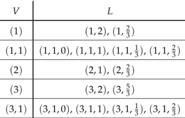
V L (1) (1, 2), (1,⁵₃)

(1, 1) (1, 1, 0),(1, 1, 2),(1, 1,¹₃),(1, 1,²₃) (1, 1, 1) (1, 1, 1, 0),(1, 1, 1, 1),(1, 1, 1,¹₃),(1, 1, 1,²₃)

Table 4.1: The elements of the feasible setLand its baseV from the left flow of Figure1.1.

V L

(1) (1, 2),(1,²₃)

(1, 1) (1, 1, 0),(1, 1, 1),(1, 1,¹₃),(1, 1,²₃) (2) (2, 1),(2,²₃)

(3) (3, 2),(3,⁵₃)

(3, 1) (3, 1, 0),(3, 1, 1),(3, 1,¹₃),(3, 1,²₃)

Table 4.2: The elements of the feasible set Land its baseV from the right flow of Figure1.1(Σis the “upper” heteroclinic separatrix).

Now we defineL(and biunivocally associate to its vectors all points fromX). We just must explain how to choose the numbers σ(i)and the pairs ρ(v),σ(v)in Definition4.4(i) and (ii), and then check that (iii) and (iv) hold. As for the first numbers, let (with the notation of the previous paragraph) 1 ≤ i ≤ t. Then s = σ(i) is the largest number such that q_i,s < y_i, y_i being the ω-point of γ⁰(_Ωi) (or s = 0 if Ωi is elementary or no such number exists, that is, y_i <q_i,j for all j). Also, we redefine the pointsy_i andq_i asc_i,σ(i)+_2/3 andc_i,λ(i)+₁, respectively.

In the general case we denote byx_v and y_v theα- and ω-points of γ⁰(_Ωv)when this orbit is even, reversing the notation whenγ⁰(_Ωv)is odd, and taker=ρ(v)ands=σ(v)as the largest numbers satisfyingqv,r < xv andqv,s <yv, respectively (orr = s =0 whenΩv is elementary, andr = 0 or s = 0 when the corresponding number does not exist). Finally, we redenote x_v andy_v as c_v,ρ(v)+1/3 and c_v,σ(v)+2/3, whilec_v,0 and c_v,λ(v)+1 stand for the α- and ω-points (or conversely in the odd case) ofγ(_Ωv).

We claim that (iii) in Definition4.4holds. Indeed if, say, both(i,λ(i) +2/3)and(i+1, 2/3) belong toL for somei, the orbitsγ⁰(_Ωi)_andγ⁰(_Ωi+1)would bound, together with0, a solid strip (Remark2.8). Since this strip includes the separatrix γ(_Ωi), we get a contradiction.

Assume now that Definition 4.4(iv) does not hold, that is, there is v ∈ V with λ(v) = 1 such that all vectors (v, 1/3), (v, 5/3), (v, 1, 1/3) and(v, 1,λ(v, 1) +2/3)belong to L. Then, again by Remark2.8, the orbitsγ⁰(_Ωv),γ⁰(_Ωv,1)bound, together with0, a solid strip including γ(_Ωv,1), which is impossible.

Thus we have shown that Lis feasible. Although Lhas been constructed with the help of the circleC, it depends only on Θ andΣ. We call it the canonical feasible set associated to Φ, the orientationΘand the separatrix Σ.

As some examples, we present in Tables4.1and4.2the feasible sets associated to the flows on Figure1.1under the counterclockwise orientation.