Az a priori ismeretek alkalmazása a vegyipari folyamatmérnökségben

(1)

DOKTORI (PhD) ÉRTEKEZÉS

Madár János

Veszprémi Egyetem

2005.

(2)

(3)

Veszprémi Egyetem Folyamatmérnöki Tanszék

A Z A PRIORI ISMERETEK ALKALMAZÁSA A VEGYIPARI FOLYAMATMÉRNÖKSÉGBEN

DOKTORI (PhD) ÉRTEKEZÉS

Madár János

Témavezető dr. Abonyi János

Veszprémi Egyetem Vegyészmérnöki tudományok Doktori Iskolája

2005

(4)

(5)

Az a priori ismeretek alkalmazása a vegyipari folyamatmérnökségben

Értekezés doktori (PhD) fokozat elnyerése érdekében

Írta:

Madár János

Készült a Veszprémi Egyetem Vegyészmérnöki Doktori Iskolája keretében

Témavezető: dr. Abonyi János

Elfogadásra javaslom igen / nem ……….

(aláírás) A jelölt a doktori szigorlaton …... %-ot ért el,

Az értekezést bírálóként elfogadásra javaslom:

Bíráló neve: …...…... igen / nem

……….

(aláírás)

Bíráló neve: …...…... igen / nem

……….

(aláírás)

A jelölt az értekezés nyilvános vitáján…...%-ot ért el

Veszprém, ……….

a Bíráló Bizottság elnöke

A doktori (PhD) oklevél minősítése…...

………

Az EDT elnöke

(6)

(7)

KIVONAT

Az a priori ismeretek alkalmazása a vegyipari folyamatmérnökségben

A doktori értekezés a vegyipari folyamatok, különös tekintettel a kémiai reaktorok, modellezéséhez, szabályozásához és optimalizálásához járul hozzá. A vegyipari folyamatok modellezése, modell alapú szabályozása és optimalizálása a folyamatmérnökség nagy jelentőséggel bíró, dinamikusan fejlődő ága. Ez a szerteágazó terület még ma is sok megoldatlan problémával szolgál, mivel a folyamatmérnöki problémák megoldása során a feladat konkrét jellegétől függően más és más módszerek állnak rendelkezésre, amelyek sok esetben nem hasznosítják az összes rendelkezésre álló ismertet. A doktori értekezésben a szerző olyan új számítási intelligencia eszközöket mutat be, amelyek alkalmasak a különféle formában rendelkezésre álló információk beépítésére a jellemző folyamatmérnöki problémák megoldásába, különös tekintettel az a priori információknak a mérési adatokon alapuló módszerekben történő felhasználására.

A kidolgozott módszerek négy tárgykört érintenek. Az első tárgykör a folyamatoptimalizálás. A folyamatoptimalizálásban gyakori probléma, hogy egymásnak ellentmondó, nehezen formalizálható vagy számszerűsíthető célokat kell egy időben figyelembe venni. A szerző egy olyan interaktív optimalizáló algoritmust dolgozott ki, amely a konfliktusokat és az egymásnak ellentmondó feltételeket úgy kezeli, hogy bevonja a folyamatmérnököt a megoldások értékelésébe. A módszer gyakorlati hasznosságát a szerző egy biokémiai reaktor és egy MPC szabályozó szimulációs optimalizálási példájával demonstrálja.

A második tárgykör a fekete doboz modellek struktúra identifikációja. A szerző egy olyan új módszert mutat be, amely struktúra identifikáció során kiszűri a felesleges tagokat a modellből, és ezáltal egyszerűbb, áttekinthetőbb modelleket kapunk. A kidolgozott algoritmus nemcsak dinamikus nemlineáris modell struktúrák identifikációjára, de modellrendűség meghatározására is használható. A szerző a módszer hatékonyságát kémiai reaktorok modellrendűségének vizsgálatával illusztrálja.

Az értekezés következő tárgyköre a mérési adatokon alapuló kinetikai paraméterbecslés. A kidolgozott módszer a szokásos módszerekhez hasonlóan a mérési adatpontokra függvényt illesztve becsüli a paramétereket. Miközben a hagyományos módszerek csak a mérésből rendelkezésre álló információt hasznosítják, addig a bemutatott módszer a rendelkezésre álló a priori ismereteket is hasznosítja, és ezáltal megbízhatóbb és elfogadhatóbb paraméterbecslést eredményez. A kifejlesztett módszert a szerző egy szimulált reaktor és egy ipari reaktor mérési adatainak felhasználásával szemlélteti.

Az értekezés utolsó tárgyköre a linearizáláson alapuló szabályozótervezés. A szerző egy olyan hibrid modellt mutat be, amely kombinálja az a priori modellezést és az a posteriori modellezést olyan módon, hogy egy mesterséges neurális hálózat helyettesíti a fehér doboz modell megismerési szempontból bizonytalan részét. Ennek a hibrid modellezési technikának az előnye a szokásos a priori modellezés technikával szemben az, hogy kevésbé érzékeny a paraméter bizonytalansággal szemben, amit a szerző egy kevert üstreaktor input-output linearizálásos szimulációs szabályozási példáján keresztül mutat be.

(8)

ABSTRACT

The application of a priori knowledge in chemical process engineering

Because the lack of knowledge and understanding of complex and nonlinear processes in chemical engineering and the fact that information comes from a vast range of different sources, the incorporation of different types of knowledge into the solution of chemical process engineering problems is a challenging and important task, which motivated the research presented in this doctoral dissertation. The author points out that simultaneous usage all available information sources are very important. The dissertation proposes new methods for the optimization and identification of models, controllers and processes with the combination of several type of information. The author demonstrates with several examples that the proposed methods lead to more efficient and reliable solutions than standard methods.

РЕЗЮМЕ

Применение приоритетных информаций в химических технологических процессах

Поскольку комплексные и нелинеарные процессы в химической технологии не полностью известны и поскольку имеется много информаций из источников широкого спектра, поэтому применение этих информаций в решении проблем химических процессов является очень важной и трудной задачей, и это послужило мотивацией темы этой докторской диссертации.

Автор диссертации указывает на то, что очень важно одновременное использование всех информационных источников. Докторская диссертация предлагает новые методы по оптимализации моделей, регуляторов и процессов, которые комбинируют различные типы информациий. Автор на многих примерах демонстрирует, что предлагаемые им методы намного эффективнее и надёжнее, чем стандартные методы.

(9)

Acknowledgement

The work resulted in the dissertation has been aided and supported by many people and the author is greatly indebted to all.

First of all, I wish to thank my parents not only for their continuous support but because I have inherited the love of science from them. I am grateful tomy brother and sister because I have inherited more personal traits than I ever realized.

I am very grateful to theProcess Engineering Department at the University of Veszpr´em, where I have studied and worked during the past years, for the helpful and inspirative atmosphere and the friendly working environment.

I am very indebted to my supervisorsProf. Ferenc Szeifert andDr. J´anos Abonyi for their excellent guidance and endless support during my work and study. I especially wish to thank Dr. J´anos Abonyi, without his great support this thesis would probably not have come into existence.

I am very grateful toDr. G´abor Szederk´enyi from Computer and Automa- tion Research Institute of the Hungarian Academy of Sciences and to Dr.

J´ozsef Tar from Budapest Polytechnic for their useful advices and remarks.

Some part of this thesis are based on a paper co-authored by Dr. Hans Roubous from Delft University of Technology. This work has also benefited from the help of Dr. Tibor Chován and Dr. Lajos Nagy from Department of Process Engineering andGábor Madár from Department of Image Processing and Neurocomputing, I would like to thank them their co-operation.

I am indebted also to Zsuzsanna B´eres, Aba Boros and Dr. T¨unde Stribl, they always helped me to solve all of the administrative and technical problems.

I would like to acknowledge the support of Cooperative Research Center (VIKKK) (Project 2001-I-7).

(12)

(13)

1 Introduction

1.1 The Scope of the Thesis

The motivation of this doctoral dissertation is to present new approaches for chemical process engineering, especially in the area of modeling, control and optimization of chemical reactors.

Modeling, control and optimization of chemical reactors very often lead to optimization tasks. For example, modeling of a system requires optimization of model parameters, application of a controller needs to tune the parameters.

Since most chemical processes have complex nonlinear behavior, it is often necessary to solve complex and diﬃcult nonlinear optimization problems in chemical process engineering. In order to solve this kind of optimization problems, it is worth employing every available knowledge related to the problem.

Fig. 1.1. Schematic concept of the Thesis

(14)

Figure 1.1 illustrates that information for process engineering problems can be obtained from diﬀerent sources:

• Measurement data. For example, input-output data from experiments.

• Mechanistic knowledge. For example,a priori information about the modeled process, the laws of physics and chemistry.

• Expert knowledge. For example, experience of the operating engineer.

In addition, there are some requirements which must be met:

• Accuracy. For example, a model must provide accurate predictions; a controller must control the system accurately (ﬁrst of all without steady-state error); the quality of a product must meet certain requirements.

• Interpretability. From the aspect of practical usefulness, it is important that the result be simple, interpretable. For example, if one would like to use the resulted model to design a model-based controller then the design of controller will be more eﬀective if it is based on a transparent model.

Eﬀective problem solving requires the usage of every available information sources. The usage of diﬀerent types of knowledge is a challenging and important task. This complex task motivated the research presented in this thesis.

Therefore the subject of the thesis is not only solving some speciﬁc problems but analyzing and developing new approaches for typical chemical engineering problems, especially in consideration of chemical reactors. For example, the combination of expert knowledge with computational techniques was the subject of Chapter 2, the combination ofa priori knowledge with data driving techniques was the subject of Chapter 4. Each of the subsequent four chapters (Chapter 2-5) is devoted to a speciﬁc problem. These chapters are relatively independent from each other so each of them contains short introduction and summary. The following sections will provide general introduction and literature overview for the whole thesis.

1.2 Interactive Optimization for Process Control and Design

System identification, process optimization and controller design are often for- mulated as optimization problems. The key element of the formalization of optimization problems is defining the cost function. Cost function is a mathematical function that represents the objectives of the expected solution, and the goal is usually to find the minima (or the maxima) of this function. For example, the cost function of the well-known traveling salesman problem is the distance that the salesman travel by visiting given number of towns. In practice, there may be several objectives that should be taken into account when a cost function is defined, and these objectives may be in conflict with each other. Under these circumstances, the cost function must reflect the rel- ative importance of the conflicting objectives. Process engineers often meet

(15)

1.2 Interactive Optimization for Process Control and Design 3 with multi-objective optimization problems and they should define the cost function based on their prior knowledge. This requires in-depth information concerning various trade-offs and valuation of individual objectives. The classical approach to handle this difficulty is to define a cost function in which weighted terms represent the different goals, and to modify the weights until the results become satisfactory, as Fig. 1.2 illustrates it.

Fig. 1.2. Scheme of cost function based multi-objective optimization

Sometimes, the relationship among the design variables and objectives is so complex that the cost function cannot be deﬁned, or even there is no point in deﬁning a quantitative function (e.g. when the goal is to optimize the quality of a product when the quality is determined by human taste). When cost function is explicitly/mathematically not available, the usage of human expert in optimization cannot be omitted. On the other hand, computers are better in systematic search than human experts. So it is worth combining computational capacity of computers with human knowledge/intuition. This

’collaborative approach’ is generally called as interactive optimization. The interactive optimization approach means that, instead of deﬁning a mathematical cost function, an expert directly evaluates the solutions and makes a decision which solutions are good, which are bad. Human users can use their visual skills, ability to learn, and strategic sense to improve the performance of the computer search algorithm. So actually, this approach brings together expert knowledge with computational techniques.

The interactive optimization approach needs a special optimization algorithm. Most optimization techniques which work by improving a single so-

(16)

lution step by step are not suited for this approach because one cannot use the gradient information of the psychological space of the user. Evolutionary Algorithm (EA) and other population based optimization procedures are better suited for this situation [1]. EA is an optimization method that uses the computational model of natural selection. EA works with a population of potential solutions, where each member of the population (individual) represents a particular solution. The fitness value of individuals expresses how good the solution is at solving the problem. Better solutions are assigned higher values of fitness than less weel performing solutions, but the fitness value also determines how successfully the individual will be at propagating its genetic code to the subsequent generations. As this description suggests, EA is ideal for interactive optimization, since the user can directly evaluate the fitness values of potential solutions, for example, by ranking them. This approach become known as Interactive Evolutionary Computation (IEC).

The IEC technique has already been applied in computer graphics [2], an- imation, creation of forms, textures, and motion [3]. Potential applications of interactive evolution include artiﬁcial life design, e.g., development of components of biological nature [4, 5] and engineering construction design [6]. The applications of IEC to control problems have been recently increased [1]. For example, the IEC was used to control a LEGO robot to realize an interest- ing locomotion that children prefer [7]. Another IEC approach was obstacle avoidance control of a Khepera miniature robot [8].

In contrast to the high number of IEC application examples, this approach has not been applied in chemical process engineering. Chapter 2 will show how IEC can be tailored and applied in this area to help the decision-making of process engineers. To help the decision-making, the developed framework shows numerical and plotted information, hence the user can simultaneously analyze the numerical results with the plotted trajectories, proﬁles. The framework also allows active human intervention, in which the user is able to change the individuals directly.

1.3 Structure Identiﬁcation of Black-box Models

One of the most important tool of process engineering is modeling. Process engineers work with models when they design new processes or controllers, when they investigate an existing system, etc. Models are representations of parts of the real word, they may be either qualitative or quantitative or both.

In practice, mathematical (quantitative) models become the most widely used models because quantitative models have the advantage that they are able to provide accurate estimates.

There are many classes of models (e.g.: linear input-output models, nonlinear state-space models, neural network models), but there are two basic modeling methods, white-box and black-box modeling:

(17)

1.3 Structure Identiﬁcation of Black-box Models 5

• White-box modeling [9,10]. The model is constructed froma priori knowledge about the modeled process, it is usually derived from the laws of physics, chemistry and engineering. The model structure reﬂects the structure of the modeled process, the model parameters have physical meaning.

• Black-box modeling [9, 11]. The model is constructed from input-output data and it only describes a functional relationship between system inputs and system outputs. The model structure does not reﬂect the structure of modeled process, the model parameters do not have physical meaning.

Traditionally, white-box modeling is typical of chemical engineering and black- box modeling is typical of control engineering. Hence, both of them are widespread in chemical process engineering.

In the course of white-box modeling, the modeler designs the model based on his/her a priori knowledge. Certainly, it demands profound knowledge about the system, so white-box modeling may be problematical if there is not enough a priori information about the system. In such cases black-box modeling can be more beneﬁcial.

In contrast to white-box modeling, black-box modeling seems to be an easier task. Construction of a black-box model includes two main steps: the selection of a black-box model structure (structure identification) and after that fitting the model within the given structure (parameter identification). In general, the well-known optimization algorithms (e.g. Linear Programming, Nonlinear Least Squares) can handle the second step; and the first step is usually solved by the modeler who selects a black-box model-structure based on his/her a priori knowledge and creativity.

If the system is linear, the structure identiﬁcation is rather modest problem, but for nonlinear situations, it is much more diﬃcult. There are two main reason for that:

• The ﬁrst is that there is a very rich spectrum of possible nonlinear black- box models.

• The second is that even if the modeler successfully selected a black-box model, in most of cases, he/she has to identify several structural parameters (e.g. model order) and/or nonlinear functions.

The first problem (model class selection, see Fig. 1.3) cannot be avoided, but several black-box model structures may be equally useful in a given situation. So modelers are usually able to determine the model structure based on their modeling experience. The second problem (model structure identification, Fig. 1.3) is very different in nature from the first problem. On one hand, a certain situation can determine the right structural parameters (so the modeler does not have such degree-of-freedom as in the first case), on the other hand it may be very problematical to find them. For example, if a linear system oscillates, the model order must be at least two, so the modeler cannot select a first-order model. It is in the same way for nonlinear situations, but to find out the right structural parameters from input-output data may be

(18)

Fig. 1.3. Procedure of black-box modeling

1. Model class selection, 2. Model structure identiﬁcation, 3. Model parameter identiﬁcation

very diﬃcult task for nonlinear systems. In the following, this problem will be referred as ”model structure identiﬁcation problem”.

Some information-theoretical criteria have been proposed for the structure identification of nonlinear models. In the paper of Aguirre and Billings [12], the concepts of term clusters and cluster coefficients are defined and used in the context of system identification. In [13], this approach is used for the structure selection of polynomial models. In [14] an alternative solution to the model structure selection problem is introduced by conducting a forward search through many possible candidate model terms initially and then performing an exhaustive all-subset model selection on the obtained models. A backward search approach based on orthogonal parameter estimation is also applied [15, 16]. Unfortunately, these approaches are not very useful in practical situations, and they do not provide general solution for nonlinear systems.

Genetic Programming (GP) provides a general method for the structure identification of nonlinear systems. This method was used for identification of kinetic order of reactions [17], for identification of steady-state models [18]

and for identification of ordinary differential equations [19]. Grosman and Lewin [20] proposed the application of GP to generate a dynamic model for a nonlinear model predictive control. These results illustrate that GP can be useful in various situations, so that is why it becomes one of the most preferred data-driven model structure identification method.

(19)

1.4 Gray-box Approach for Model Identification 7 However Genetic Programming has the disadvantage that it tends to generate accurate but over-parameterized models, especially if measurement data is loaded with noise. As it was explained in Sect. 1.1 the model transparency is very important form the aspect of practical usefulness. Consequently, balance between accuracy and model transparency is a very important, in spite of that relatively little research has been done on this problem. This thesis will be concerned with this problem in Chapter 3. A new method will be proposed that eliminates negligible terms of models during the structure identification process and results in more transparent models than the standard GP based identification method.

1.4 Gray-box Approach for Model Identiﬁcation

In the course of modeling several parameters must be identified. Some parameters may be known, but usually there are unknown parameters, too. It is true for white-box modeling in spite of the fact that these parameters have a priori physically meaning. (Parameters of black-box models are not known a priori by definition.) It is typical for chemical process engineering where model parameters usually depend on material properties, temperature, pressure, etc. Hence, a chemical process engineer often does not know a priori the model parameters, or he/she knows them only approximately. In such cases, these parameters must be identified from measurement data.

The disadvantage of data-driven identification is that the utilized quantities sometimes can be measured in complicated ways that results in inaccurate data-points. This certainly affects the accuracy of identified parameters. As it was described in Sect. 1.1, effective problem solving necessitates utiliza- tion of every available information sources. In this particular case, it means that it is worth utilizing some a priori knowledge in the identification in addition to measurement data. Since one often has some a priori information about measured quantities even if he/she does not know a priori the model parameters.

Figure 1.4 illustrates how the above proposed approach can be used in parameter identiﬁcation. The classical approach (illustrated on the left part of Fig. 1.4) only utilizes measurement data, so it can be referred to as ”black- box approach” as it is similar to black-box modeling. The proposed approach (illustrated on the right part of Fig. 1.4) is based on measurement data but it uses some a priori information about the process, too. The concept of this approach reminds togrey-box modeling as the background philosophy of grey- box modeling is that it is often desirable to introduce a priori knowledge into black-box modeling rather than relying completely on input-output data. So this identiﬁcation approach can be referred to as ”grey-box approach”.

The application of grey-box approach raises an issue of what way one can introduce a priori knowledge into identiﬁcation procedure. Basically, there are two types grey-box approaches [21]:

(20)

p₁= ..

p₂= ..

Model parameters

p₁= ..

p₂= ..

Model parameters g(t,x,p) ≤0

h(t,x,p) = 0 a priori information

Black

Black--box approachbox approach Grey-Grey-box approachbox approach

x₁

x₂ t

t Empirical data

x₁

x₂ t

t Empirical data

Fig. 1.4. Black-box and grey-box approaches for model identiﬁcation

• A priori knowledge can be applied as constraints on the grey-box model parameters.

• A priori knowledge can be used for regularization, e.g. penalties on non- smooth behavior of the grey-box model.

Thus grey-box approaches use a priori knowledge rather implicitly than explicitly, i.e.a priori information is usually applied as constraints or additional (or modiﬁed) cost function terms in parameter identiﬁcation procedure. There are several examples for this technique in the literature. For example, in [22]

a priori knowledge was transformed into inequality constraints that are linear in model parameters. In [23] a priori information was used in the form of upper and lower limits in parameter estimation procedures to guarantee feasible values of model parameters. In [24] a priori knowledge was used for augmented training of neural network by interpolation between experimental data points using partial information about model behavior.

In this thesis, the grey-box approach will be applied in Chapter 4 for improving data approximation methods. The importance of data approximation methods comes from that laboratory and industrial experiments are often expensive and time consuming for chemical reactors, so measurement data often contains small number of noisy data points at irregular time in- tervals. Data re-sampling and smoothening methods, e.g. linear interpolation or spline interpolation, are able to handle this problem partially [25, 26], but these methods only use measurement data. Consequently the standard data approximation methods do not take into consideration that the modeler often have some a priori knowledge about the process. Hence the main goal of

(21)

1.5 Semi-mechanistic Modeling for Control 9 Chapter 4 is to propose a method that is able to utilize a priori information in order to increases the reliability of parameter identiﬁcation. Chapter 4 will present application examples in which various types of a priori information will be incorporated into a black-box approximation technique, primarily such engineering knowledge as material balances and information about chemical reactions.

1.5 Semi-mechanistic Modeling for Control

Chemical processes require control to reach good quality products, high proﬁt and safety. Control of chemical processes presents many challenging tasks including nonlinear dynamical behavior, uncertain and time-varying parameters, unmeasured disturbances. [9,27,28] provide good overview about control theory and practice.

There are two main ways of process control:

• the process is controlled manually by an experienced operator,

• the process is controlled by an automatic system.

In the recent years, automatic systems have ousted the manual control technique from the low-level control because the automatic systems are more accurate, they are tireless and they do not need salary. On the other hand, the characteristic of chemical processes are typically nonlinear, but they are traditionally operated using PID controllers. Unfortunately, PID controllers are not always able to control every nonlinear system eﬀectively. So a number of nonlinear control system design techniques, including Generic Model Control [29], diﬀerential geometric-based control [30], reference system syn- thesis and nonlinear model predictive control [31] and fuzzy model predictive control [32], have been developed during the last years to control chemical processes.

Nonlinear model-based control technics can be divided into two approaches:

• the model predictive approach,

• the model inversion approach.

The model predictive approach is an optimization-based strategy in which a nonlinear model is used to predict the future eﬀect of the variation of the manipulated input in the future. The model inversion approach transforms the original model into a control law in a sort of model inversion method.

Both approaches have advantages and disadvantages. The nonlinear predictive approach needs to solve a nonlinear optimization problem in every sample time instant, thus it requires signiﬁcant computational capacity. In contrast, the model inversion approach only needs to evaluate some analytical functions. The model inversion approach, in turn, cannot explicitly handle either constraints on the manipulated input or time delays.

(22)

The ﬁrst step of construction of a model-based controller is to build the model of controlled process, the second step is to formalize the controller from this model, and the last step is to tune the obtained controller. The ﬁrst step is usually the hardest task, and usually it is the most critical step, because model-based controllers are typically sensitive to model error and parameter uncertainty. Certainly, perfect model does not exist, so some kind of model error compensation method is usually introduced into model-based controllers.

For example, an integral term can eliminate steady-state control error due to parameter uncertainty in Globally Linearizing Control (GLC), set-point can be modiﬁed by model error, e.g. by applying Internal Model Control (IMC) structure in Model Predictive Control (MPC).

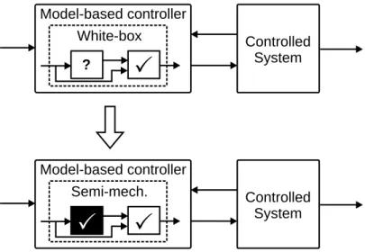
But it is not always possible to handle the model error effectively with the above mentioned compensation techniques. The nonlinear model-based controllers are usually based on first-principle models (white-box models), and there are situations when some parts of the white-box model are in fact not known or when the model uncertainty is significant (it will be illustrated in Chapter 5). Thus the application of model-based controllers may fail because sometimes the process is not known accurately enough. Moreover, the application of first-principle model in a model-based controller needs complete observability of states (state variables of the model), but on-line measuring of states may be complicated. If a state variable cannot be measured, one has to apply indirect measurement (calculation of a non-measured state variable from other measured variables using the model); however if the model is in- sufficient, indirect measurement will be inaccurate or even impossible. This work suggests including black-box elements as parts of white-box model, see Fig. 1.5, to handle such difficulties. White-box model only leans on mechanistic knowledge, so applying black-box modeling makes possible utilizing of

White-box Model-based controller

Controlled System

?

Semi-mech.

Model-based controller

Controlled System

Fig. 1.5. Semi-mechanistic modeling for control

(23)

1.5 Semi-mechanistic Modeling for Control 11 information form measurement data. This approach corresponds to the concept described in Sect. 1.1.

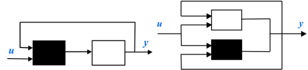
The proposed modeling approach is usually denoted as semi-mechanistic modeling. Thompson and Kramer [33] used the so-called parallel approach of semi-mechanistic modeling where the error between system output and white- box model is estimated by a neural network. They also described the serial approach where a neural network is used to model the unknown part of the model, see Fig. 1.6.

Fig. 1.6. Serial and parallel combinations of white and black box models

The proposed semi-mechanistic control corresponds to the serial semi- mechanistic model because the black-box element is a part of the white-box model. This approach will be presented in Chapter 5. It will be demonstrated how the white-box modeling approach (ﬁrst-principle model) and the black- box modeling approach (neural network) can be combined to achieve an effective nonlinear model-based controller. Chapter 5 will also concentrate on practical issues of semi-mechanistic modeling arising from model instability and nonlinearity, model uncertainty and measurement noise.

(24)

(25)

2 Interactive Optimization for Process Control and Design

System identification, process optimization and controller design are often for- mulated as optimization problems. The key element of the formalization of optimization problems is defining a cost function. Cost function is a mathematical function which represents the objectives of the expected solution, and the goal of optimization is usually to find the minima (or the maxima) of this function. However the cost function is explicitly/mathematically not available in some cases. Sometimes, the relationship among the design variables and objectives is so complex that the cost function cannot be defined, or even there is no point in defining a quantitative function. In this kind of situation, it is very difficult to apply the common optimization methods. This chapter presents an interactive optimization approach that allows process engineers to effectively apply their knowledge during the optimization procedure without the explicit formalization of this knowledge.

Most optimization techniques which work by improving a single solution step by step are not well-suited for interactive optimization, because one cannot use the gradient information of the psychological space of the user. The population based optimization algorithms seem to be more plausible, because they can be easily utilized for interactive optimization. In the ﬁrst part of this chapter, Sect. 2.1, the population based optimization algorithms are presented. After that, Sect. 2.2 presents the proposed interactive optimization framework. Finally, Sect. 2.3 presents the application examples.

2.1 Population Based Optimization

2.1.1 Evolutionary Algorithm

Evolutionary Algorithm (EA) [34–37] is a widely used population based it- erative optimization technique that mimics the process of natural selection.

EA works with apopulation of individuals, where every individual within the

(26)

population represents a particular solution. Every individual has a chromo- some that encodes the decision variables of the represented solution. Because a chromosome can contain a mixture of variable formats (numbers, symbols, and other structural parameters), EA can simultaneously optimize diverse types of variables. Every individual has a fitness value that expresses how good the solution is at solving the problem. Better solutions are assigned higher values of fitness than worse performing solutions. The key of EA is that the fitness also determines how successful the individual will be at propagating its genes (its code) to subsequent generations.

The population is evolved over generations to produce better solutions to the problem. The evolution is performed using a set of stochastic operators which manipulate the genetic code used to represent the potential solutions.

Evolutionary algorithm includes operators that select individuals for repro- duction, produce new individuals based on those selected, and determine the composition of the population at the subsequent generation. Table 2.1 out- lines a typical EA. The individuals are randomly initialized, then evolved from generation to generation by repeated applications of evaluation, selection, mutation, recombination and replacement.

Table 2.1. A typical evolutionary algorithm procedure EA;{

Initialize population;

Evaluate all individuals;

while (not terminate) do{ Select individuals;

Create oﬀsprings from selected individuals using Recombination and Mutation;

Evaluate oﬀspring;

Replace some old individuals by oﬀsprings;

} }

In the selection step, the algorithm selects the parents of the subsequent generation. The population is subjected to ”environmental pressure”. It means that the higher ﬁtness the individual has, the higher probability it is selected.

The most important selection methods are Tournament Selection, Fitness Ranking Selection and Fitness Proportional Selection.

• The Tournament Selection is a simple but eﬀective technique. In every tournament, two individuals are picked up randomly from the population, and the one with the higher ﬁtness value is selected.

• The Fitness Proportional Selection is an often applied technique. For each individual the selection probability is proportional to the ﬁtness of the individuals.

(27)

2.1 Population Based Optimization 15

• The Fitness Ranking Selection method uses a rank-based mechanism. The population is sorted by ﬁtness, and a linear ranking function allocates a rank value for every individual. The probability of selection is proportional to the normalized rank value of the individual.

After the selection of the parents, the new individuals of the subsequent generation (also called oﬀsprings) are created by recombination and mutation.

• The recombination (also called crossover) operator exchanges information between two selected individuals to create one or two new oﬀsprings.

• The mutation operator makes small, random changes to the chromosome of the selected individual.

The ﬁnal step in the evolutionary procedure is the replacement, when new individuals are inserted into the population, and old individuals are deleted.

Once the new generation has been constructed, the whole procedure is repeated until termination criterions satisfy.

Evolutionary Algorithm searches directly and represents potentially much greater efficiency than a totally random or enumerative search [38]. The main benefit of EA is that it can be applied to a wide range of problems without significant modification. However, it should be noted that EA has several im- plementations: Evolutionary Programming (EP), Evolutionary Strategy (ES), Genetic Algorithm (GA) and Genetic Programming (GP). The main differ- ence among them is that GA uses bit-string representation, ES uses real-valued representation, and GP uses symbolic representation. In the case of common process engineering optimization problems, the decision variables are usually real-valued, hence ES will be presented in the following subsection.

2.1.2 Evolutionary Strategy

Evolution Strategy was developed by Rechenberg [38], with selection, mutation, and a population of size one. Schwefel introduced recombination and populations with more than one individual, and provided a nice comparison of ES with more traditional optimization techniques [39]. The main elements of the ES algorithm are the followings:

Representation

Evolutionary Strategy typically searches in continuous space, i.e. it uses real- valued representation. Search points in ES aren-dimensional vectorsx∈Rⁿof object variables. To allow for a better adaptation to the objective functions’s topology, the object variables are accompanied by a set of so-called strategy parameters. The function of strategy variables is to control the mutation operator separately for each individual. So an ES-individual a_j = (x_j,σj)^T consists of two components, the object variablesxj = [xj,1, . . . , xj,n]^T and the strategy variables σj = [σ_j,₁, . . . , σ_j,n]^T.

(28)

Mutation

The mutation operator adds zj,i normal distributed random numbers to the objective variables:

xj,i =xj,i+zj,i, (2.1)

wherez_j,i =N(0, σ_j,i) is a normal distributed random number with σ_j,i standard deviation. Thus theσj strategy variables control the step size of standard deviations in the mutation for j-th individual. Before the object variables are changed by mutation operator, σj standard deviations are mutated using a multiplicative normally distributed process, that is

σ_j,i⁽^t⁾=σ_j,i⁽^t⁻¹⁾exp(τN(0,1) +τ N_i(0,1)), (2.2) with exp (τN(0,1)) as a global factor which allows an overall change of the mutability and exp(τ N_i(0,1)) allowing for individual changes of the mean step sizes σj,i. The τ and τ parameters can be interpreted in the sense of global learning rates. Schwefel suggests to set them as [40]:

τ = 1

√2n, τ = 1 2√

n. (2.3)

Recombination

Recombination in ES can be either sexual, where only two parents are involved in the creation of an offspring, or global, where up to the whole population con- tributes to a new offspring. Traditional recombination operators are discrete recombination, intermediate recombination, and geometric recombination, all existing in a sexual and global form. When F and M denote two randomly selected individuals from the µparent population, the following operators can be defined:

x_i =

⎧⎪

⎪⎨

⎪⎪

⎩

xF,i no recombination x_F,i or x_M,i discrete

(xF,i+xM,i)/2 intermediate µ

k=1x_K,i/µ global avarage

(2.4)

σ_i =

⎧⎪

⎪⎪

⎪⎨

⎪⎪

⎩

σ_F,i no recombination σF,i or xM,i discrete

(σ_F,i+σ_M,i)/2 intermediate (σ_F,iσ_M,i) geometric µ

k=1σK,i/µ global avarage

. (2.5)

Selection and Replacement

At ﬁrst, a certain number of individuals are selected from the current generation to be parent. The number of parents is usually denoted as µ. Then the

(29)

2.1 Population Based Optimization 17 algorithm composes a certain number of parent-pairs from the set of parents.

The number of parent-pairs is usually denoted as λ. The parent pairs are se- lected uniformly randomly. After that, the algorithm generates λ number of oﬀsprings using recombination and then mutation. Finally, the algorithm ar- ranges the subsequent generation. Evolutionary Strategy has two commonly- used replacement strategies: the (µ+λ) and the (µ, λ) strategy. The (µ+λ) strategy inserts the parents to the subsequent generation (it is elitist), while the (µ, λ) strategy does not conserve the parents. So when the (µ+λ) strategy is used, the size of population is µ+λ, while when the (µ, λ) strategy is used, the size of population is λ.

2.1.3 Particle Swarm Optimization

Particle Swarm Optimization (PSO) is a stochastic optimization technique developed by Eberhart and Kennedy in 1995 [41]. This optimization technique was inspired by swarm intelligence and evolutionary computation.

The PSO algorithm is initialized with a population of random potential solutions. In PSO, potential solutions are calledparticles. Every particle has a position which is ann-dimensional vectorx∈Rⁿ of object variables (nis the number of object variables). Object variables are generally normalized in such way that the problem space is a part of a n-dimensional unity cube. Every particle has a fitness value, which is a scalar valuef(x), wheref is the fitness function that must be maximized. The particles iteratively move through the problem space. Every particle has a velocity, v ∈ Rⁿ, which determines the movement of the particle. The movement of particles are influenced by the location of the best solutions achieved by the particle itself, p_j ∈Rⁿ for j-th particle, and by the whole population,g∈Rⁿ. These best solutions are called as particle-best and global-best. Table 2.2 shows the pseudo code of the PSO algorithm.

The advantage of PSO is its simplicity. In every iteration, the particles are updated by the following equations:

xj(t+ 1) =xj(t) +vj(t), (2.6) and

v_j(t+ 1) =w(t)v_j(t) +c₁u₁(p_j(t)−x_j(t))

+c₂u₂(g(t)−xj(t)) (2.7) where xj(t) is the j-th particle at t-th iteration, vj(t) is the velocity vector of j-th particle at t-th iteration, u ∈ [0,1) are uniformly distributed random numbers, c₁, c₂ are learning factors, w is an inertia weight parameter, pj(t) and g(t) are particle-best and global-best particles at t-th iteration.

The role of the w inertia weight in (2.7) is considered critical for the PSO’s convergence behavior. The inertia weight is employed to control the impact of the previous history of velocities on the current one. Accordingly,

(30)

Table 2.2. PSO algorithm procedure PSO; {

Initialize particle’s position xand velocity v;

Fort = 1 to t^max{ For j = 1 to N {

Calculate f(x_j) ﬁtness value;

iff(xj) > f(pj) then pj =xj; }

Choose the global best: g= arg maxf(p_j);

For j = 1 to N {

Update x_j particle position;

Calculate v_j particle velocity;

} } }

the parameter regulates the trade-off between the global and local exploration abilities of the swarm. A large inertia weight facilitates global exploration (searching new areas), while a small one tends to facilitate local exploration, i.e. fine-tuning the current search area. So it is worth making a compromise, e.g. w has high value at the first iteration, and then it decreases at every iteration:

w(t) = 0.4 + tmax−t

2·t_max , (2.8)

wheret_maxis the maximum number of iterations andtis the current iteration.

PSO shares many similarities with evolutionary computation. Both algorithms start with a group of a randomly generated population. Both update the population iteratively and search for the optimum with stochastic techniques. The main diﬀerence between them is in the information sharing mechanism. In EA, only the individuals of current generation share information with each other, and any individual has a chance to give out information to oth- ers. In PSO, actually not the current individuals share information with each other, but the individuals of previous generation (the optimal particles) give out information to the current ones. In other words, the information sharing is one-way in PSO.

2.1.4 Case-study

This section demonstrates how the above presented population based optimization approaches can be applied for process engineering problems through the case-study of temperature control of a continuously stirred tank reactor (CSTR). The model of the controlled system is taken from Sistu and Bequette [31]; see Sect. A.1 for details. For the temperature control of the process, it is advantageous to use cascade-control scheme, where the slave controller controls the jacket temperature, and the master controller controls

(31)

2.1 Population Based Optimization 19 the reactor temperature. According to the industrial practice, a PID (Pro- portional + Integral + Derivative) controller is in the master loop, and a P (Proportional) controller is in the slave-loop. Figure 2.1 illustrates the scheme of cascade control. The sample time was 0.2 min. It should be noted that the typical time constant of the system is about 0.1 h, so this is relatively small value.

Feed

Product P

PID Master

Controller

Slave Controller

Wreactor

W_jacket Treactor

T_jacket

Coolant

Fig. 2.1. Cascade control of CSTR

After the selection of the controller structure, the problem shrinks to ﬁnd the tuning parameters. The cascade PID-P controller has four tuning parameters: K^m, T_i^m, T_d^m and K^s, the ﬁrst three ones belong to the master controller, the last one belongs to the slave controller. There are several tuning procedures for linear systems (e.g. the Ziegler-Nicholson method or the Cohen-Coon method), but in this case these methods cannot be applied, because the controlled system is strongly nonlinear. So it is advantageous to employ a nonlinear optimization technique, where a cost function is minimized. In control engineering practice, the control error and the variation of manipulated variable are usually minimized. Thus the cost function was

fcost = 1 N

N k=1

abs(e(k)) +β 1 N

N k=1

abs(∆u(k)), (2.9) wheree(k) =w(k)−y(k) is the control error,N is the time of control experi- ment in sample instants,β = 50 is the weighting parameter. Theβ parameter was selected based on a heuristic rule: the eﬀect of variation of manipulated variable should be about ten per cent of the total cost.

Four diﬀerent optimization algorithms were applied for the tuning of controller:

1. Manual tuning by trial and error method.

(32)

2. Sequential Quadratic Programming (SQP). This is a classical nonlinear optimization method, in which a Quadratic Programming (QP) subprob- lem is solved at each iteration.

3. Evolutionary Strategy.

4. Particle Swarm Optimization.

The maximum number of function evaluations was limited to 1000. The SQP was initialized with the resulting point of a manual tuning. In the cases of ES and PSO, there are some parameters which must be adjusted. Table 2.3 shows the parameter-set used in this case-study.

Table 2.3. ES and PSO parameters

Parameter Value/Setting

ES:

Population size (λ) 40

Number of parents (µ) 10

Selection Fitness proportional

Replacement (µ+λ)

Recombination of design variables discrete sexual Recombination of strategy variables intermediate sexual

τ ^√¹_2n ^a

τ √¹

2√ n

a

PSO:

Population size 30 ^b

c1 2

c2 2

w at the start 0.95

w at the end 0.4

a n is the number of object variables, in this case-study: n= 4

b In ES λ−µ= 30 new individuals generated in every iteration, so it is30 for PSO

Table 2.4 shows the results. ES and SQP turned out to be the best algorithms for this case-study. One can see that ES found very similar tuning parameters as SQP, the integral and the derivative time constants are near the same, and the products of the master and slave controller gains are near the same too. (It should be noticed that, in this case-study, the change of master gain can be compensated by the change of slave gain if the product of them stay the same; although it is true only approximately.) The PSO algorithm found a diﬀerent solution which has a little bigger cost-value. After all, it can be said that ES and PSO provided similar optimization performance than SQP.

(33)

2.2 Population Based Interactive Optimization 21 Table 2.4. Numerical results of controller tuning (CSTR case-study)

Algorithm Optimum (K^m,Ti^m,Td^m,K^s) f^cost

Manual (20, 50, 1, -0.1) 0.181

SQP (48.1, 16.1, 2.7, -0.014) 0.156 ES (70.2, 17.7, 2.6, -0.0097) 0.155 PSO (68.2, 78.1, 0.91, -0.017) 0.167

2.2 Population Based Interactive Optimization

2.2.1 Introduction to Interactive Evolutionary Computation

The optimal operation of chemical processes typically requires simultaneous inspection of multiple objectives. These objectives may be very diverse, moreover they are typically in conflict with each other. For example, environmen- tally sound process requires more expensive operations and materials; energy economy leads to less efficiency. Consequently, when a process engineer for- mulates the optimization task, he/she must make decision which objectives are more important, which are not. In general, a process engineer uses his/her knowledge and experience to make this decision, and finally translates the whole problem to a quantitative cost function. This requires in-depth information concerning the various trade-offs and valuation of each individual objective. In addition, sometimes the objectives are explicitly/mathematically not available, or even there is no point in defining a quantitative cost function.

But even if the explicit mathematical formalization of the optimization problem is hard-to-obtain, a process engineer usually has an opinion on the optimal solution. Hence, it would be desirable to use a tool that allows process engineers to introduce theira priori problem-speciﬁc knowledge into optimization problems in an interactive way.

Interactive optimization needs a special optimization algorithm. Most optimization techniques which work by improving a single solution step by step are not well-suited for this approach, because one cannot use the gradient information of the psychological space of the user. The population based optimization algorithms seem to be more plausible. The population based algorithms can be easily utilized for interactive optimization, e.g. by replacing the ﬁtness function by a subjective evaluation. EA is especially ideal for interactive optimization, since the user can directly evaluate the ﬁtness of the potential solutions, for example, by ranking them. This approach become known as Interactive Evolutionary Computation (IEC).

2.2.2 IEC Framework for Process Engineering Problems

In contrast to the high number of IEC application examples (see Sect. 1.2), this approach has not been applied in process engineering so far. The interfacing of human ability with machine computation requires resolving some issues. This

(34)

is especially relevant problem in process engineering where the user should evaluate the performances of simulated solutions obtained on the basis of different models. This section presents an IEC framework which was developed for process engineering problems in MATLAB environment. The EAsy-IEC Toolbox was designed to be applicable for different types of optimization problems, e.g.: system identification, controller tuning, process optimization.

Thanks to the MATLAB environment, the toolbox can be used easily for various problems.

Selection Genotype

Phenotype

Replacement Crossover, mutation Fitness evaluation

Genotype

Phenotype

Selection Crossover, mutation

Replacement

Fig. 2.2. Classical IEC (left) and proposed IEC (right)

In general, IEC means an EA in which the fitness evaluation is based on subjective evaluation. In most works, it means the fitness function is simply replaced with a human user who ranks the individuals [1]. For example, he/she gives marks such as ”good”, ”acceptable”, ”non-acceptable”. The subjective rates given by the user are transformed to fitness values (or directly applied as fitness values) for the algorithmic part of IEC. This approach is simple, but this chapter suggests another approach for process engineering problems. In the proposed approach, the selection and replacement operators are replaced and there is not fitness evaluation, see Fig. 2.2. I suggest this approach instead of classical one, because I found that (for process engineering problems) this approach is more effective and comfortable.

In the developed toolbox, the user can analyze individuals based on the output of the target systems realized by the individuals. For example, the user can simultaneously analyze the numerical results with the plotted trajectories, proﬁles, etc. The number of displayed individuals is usually around seven, because it can be displayed spatially. Based on this visual inspection of the solutions and the analysis of some calculated numerical values and parameters, the user selects individuals that are used to formulate the next generation, and selects individuals that are replaced by oﬀsprings, i.e. see Fig. 2.3. The number of searching generations is limited to twenty generations due to the fatigue of human users.

In process engineering, one of the oldest optimization method is the heuristic method of trial-and-error. So the developed toolbox also allows active hu-