Bacterial Memetic Algorithm Trained Fuzzy System-Based Model of Single Weld Bead Geometry

(1)

Bacterial Memetic Algorithm Trained Fuzzy System-Based Model of Single Weld Bead Geometry

CSONGOR MÁRK HORVÁTH ^1,2, JÁNOS BOTZHEIM ¹, (Senior Member, IEEE), TRYGVE THOMESSEN², AND PÉTER KORONDI ¹, (Senior Member, IEEE)

1Department of Mechatronics, Optics and Mechanical Engineering Informatics, Faculty of Mechanical Engineering, Budapest University of Technology and Economics, 1111 Budapest, Hungary

2PPM Robotics AS, 7038 Trondheim, Norway

Corresponding author: Csongor Márk Horváth (hcsongorm@mogi.bme.hu)

This work was supported in part by PPM Robotics AS, in part by The Norwegian Research Council through the Virtual Presence in Remote Operation of Industrial Robot Systems and the Industrial Ph.D. Program under Grant 244972/O30, in part by the CoRoWeld Project through the User-Driven Research-Based Innovation Program under Grant 245691, in part by the MultiPass2020 Project through the SkatteFUNN Program under Grant 293141, in part by the NKFIH Hungary under Grant BME NC TKP2020, and in part by the BME Artificial Intelligence of NKFIH Hungary under Grant TKP2020 IE and Grant BME IE-MI-FM TKP2020. The work of János Botzheim was supported by the János Bolyai Research Scholarship of the Hungarian Academy of Science.

ABSTRACT This article presents a fuzzy system-based modeling approach to estimate the weld bead geometry (WBG) from the welding process variables (WPVs) and to achieve a specific weld bead shape.

The bacterial memetic algorithm (BMA) is applied to solve these problems in two different roles, as a supervised trainer, and as an optimizer. As a supervised trainer, the BMA is applied to tune two different WBG models. The bead geometry properties (BGP) model follows a traditional approach providing the WBG properties as outputs. The direct profile measurement (DPM) model describes the bead profiles points by a non-linear function realized in the form of fuzzy rules. As an optimizer, the BMA utilizes the developed fuzzy systems to find the solution sets of WPVs to acquire the desired WBG. The best performance is achieved by applying six rules in the BGP model and eleven rules in the DPM model. The results indicate that the normalized root means square error for the validation data set lies in the range of 0.40−1.56%

for the BGP model and 4.49−7.52% for the DPM model. The comparative analysis suggests that the BGP model estimates the BWG in a superior manner when several WPVs are altered. The developed fuzzy systems provide a tool for interpreting the effects of the WPVs. The developed optimizer provides multiple valid set of WPVs to produce the desired WBG, thus supporting the selection of those process variables in applications.

INDEX TERMS Bacterial memetic algorithm, fuzzy system, machine learning, TIG welding, weld bead geometry.

I. INTRODUCTION

Most of the automated welding systems were developed and used for mass production. Recently, the robotization of small series production gained more attention, primarily by small and medium-sized companies. The transition from manual to robotized welding requires the adaptation of the welder’s expertise to the automated system. However, this knowledge is mostly not available in a quantified format as precisely as needed to program the robotic welding system or estimate the weld bead geometry (WBG).

The associate editor coordinating the review of this manuscript and approving it for publication was Min Xia .

The Tungsten Inert Gas (TIG) welding method can produce solid and high-quality joints for a wide range of regular and more exotic types of metals [1]. Along with the welding process’s non-linear characteristics, the weld bead formation depends on the chemical compositions of the base and filler materials [2], [3]. The sulfur and oxygen content could vary in a wide range between the manufacturing batches, which influence the surface tension of the melted metal, an important factor defining the shape of the solidified surface [4], [5].

Furthermore, the deposition efficiency needs to be considered besides the inconsistent evaporation of the filler metal [6].

Consequently, a model-based approach is needed to achieve the requirements for the given material composition

(2)

and environment; and support the activities during the design and the execution of the welding process.

During the early 2000’s, optimization and modeling of welding processes mostly consisted of numerical [7] and statistical approaches [8]. However, in the last decade computational intelligence and machine learning became dominant [9], [10] due to the capability to solve complex and non-linear problems. Now they are providing a base for applications for future intelligent welding manufacturing [11]. Recently, WBG models and the related process controls gained attention in wire and arc additive manufacturing (WAAM) [12]–[15] and multi-pass welding (MPW) [16]–[18].

Most research studies of WBG modeling are focused on consumable electrode welding methods [12], [19]–[23] and flux activated TIG (A-TIG) without deposition [24]–[26].

Only a few study focus on TIG for stainless steel bead geometry [27]–[30], because TIG was traditionally used without deposition or on non-steel metals [31] to weld joints where the reinforcement is not utilized.

Numerical models provide deep analysis on the mechanical properties, residual stresses, distortion, and heat dis- tribution beside other internal properties of the welded workpiece [7], [32]–[34]. However, the bead shapes and the welding process variables (WPVs) are not considered, since they are provided as inputs to the finite element modeling and adjusted manually. The WPVs are adjusted until they provide the final product’s required properties, while the weld bead shapes are modeled by their simplified shape. The modeling neglects the challenges connected to the precise execution by including higher error margin and safety factors. The shape of the weld beads is an important factor in WAAM and MPW because controlled height and width are needed to ensure stable deposition [35]–[37]. Analytical models were developed to describe the bead shape [36], [38], [39], but those models were discussing the type of the fitting curve for the bead surface and its effect during overlapping.

Statistical methods are often used in the literature to provide the comparison base for different methods since their linear behavior is usually outperformed by methods capable of modeling the non-linear behavior [12], [21].

Computational intelligence (CI) techniques – such as artificial neural networks (ANN) [12], [22], [23], fuzzy inference systems (FS) [20], [24], [25], evolutionary algorithms (EA) [40], [41], and genetic programming (GP) [42] – are widely used to describe the WBG. However, due to their limitations [26], several hybrid computing techniques were developed [26], [32], including the adaptive neuro-fuzzy inference systems (ANFIS) [25], [26], [43] and the evolutionary fuzzy systems (EFS) [44], [45].

An important common feature of computational intelligence techniques is that they aim at acceptably suboptimal, usually, approximate solutions, while keeping the computational complexity at a tractable, usually low degree polynomial level. CI methods such as fuzzy systems and neural

networks are universal approximators [46], [47]. They can be transformed into each other, therefore any approach (or architecture) choice can be justified [48]–[50]. Kóczy showed that the Takagi-Sugeno-Kang (TSK) FS is asymptotically equiv- alent to the Mamdani FS model, and they can be transformed into each other [49].

The main advantage of choosing FS is the inference base, compared to the black-box behavior of the ANNs. Fuzzy systems provide human-like reasoning systems since their rule-based approach with a non-linear mapping of inputs offers an easily interpretable method, where the arguments leading to the conclusion can be assessed.

The FS method’s main drawback is to find the optimal definition of membership functions and define the sufficient number of rules. The fewer number of fuzzy rules may help understand the system’s decision-making, bringing the developed inference model closer to the person applying it in operation. Furthermore, the fuzzy inputs allow us to handle some degree of uncertainty in the input parameters, which happens in welding. In the overviewed literature, either high number (above 20 rules) [25], [26], [51] or manually defined fuzzy rules [24], [52] were applied to estimate one feature of the weld bead.

The tuning of the membership function parameters can be done by applying training algorithms [53], which allow the fuzzy systems to learn from data. In many different fields, the evolutionary algorithms are applied to design the fuzzy systems [44], [45], [54].

Several evolutionary optimization algorithms were developed, with the ability to solve and quasi-optimize problems with non-linear and discontinuous characteristics [55], [56]. The bacterial evolutionary algorithm (BEA) [57] is one of the possibilities that mimic bacterial rather than eukaryotic evolution among microbes. Each bacterium represents a solution to the original problem. In their mutation and the gene transfer operations, bacteria share chunks of their genes instead of performing neat crossover in chromosomes, which is the characteristic of the eukaryotes.

The main disadvantage of the classical evolutionary algorithms is the low convergence speed, thus long running time. However, combining them with gradient-based local search methods can utilize both methods’ advantages in the optimization process. This hybridization leads to memetic algorithms [58].

Bacterial Memetic Algorithm (BMA) [54] is a memetic algorithm, in which the bacterial technique is used instead of the classical genetic algorithm, and the Levenberg-Marquardt (LM) method [59], [60] is applied as local search. The BMA provides a competitive performance during optimization [61], [62] and supervised machine learning [62]

against genetic algorithm (GA) and particle swarm optimization (PSO) and their memetic versions. It has already been applied in several combinatorial optimization problems [61], [63], in continuous optimization tasks [64], and in supervised machine learning tasks such as fuzzy rule base

(3)

extraction [54] and training fuzzy neural networks [65].

However, the capabilities of BMA were not explored in welding or related technology yet.

II. PROBLEM DEFINITION

Precise positioning of weld beads is required to achieve a desirable weld join in welding, which is influenced by the weld bead shape during the deposition of multiple beads. The weld bead geometry is directly related to the WPVs, and the bead formation depends on the previously deposited beads’

shapes.

In small series productions, the tuning of the process could take up a significant amount of time and be done by trial and error method following internal standards; and carrying out experiments and laboratory analysis of the test workpieces.

This approach can be enhanced by a bi-directional model to describe the relationship between the process parameters and the resulting WBG to support the automated operation and the selection of the process variables.

Simulation and analytical models could also support the manufacturing process, where the WPVs and WBG are provided as inputs to the finite element modeling. The target WBG is modeled by simplified shapes and defined by manual calculations or numerical calculations to satisfy the criteria of the mechanical loads and stresses of the workpiece. The WBG and WPVs are adjusted until they provide the required properties of the final product. Mishra and DebRoy [32]

showed that a specific WBG could be produced by multiple combinations of the WPVs, even in the range qualified by the Welding Procedure Specification. A provided list of WPVs could allow to select the best combination fitting to the desired workpiece properties.

However, numerical modeling neglects the challenges connected to the precise execution by including higher error margin and safety factors. Proposing a model to estimate the bead geometry provides refined geometrical information to further evaluation of the mechanical properties and residual stresses in the workpiece. Therefore, such a model does not compete with the numerical models but complements them to define the WPVs and WBG.

As the industrial application aspect of the welding process is considered, three control parameters were selected in our approach, namely arc current (I), torch travel speed (v_t), and wire feed rate (vf). Arc voltage (U) was also recorded and included in the model as input since it had small fluc- tuation and a significant effect on the heat input. These four parameters will be referred to as Welding Process Vari- ables (WPVs). The examined parameters of the WBG were chosen as width (w), height (h), and cross-sectional area (A_B) and later referred to as Weld Bead Profile Properties (BPPs).

To describe the weld bead profiles, the second-order polynomial (parabola) fitting was chosen [36]. The parabola curves are reconstructed from thew,hparameters using the following equation:

y= −4 h

w²x²+h, (1)

wherex is the abscissa- andyis the ordinate of the profile points of the weld bead in the coordinate system in the cross section, according to the definition shown in Fig. 2. The parabola defined in Equation (1) does not contain the first orderxcomponent since the coefficient is zero because the origin of the coordinate system is in the focal point of the parabola.

The theoreticalA^d_Bcross-sectional area of the weld beads can be estimated according to Equation (2) by calculating the amount of the deposited weld metal:

A^d_B=ηdπD²_w 4 · vf

60v_t, (2)

whereηd represents the deposition efficiency, andD_wis the diameter of the feeding wire. The deposition efficiency is estimated by comparingA^d_Bcalculated value with the measured A^m_B value using the area under the curve on the measured profile (Eq. (3)).

A^m_B = Z w/2

−w/2

f(w,h) dx= 2wh

3 (3)

During our preliminary study, we found that the value of ηd is 0.955 with a standard deviation of 0.063 for the whole sample population, which is similar to a generally accepted (above 0.9) value [6]. Furthermore, the deposition efficiency decreases with the increase of arc current, which is interpreted as the result of a higher vaporization rate of the feed metal.

However, the sign and the degree of the deviations are not consistent, causing error propagation in multi-pass welding as the layered beads added on top of each other. On a given workpiece, the error is usually reduced by on-site adjustment of the torch position, and the welding parameters are set to as constant across several layers. Thus, we expect that an accurate model utilizing the measurement data can increase the accuracy of estimation of the WBG.

Furthermore, the review conducted by Vasudevan con- cluded that FSs are the best soft computing methods for control and monitoring of welding processes, and (GA) evolutionary algorithm-based models for WPV optimization [27].

This provided a motivation to utilize our method since it combines the advantages of both approaches.

The effectiveness of the BMA is emphasized by adapting it to our application in two different ways – developing a bead shape model and finding multiple optimal WPVs to achieve the target bead geometry. This method is unique since the BMA was not utilized in welding before or implemented for one problem with two roles (supervised trainer and optimizer). Furthermore, for the two separate tasks, two different methods are usually applied in the overviewed literature.

The specific aims of our study are to (i) provide a sufficient estimation model of the WBG by adopting the BMA to the welding application, where the FS-based model consists of a low number of fuzzy rules; and (ii) provide a decision support tool for selecting WPVs to achieve specific WBGs.

(4)

III. PROPOSED METHODS

Our proposed method provides a bead geometry model on single weld beads in a horizontal position using fuzzy systems, and an optimizer to retrieve a list of WPVs producing a specified WBG. These support the decision to chose a suitable set of WPV for simulation or execution. The developed FS provides a human-like reasoning system and a non- linear mapping of inputs to assess the arguments leading to the conclusion. The supervised training of the rule base and the optimization task are carried out by the same Bacterial Memetic Algorithm.

Our proposed method is capable of accepting not only the conventional main welding parameters but also the profile points of the weld beads directly, measured by a laser trian- gulation sensor allowing a broader range of applications than the traditional methods.

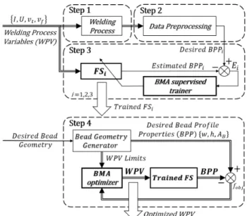
In the welding process modeling, BMA is used both as a supervised trainer and as an optimizer. Our method (Fig.1) can be broken down into the following four steps:

1) Welding data generation by TIG welding on 304L stainless steel

2) Welding data acquisition and preprocessingby the data processing framework

3) Welding model generationby tuning the membership functions of the fuzzy systems by BMA in order to infer the bead profile properties from the welding process variables

4) Welding design by BMA optimization of WPV in order to achieve the desired BPP resulting in a multiple set of WPV

The empirical model development is based on the welding experiments (Step 1), whose design is covered in the Sec.III- A, and utilize the second-order polynomial (parabola) fitting.

The generated data is preprocessed (Step 2) to provide the profile property information of weld bead cross sections for each trial, following the method described in Sec.III-B. The output of the preprocessing is the training patterns for the model development of the weld bead profile.

During the supervised training (Step 3, Sec. III-C), the BMA is utilized to tune the membership functions of the fuzzy systems. The bacterium’s chromosome encodes the breakpoints of the trapezoidal membership functions, and the evaluation of the bacteria is carried out by the Mamdani inference model [66]. The bacterium’s chromosome is modified to reduce the value of approximation error (E_i in Fig. 1), which is the difference between the estimated and the desired BPP value in thei-th training pattern. The correlation between the WPVs and the BPPs is realized in two separate models.

The first approach, the Bead Geometry Properties (BGP) model (Sec.III-D), is a more conventional method to model a direct relation between the WPVs and the BPPs in three parallel fuzzy rule bases. The second approach is the Direct Profile Measurements (DPM) model (Sec.III-E), which is the extension of the BGP model. It contains a single fuzzy rule base to reconstruct the weld bead shape from profile points;

FIGURE 1. Overview of the proposed method’s structure.

then, the BPPs are acquired as the result of the postprocessing.

As Step 4, the BMA is used again, now as an optimizer, incorporating the BGP model to optimize the WPVs to achieve the targeted weld bead geometry (Sec.III-F). Both the fitness of the models and the results of the optimization were validated through experiments.

The application of BMA in Step 3 and Step 4 differs in a few details, such as the encoded information in the bacteria’s genes, the evaluation method, and the update process in the Levenberg-Marquardt algorithm. In the optimizer role, the bacterium encodes the WPVs, and the evaluation is based on the value of the single objective function. According to their gradient vector, the WPVs are modified with their direct effect on the objective function in the iterations between the generations. In comparison, in the supervised trainer role of the BMA, the bacteria’s chromosomes encode a complete set of fuzzy rules. The parameters of the rule’s membership functions are tuned in the process. During the evaluation of a bacterium, the estimated and the desired response of the fuzzy system is calculated as provided in the training patterns, giving the algorithm a multi-objective characteristics which is transformed into a single-objective optimization with uniform weights. Therefore, the gradient is represented as a Jacobi matrix instead of a gradient vector. The detailed discussion will be given of the implemented Levenberg- Marquardt algorithm in both cases in the corresponding sections.

A. EXPERIMENT DESIGN AND EXECUTION

A bead-on-plate welding experiment was carried out to create an estimation model of the weld bead profile (Step 1).

Figure 2 shows a measured cross-section of a weld bead, incorporated visualization of the BPPs, and the expected results of the proposed models.

(5)

FIGURE 2. A weld bead cross-section as the result of the measurements and the models.

The base metal is 20mmthick 304L steel with 3mmclad welded with the same 1.2mmdiameter Böhler 13/4-IG filler material as used to produce the weld bead. The experiment was executed with a regulated constant 12 V, 2.4 mm arc gap in PA welding position, 40^◦C preheating temperature.

An E3 tungsten electrode with rare earth mixed oxides of 3.2mmdiameter and 60^◦cone angle was used. Pure Argon gas with a flow rate of 12−14L/minprovided the shielding.

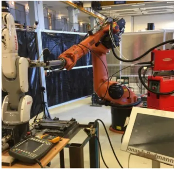
The experiment was carried out in the welding cell shown in Figure3by aKuka KR-30-3and aNACHI MZ-07industrial robot arms, using a MagicWave 5000 JOB welding power source, and a custom controller software.

TABLE 1. Definition of input process parameters and their levels.

Taguchi design [67] was applied to design the experiment using anL25(5³) layout as shown in Table1. Each trial was carried out twice, and each produced a 100 mmlong weld bead. The WPVs’ minimum and maximum values of the parameters were selected to comply with theWelding Process Specification, provided by our industrial partner. Unfortu- nately, not all samples provided usable data due to welding failures. Our design considered non-optimal settings; thus, high heat input was applied in the failed tests with a low feed rate and vice versa; consequently, these settings are not suitable for industrial applications. At the end of the modeling process, welding data from the N_trial = 42 trials were included for the training, which was the result of 21 different WPV combinations (Training data sets in Table2). A similar experiment was carried out to prepare the weld beads for

FIGURE 3. Robotic welding cell, where the experiments were carried out.

the independent validation. Seven WPVs combinations were selected arbitrarily from different regions of the parameter window, and then each welding trial was performed twice (Validation data sets in Table2).

After each finished welding sequence, the weld beads’

surface was recorded by a M2DW 160/40 Line Laser Tri- angulation Sensor (LTS). Each weld bead was measured by 0.1 mmincrements along the weld line containing ca. 100 data points per profiles, which supplied theRSPraw scanned profiles as cross-sectional data for further data processing.

The first and last fifth of the weld beads were neglected; thus, only the stabilized cross-sectional area was considered with an effective length of 60mm.

B. WELD BEAD PROFILE DATA ACQUISITION AND PREPROCESSING

The profile data of the weld beads were preprocessed (Step 2. in Fig1) in a framework developed in LabVIEW^TM. The pseudo-code of the whole process is shown in Algo- rithm 1. The framework requires the measurement profile data from the LTS sensor (SMP), the WPVs from each trial, and the trajectory information of the welding robot system (RSP). As the first step, the required information was combined into weld bead profile data (CPD); thus, each cross-section of the weld beads contained aligned position information from the robot system with the corresponding actual welding parameters and measurement points.

The weld bead measurements were taken before and after the welding sections using the LTS scanner, producing the cross-sectional measurements along the weld line with a 0.1 mm incremental steps. Five consecutive CPD cross- section measurements were combined into oneS profile for

(6)

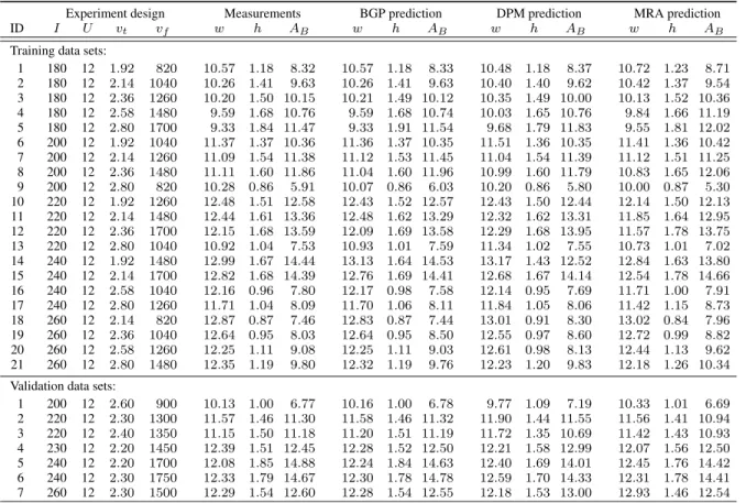
TABLE 2. Mean values of the measurements and the predicted values of the proposed models. Dimensions of the experiment design:Iarc current [A],U arc voltage [V],v_ttorch travel speed [mm/s],v_f wire feed rate [mm/min]. Dimensions of the weld bead geometry:wbead width [mm],hbead height [mm], bead area [mm²].

each trial to reduce the noise of the LTS and the WPV measurements. This resulted inS = 120 cross-sections for each trial, containing ca. 100 data points per profile. How- ever, five percent of the cross-sections were discarded due to failed measurements caused by the material’s locally high reflection.

During the data processing, each profile of each weld bead was filtered for noise, aligned to the horizontal position, and segmented to identify the weld bead. The segmentation provided the data points for the weld bead profiles and the substrate segment. In our case, the substrate segment was the flat base metal, but profile sections from other trials also appeared; however, they were discarded. The fitting method was chosen as the second-order polynomial, described in Eq. (1), to generate the BPP for the training and validation.

After the analysis, two sets of training patterns were generated in the Multiple-Input-Single-Output format. The first set was used for the BGP model tuning, consisting of three separated sets for the weld bead profile parameters (w,h,AB) with the input parameters of (U,I, vt,vf) for each cross- section, 4795 cross-sections altogether. The other set was used for DPM model tuning, consisting of the weld bead profile points (Y) and the input parameters of (X,U,I,v_t, v_f) creating the 487 286 training patterns.

The overall measurement process time depends on the number of completed O_pproc pre-processings of the bead

profiles calculated as:

Opproc=Ntrial·S (4)

The validation sets were processed in the same way as the training patterns. The welding trials contained seven arbi- trary WPV combinations with two parallel executions. The weld beads’ length was 100mm, and the first and last sections were discarded again. Altogether 1608 cross-sections were used with the same amount of validation patterns for the BGP model and 158 548 validation patterns for the DPM model.

C. BACTERIAL MEMETIC ALGORITHM FOR TRAINING FUZZY SYSTEMS

In order to define the fuzzy systems for the weld bead models, we applied the BMA as a supervised trainer (Step 3.

in Fig.1) on theNpatterntraining patterns [54]. In this case, the BMA minimizes the cumulative error between the output of the training patterns and the output of the fuzzy rule bases by adjusting the breakpoints of the fuzzy rules’ trape- zoids, encoded into the bacterium’s chromosome [54]. The evaluation of the bacteria is carried out by the Mamdani Inference Model [66], and the result is given as the Sum of Squared Error (SSE) between the model output and the desired output of the patterns. This evaluation is used in all steps of the BMA.

(7)

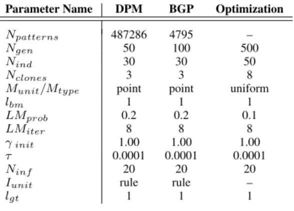
The BMA consists of four main steps, first the random generation of the initial population, then the three main operations are performed in each generation. These three operations are the bacterial mutation (BM), the local search by the Levenberg-Marquardt method (LM), and the gene transfer (GT). The pseudo-code of the BMA method is shown in Algorithm 2, and the applied meta parameters are listed in Table 3. These meta-parameters are selected according to the problem’s size to provide the balance between the required computational time and residual error of the estimation. The parameter settings are deducted from the preliminary experiments, based on the experience gained from the earlier application of the BMA on other problems [54], [64], [65].

TheRirules in the fuzzy system are given in the following form:

Ri: IFx1=Ai,1and . . . andxn=Ai,nTHENy=Bi, where x = (x₁, . . .xn) is the input vector, y is the output, A_i = (A_i_,₁. . .A_i_,_n) is the antecedent parameter vector, and B_i is the consequent parts in the i-th rule.

The rule base is defined to cover the whole interpretation interval of the input variables to provide a valid inference result. The trapezoidal membership functions can be written as:

µA_ij(xj)=









 x_j−a_ij

b_ij−a_ij, ifaij<xj≤bij

1, ifb_ij<x_j≤c_ij d_ij−x_j

dij−cij

, ifc_ij<x_j≤d_ij 0, otherwise,

(5)

Algorithm 1Processing of the Bead Profile Measurements Require: RawScannedProfiles:RSPprofile measurements Require: WeldingProcessVariables:WPV parameters Require: RobotSystemParameters:RSPparameters Require: N_trial,N_profile[ID_trial]

CombineRSP,WPV, andRSPintoCPDcombined profiles data

forEach trialdo

CombinefiveCPDprofiles into oneSprofile forEachSprofiledo

Filter measurement and correct errors Profile Segmentation

Curve fitting

Acquire profile properties end for

end for

ExportP1 Training patterns (Weld Bead Profile Proper- ties)

ExportP2 Training patterns (Profile Points of the Bead Segments)

whereaij ≤ bij ≤ cij ≤ dij denote the four breakpoints of the membership function of thei-th rule and the j-th input variable. Theai,bi,ci,divalues belong to the output membership function in thei-th rule. As in the original Mamdani algorithm, theminimumoperator is used as the t-norm in the inference mechanism meaning that the degree of matching of thei-th rule in the case of anN_input-dimensional crispxinput vector is:

wi=

Ninput

min

j=1 µA_ij(xj). (6)

The output of the fuzzy inference is defined asmaximum aggregation. The defuzzification is calculated by theCenter of Sumstechnique, which can be given in the explicit formula as shown in Equation (7), where the number of rules isN_rule, andNinput is the number of the input dimensions.

The operation of the BMA starts with the generation of the initial population, generatingNind random individuals with the restriction to maintain the trapezoidal characteristics of the membership functions in the fuzzy rules. The number of rules (N_rule) is defined beforehand and set to a low number to avoid the model overfitting. The total number of the created membership functions isN_ind · (N_input +1)·N_rule whereN_input = 4 is the number of input variables and each membership function has four parameters. In the iteration phase of the algorithm, the bacterial mutation, local search, and gene transfer operations are performed until the number of generations (N_gen) is reached.

Let us definek as the iteration variable, vector b_k (the bacterium) contains all the parameters of the membership functions, andx^(p)as thep-th training pattern’s input vector.

Here, the evaluation of the bacterium is carried out as E(b_k)= ||e_k||²

2, (8)

the 2-norm sum of squared error of the desired and model’s output values, where the elements of thee_k vector are calculated as

e_k =h e^(p)_k i

=h

d^(p)−y_k(b_k,x^(p))i

, (9)

where d^(p) is the desired value given in the p-th training pattern, andy_k(b_k,x^(p)) is the output value for thex^(p)inputs provided by fuzzy system encoded in theb_k bacteria.

Algorithm 2Bacterial Memetic Algorithm Require: Patterns:Npatternpatterns

Require: Parameters :Nind,Ngen,Nrule,Nclone,lbm,Munit, LMprob,LMiter,γinit,τ,Ninf,lgt,Iunit

Create initial population forgen=1 toNgendo

forind =1 toN_inddo Bacterial mutation

Levenberg-Marquardt algorithm end for

Gene transfer in the population end for

(8)

TABLE 3. Parameters of the BMA.

1) BACTERIAL MUTATION

The bacterial mutation is applied one by one to each bacterium (Algorithm 3). First, Nclone clones of the rule base are generated, which are then subjects of random changes in their genes according to the mutation unit (M_unit), which can either be a breakpoint of the trapezoid, an entire trapezoid, or an entire rule. The number of modified genes during this mutation is given by the mutation segment length (l_bm) parameter of the algorithm. All clones are evaluated, and the best individual transfers the mutated part into the other individuals. In the end, only the best rule base is kept. The bacterial mutation is repeatedN_segmenttimes, whereN_segment depends onM_unitandl_bm, and its value is 4·N_rule·(N_input+ 1)/l_bmin the case of point mutation.

In each generation, the computational cost of the bacterial mutation operator can be defined according to theO_BM num-

Algorithm 3Bacterial Mutation

Require: Parameters:N_ind,N_clone,l_bm,M_unit Create (N_clone+1) clones ofBacterium SetN_segment =4·N_rule·(N_input +1)/l_bm fori=1 toN_segmentdo

Selectlbmyet unmutated random gene

forj=1 toNclonedoMutate selected gene inClonej

end for

forj=1 toNclone+1doEvaluateClonejusing Eq. (8) end for

SelectBestClone

Transfer best clone’s gene to all clones end for

SetBacterium=BestClone

ber of fitness function calls:

O_BM =N_ind·N_clone·N_segment. (10) 2) LEVENBERG-MARQUARDT ALGORITHM

After the bacterial mutation step, the Levenberg-Marquardt algorithm (Algorithm4) is used for each individual to solve the minimization problem.

The local search was carried out with aLMproblocal search probability for each individual, maximumLMiter number of iteration steps until theτ terminal condition is met.

Let denoteJ(b_k), as the Jacobian matrix ofb_k bacterium:

J(b_k)=

"

∂yk(b_k,x^(p))

∂b^T_k

#

(11) Equation (11) expresses, that each row of theJ(b_k) matrix contains the partial derivatives of the output calculated by the Mamdani inference method for the givenx^(p)input pattern according to theb_k bacterium encoded parameters. The detailed calculations of derivatives of theJ(b_k), are given in [54].

The calculation of the Levenberg-Marquardt s_k update vector is carried out as

s_k = −(J^T(b_k)J(b_k)+γkI)⁻¹J^T(b_k)e_k, (12) whereγkis the bravery factor initially set to positive, andIis the identity matrix. The value ofγk controls both the search direction and the magnitude of the update. If the value ofγk

converges towards zero, then the algorithm applies the Gauss- Newton method, if towards infinite, then the algorithm gives the steepest descent approach.

Algorithm 4Levenberg-Marquardt Algorithm Require: Patterns:N_patternpatterns

Require: Parameters:LM_prob,LM_iter,γinit,τ ifRandom(probability)<LMprobthenk=1

whilek<LMiter andτk > τdo

Calculatesk update vector as Eq. (12) Calculaterk trust region as Eq. (14) Calculateγk+1bravery factor as Eq. (13) Evaluate the update vector’s effect as Eq. (15) Calculateτkstopping criteria

k=k+1 end while end if

y(x)= 1 3

Nrule

P

i=1

3w_i(d_i²−a²_i)(1−w_i)+3w²_i(c_id_i−a_ib_i)+w³_i(c_i−d_i+a_i−b_i)(c_i−d_i−a_i+b_i)

Nrule

P

i=1

2w_i(d_i−a_i)+w²_i(c_i+a_i−d_i−b_i)

. (7)

(9)

Algorithm 5Gene Transfer

Require: Population:N_indBacterium Require: Parameters:N_ind,N_inf,l_gt,I_unit

fori=1 toN_inf do

Ascending order of the population according to Eq. (8) SrcBact=Random(0, . . . ,N_ind/2−1)

DestBact=Random(Nind/2, . . . ,Nind) Select randomlgt genes

Transfer the selected genes fromSrcBacttoDestBact end for

The value of parameterγkis adjusted dynamically depending on the value ofr_k trust region:

γk+1=







4γk, ifr_k <0.25 γk/2, ifr_k >0.75 γk, otherwise

(13)

The value ofr_kfor the supervised training is calculated as:

r_k = E(b_k)−E(b_k+s_k) E(b_k)− ||J(b_k)s_k+e_k||²

2

(14) The evaluation of the local search success is verified as

b_k+1=

(b_k+s_k, ifEval(b_k+s_k)<Eval(b_k)

b_k, otherwise (15)

Evalfunction meansEas defined in Eq. (8) during the supervised training. Equation (15) is interpreted as if the update vector modifies the bacterium towards the local minimum then we carry on with the new value, otherwise it is left unchanged. The iterations stops if maximumLM_iternumber is reached or theτk < τ complex stopping criteria [54] is fulfilled.

The averageO_LM computational cost describing the number of fitness calls of the Levenberg-Marquardt algorithm in one generation is:

OLM =Nind·LMprob·LMiter, (16) where an additional (4·Nrule·(Ninput+1))³computational cost is required for each fitness function call, due to the pseudo- inverse calculation of theJ(b_k) Jacobian matrix.

3) GENE TRANSFER

The last operation in a generation is the horizontal gene transfer (Algorithm5), allowing the recombination of genetic information between two bacteria. This operation is per- formedN_inf (number of infections) times in one generation.

First, the population is split into two halves according to the fitness values. Then, a randomly chosen, better bacteria overwrites a randomly chosen, worse one’s gene with its own.

Here a gene (infection unit (I_unit)) means either a breakpoint of the trapezoid, or an entire trapezoid, or an entire rule. The l_gt parameter means the infection segment length, i.e., the number of overwritten genes.

TheOGTcomputational cost of the gene transfer operator in one generation is:

O_GT =N_ind·log(N_ind)+N_inf (17) The totalO_BMA computational cost of the BMA can be estimated as:

O_BMA=(O_BM +O_LM+O_GT)·N_gen, (18) which is the number of fitness function calls during run time.

The number of executions of the Mamdani inference process (Eq. (7) is:

O_FS=O_BMA·N_pattern. (19)

D. BEAD GEOMETRY PROPERTIES MODEL

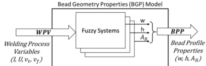
The BGP model is following a classical approach for recon- structing the weld bead shape. The model provides a direct relation between the WPVs and BPPs, where a dedicated fuzzy system is defined for each property. Thew,h, andA_B parameters are depending on the fitting model applied during the data preprocessing. The scheme of the model is shown in Fig.4. The bead profiles, as parabola curves are reconstructed from thew,hparameters using the Equation (1).

FIGURE 4. Schematic structure of the bead geometry properties model.

The computational cost of building the BGP model is given according to the cost of the utilized fuzzy systems:

O_BGP=3·O_FS (20) Since the BPP parameters are detached from each other, the BGP model’s fuzzy systems can be separately used to estimate only the required BPPs in an application where the full shape is not needed.

E. DIRECT PROFILE MEASUREMENTS MODEL

The DPM model (Fig.5) is an extended version of the BGP model and provides they=f(x,WPVs) non-linear function.

The central part of the model is the single fuzzy system, where the WPVs are extended with the bead profile’s abscissa vector to estimate the corresponding ordinate directly for each profile point. The training patterns are generated from the measuredN_point profile points of the cross-sections after preprocessing, following the process described in Sec.III-B.

The corresponding BPPs are extracted during the profile postprocessing, using the same parabola fitting principles as discussed in the BGP model development. Since the DPM model enables us to maintain the curve fitting model outside

(10)

the training, we can apply further fitting models and other considered limitations. This could allow examining different curve fitting functions such as cosine, arc, or ellipsoid, and also extending the model beyond the flat plate experiments as the subject of further research.

FIGURE 5. Schematic structure of the direct profile measurement model.

The computational cost of building the DPM model isO_FS, but theN_patternnumber of patterns is much higher than in the case of BGP model (see Table3). However, the cost of the utilization of the DPM model is:

ODPM =Npoint·OFS, (21)

where N_point is defined by the required resolution of the estimated bead profile, with an additional cost of curve fitting to retract the BPPs.

F. OPTIMIZING THE WELDING PROCESS VARIABLES It was previously shown how the BMA was used to tune the fuzzy systems during the model development. In this section, the BMA is utilized as an optimizer [64] (Step 4. Fig.1) to identify different sets of WPVs to achieve the desired BPP by minimizing the value of the fobj objective function on the predefined interpretation intervals. The evaluation of the fobj includes the calculation of the fuzzy system response for each BPP. The target BPPs are defined by manual calculations or numerical calculations to satisfy the criteria of the mechanical loads and stresses of the workpiece. The bacteria encode the WPVs in their chromosomes. During the evaluation of the bacteria – which is used in all BMA steps – the bacteria’s response is calculated by the BGP model for each target value, and the result is given as the value of the f_obj.

In our approach, the computational task involved the following three steps:

1) Selection of target weld geometryfrom the available sets of values ofw,h,A_B

2) Running the optimization processto obtain multiple combinations of WPVs (Algorithm6)

3) Verification of the producedresults for each target value

It was shown in the literature [32] that multiple combinations of welding process variables could be estimated to achieve a target weld bead geometry. On the full range of the search window, the BMA optimizer provided almost identical solutions at the global minimum. Therefore, each input variable’s search window was segmented into N_subint = 5

intervals, and the full range was left for the other inputs. For each segmented search window, multipleNrun=3 evaluation runs were performed, then the averaged values of WPVs contained in the best bacteria were given as the result of that segment. Due to the overlapping search windows, multiple identical WPV sets occurred and were unified to provide the final list of solutions.

At the start of the BMA operation, an initial population of 50 bacteria was defined. The meta parameters of the algorithm are presented in Table3. Each bacterium in the population contains a set of randomly chosen WPVs. Values of the welding process variablesI,U,v_t andv_f were chosen in the range of 160.0−280.0A, 10.50−13.50V, 1.80− 3.40 mm/s, and 600 −2100 mm/min, respectively. Since in the application of BMA as an optimizer, no training sets were applied, the course of the algorithm is different, and the evaluations carried out on vectors instead of matrices. The evaluation is replaced by calculating the value of the single- objectivef_objfunction for three weld bead profile properties:

f_obj=λ1

w^p w^t–1

2

+λ2

h^p h^t–1

2

+λ3

A^p_B A^t_B–1

!2

, (22)

whereλi are the weights of the objectives, set to constant 0.6, 0.3, 0.1, respectively, upper index p represents the BPP value estimated by the BGP model, andt represents the desired target BPP. The target BPP of the desired bead geometry is obtained experimentally; thus, the target values would maintain a realistic ratio to each other. The verification of the computed solutions requires that the set of WPVs used to produce the weld should appear with a small deviation in the provided solutions.

Further modifications are applied in the Levenberg- Marquardt algorithm, where the steps remain unchanged, but the definitions ofr_k, ands_kare updated. The update vector is defined for a given bacterium at thek-th iteration as:

s_k = −

g(b_k)⊗g(b_k)^T +γkI−1

g(b_k), (23)

Algorithm 6Welding Process Parameter Optimizer

Require: Optimizer Parameters : Intervals, N_run, RuleBases,BPP_target,N_subint,N_input

Require: BMA Parameters :Nind,Ngen,Nclone,lbm,Munit, LMprob,LMiter,γinit,τ,Ninf,lgt

Define intervals and number of runs fori=1 toNinputdo

forsub=1 toNsubintdo Set recent sub-interval forrun=1 toN_rundo

Bacterial memetic algorithm end for

end for end for

Remove duplicates and miss-matches

(11)

where g = ∇fobj is the gradient vector, approximated by second-order accurate, central finite differences;⊗stands for the dyadic product of two vectors, and the other parameters are defined as in Eq. (12). The value ofr_kfor the optimization is calculated as:

r_k =fobj(b_k+s_k)−fobj(b_k)

g(b_k)^Ts_k (24)

Value ofγk still depends onrk as given in Eq. (13). The bacteriumb_k+1is given according to Eq. (15), where theEval function is calculated as the fobj. The iteration stops if the stopping criteriaτk = ||g(b_k)||₂< τis fulfilled or maximum LMiternumber is reached.

In the optimizer version of the BMA the additional computational cost of O_LM is decreased to (N_input)³ due to the different amount of calculations needed for thes_k in the two roles. The computation cost, i.e. the number of objective function calls (Eq. (22)) in the BMA optimizer is:

Oopt=Ninput·Nsubint·Nrun·OBMA, (25) due to the segmentation of the intervals of the input parameters. The WPV sets encoded in the bacterium’s chromosome were improved through the generations using the BMA (Sec.III-C, meta parameters in Table3), monitored by calculating the f_obj objective function values for each set of bacteria. A bacterium with a lowf_objvalue indicates that the WPVs in it produces a target geometry with a small deviation from the estimated geometry.

IV. RESULTS AND DISCUSSION

In this section, the results of the development work will be discussed, including the overview of the main findings of the weld bead profile modeling, the comparison with other published models, and the evaluation of the WPVs optimization. The computations were carried out on a PC using an Intel^R Core^TM i7-5820K Processor at 3.30 GHz and an NVIDIA GeForce^R GTX 970 graphics card. The trained models’ performance was evaluated by comparing the estimated and the measured values to define the goodness of the fitting using the root mean square error (RMSE); the normalized RMSE value to the output range (NRMSE); and the RPearson product-moment correlation coefficient. The normalization was carried out on the range of the measured propertiesw: 8.82−13.75mm, h: 0.93−2.19mm, and A_B:6.18−16.88mm².

The evaluation of fitting was performed on an independent validation data set to avoid the models’ overfitting, and the data was preprocessed in the same way as the training patterns. The comparison to other models includes models from the literature and a multiple regression analysis (MRA) model on the available data set, see in Sec.IV-B.

A. EVALUATION OF THE TRAINED MODELS

The training of the fuzzy systems of the BGP model was carried out on multiple numbers of rules between two and seven. The required calculation time depended on the number

TABLE 4.Comparison of the RMSE and NRMSE values between the training and validation data for the BGP model.

TABLE 5.Comparison of the RMSE and NRMSE values between the training and validation data for the DPM model.

of rules. As long as for two rules (R2), one generation for each parameter was calculated just under 2srequiring 191s for the whole calculation. For six rules (R6), one generation is calculated 5s, and the whole calculation took 501s; for seven rules (R7), the run times were 6sand about 10min. The response time of the model for the input parameter change is approximately 5ms.

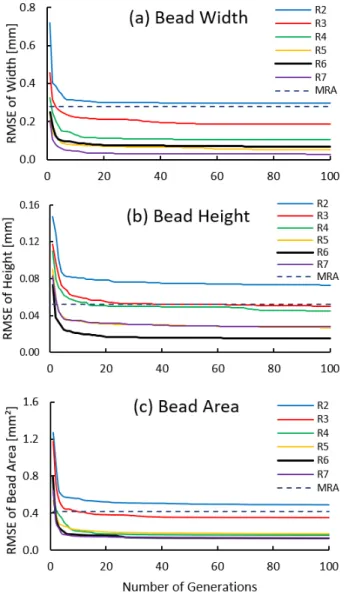
Table 4 shows the comparison of the RMSE values obtained on the training and the validation data for the property estimation of weld bead profiles. It can be seen that the roughest estimation is given by the FS with two rules. Its estimation accuracy is similar to the MRA model. However, when the number of rules increases, the estimation accuracy is also increasing, and the best result for the validation data was obtained using six rules (R6) for all three geometry properties. In the case of estimating the bead width, R6 and R7 provide a similar result, but the difference is in the last digit; thus, the lower number of rules is preferred. Figure6 illustrates the evolutionary process for each BPP to compare

(12)

FIGURE 6. Evolutionary process with different number of rules for each Bead Profile Property (BPP) and comparison to the MRA model output (RMSE values).

the RMSE values over the generations. In each case, the R6 is among the best performers, and the estimation accuracy increases with the number of applied rules. Furthermore, the steepest increase in the fitting is observed in the first tens of generation, with a slow but steady increase during the later generations. These results support the quick convergence of the BMA towards the global optimum and increase accuracy as long as the algorithm is running.

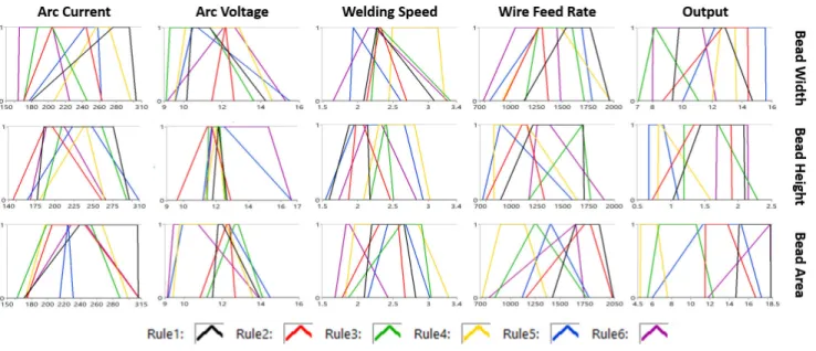
The rules of the BGP model for each BPP are shown in Fig.7and tabulated in Table6. Each row represents one FS estimating a BPP, and the membership functions of the same rule are marked by the same color.

The interpretation of the rule bases shows that the weld beads’ width is not affected by the amount of the deposited metal, but the applied arc current and torch travel speed. The weld bead height has a base value, which is independent of the WPVs changes, but the additional gain affected mostly the

applied material (increase) and the applied current (decrease).

The rule base shows that the weld bead area calculation depends on the variation in the torch travel speed and the wire feed rate.

These findings strengthen the applicability of the proposed method since it provided a reasoning base from experimental data, providing similar assumptions that are part of an experienced welder’s knowledge base. Therefore, these rules can be used in training or supporting a robot cell’s commissioning when monitoring the degree of changes in the weld geometry while tuning the WPVs. Another possible application is in the WPV optimization to achieve a predefined bead geometry.

In Fig.8, the correlation between the estimated and the measured values is illustrated for the models with the best performing rule sets. The results are compared with the expected values and the estimated values of the reference MRA model. In the case of the BGP model, correlation coefficients for the training are 0.9970, 0.9970, and 0.9975, respectively, with an RMSE value of 0.0683, 0.0153 and, 0.1245. Consequently, the estimated and the measured values correlate with a high degree, and the approximation accuracy in the training is above 98.5 percent. Similarly, the validation set’s correlation coefficients are 0.9903,0.9997, and 0.9984, showing a similar good correlation. The RMSE values are 0.0769, 0.0054, and 0.1082, meaning that the model estimates unknown values within its application range under one percent of the average error for each parameter.

The training of the DPM model required a higher number of fuzzy rules but one system instead of three since it created an estimation model for the curve fitting itself. The training was also carried out with a various number of rules as their RMSE values are presented in Table 5. The best- fitting rule number was found as six (R6) for estimatingw with a 5.3 and 6.0 percent of average error for the training and the validation set. Eleven rules (R11) provided the best estimations for h and A_B, with an average approximation accuracy of 95 percent. The calculation required 215minfor up to eight rules, 392min for nine rules (R9), and 646min for eleven rules (R11) in total for the 50 generations on the same hardware used for the BGP model. The response time of the model for the input parameter change is approximately 8ms. A similar execution time was experienced up to eight rules (but as the number of rules increased, a raise in required time was observed) since the model calculation utilized the advantages of the GPU provided parallel programming.

As Fig. 8 shows, a good agreement exists between the actual values and the estimated parameters of the weld bead profiles. The BPPs of the training data set were estimated with the correlation coefficients of 0.9734, 0.9649, and 0.9528.

Similarly, 0.9001, 0.9069, and 0.9604 values were achieved for the validation set. As observed, the width estimation showed the best result at six rules, and the estimation was overfitted on the training data as the rule number increased.

The height and bead area approximation accuracy increased with the number of applied rules.

(13)

FIGURE 7. Rule bases of the BGP model to estimate BPPs from WPVs.

TABLE 6. Mamdani Fuzzy system definitions for the bead profile parameters by the BGP model.

The comparison of the two models in both cases showed good fitness for the training and the verification data sets.

However, the DPM model provided a bit of noisier output.

The correlation coefficients for the verification sets were slightly worse than that of the training sets, which can be explained by the sensitivity of curve-fitting on the width and height parameters during the data preprocessing. The computational cost of the training of the DPM model is 30- times more than that of the BGP model, which corresponds to the increased number of samples. Despite the additional complexity of the DPM during the BPPs feature extraction, both models responded within 10 ms. Due to the quicker

response, the BGP model was utilized during the evaluation phase of the optimization process.

B. COMPARISON TO OTHER MODELS

To provide further evaluation of the models’ performances, a comparison was made with the MRA model - using the same datasets - and with similar models from the literature. The regression analysis was carried out with the Data Analysis tools of Microsoft Excel^TM. The coefficients of the analysis are tabulated in Table7. The Pearson correlation coefficients were found to bew:0.9493, h:0.9715, andA_B:0.9745 for

(14)

FIGURE 8. Comparison between the expected and estimated values of the fuzzy systems for each output (BGP with the estimated outputs, DPM model with the fitted and extracted values).

the training, andw:0.8698, h:0.9728, andA_B:0.9964 for the validation.

The RMSE values of the MRA model are listed in the first rows of Table 4 and Table 5. Their values fit into the list of the proposed models between R2 and R3, meaning that using two rules in the fuzzy systems of the BGP model can have a similar accuracy than using the MRA. However, the increased rule number provides more accurate estimations of the proposed models. In the case of the DPM model, the trend is not that visible, but it has a similar performance as the MRA, as shown in Table5.

The performance of the developed models was also compared with already published models. The comparison is given in Table8for the bead width estimation, and in Table9 for the bead height. Models estimating the weld beads’

cross-sectional area were not presented in the literature since the area is usually calculated from the bead width and height or even neglected due to prioritizing other parameters.

As discussed in the introduction, a limited number of bead property estimation models exist for TIG welding in the literature. Therefore a few models developed for Metal Inert Gas (MIG) welding were also included. The presented model’s estimation accuracy was normalized to the corresponding range of the output parameter, discussed in the reference.

Unfortunately, in the study by Xiong et al.[12], the error was given as the mean absolute percentage error; thus, it was included instead of the NRMSE because of the model’s com- parably good performance.

The w bead width estimation models are presented in Table8. The models presented by Subashini and Vasude- van [25] and Bestardet al. [22] (Table 8 1., 4., 5.) are modeling methods based on analyzing the image of an IR camera to

TABLE 7.Coefficients for the multi-variable regression analysis.

estimate the width of weld beads during welding. The other models are based on the classical CI approaches to estimate the bead geometry by alternating the selected process variables. As the results show, only the Infra Red (IR) imaging- based ANN model by Subashini and Vasudevan [25] showed slightly better estimation accuracy (1.32% error) than our proposed BGP model (1.56%). However, in that case, only the value ofIarc current is altered from the WPVs.

Furthermore, this high accuracy was observed only in this setup, and different network architecture was more in the range of the best performing classical CI models. Further- more, the proposed DPM model provides a 6.03% estimation error, which is still better than some other models. Compar- ing the results to the performance of other BMA developed FS with different rules from Table4 shows, that even with three rules (R3), the estimation accuracy is among the best models.

Estimating thehbead height, our BGP model was found to be better than the models of the literature, with a highly accurate estimation (0.4% error). The approximation accuracy of the DPM model was not outstanding, but compa- rable good to the existing methods. It provided estimations with 6.03%, 7.52%, and 4.49% NRMS error for the width, height, and area of the weld bead, respectively. Therefore,