Bead geometry modeling on uneven base metal surface by fuzzy systems for multi-pass welding

(1)

Expert Systems With Applications 186 (2021) 115356

Available online 21 July 2021

(http://creativecommons.org/licenses/by-nc-nd/4.0/).

Bead geometry modeling on uneven base metal surface by fuzzy systems for multi-pass welding

Csongor M ´ ark Horv ´ ath

^a^,^b^,^*

, J ´ anos Botzheim

^a

, Trygve Thomessen

^b

, P ´ eter Korondi

^a

aDepartment of Mechatronics, Optics and Mechanical Engineering Informatics, Faculty of Mechanical Engineering, Budapest University of Technology and Economics, 1111 Budapest, M˝uegyetem rkp. 3., Hungary

bPPM Robotics AS, Leirfossvegen 27, 7038 Trondheim, Norway

A R T I C L E I N F O Keywords:

Multi-pass Welding Weld Bead Profile Modeling Bacterial Memetic Algorithm Fuzzy Systems

Machine Learning

A B S T R A C T

This paper presents a modeling method of weld bead profiles deposited on uneven base metal surfaces and its application in multi-pass welding. The robotized multi-pass tungsten inert gas welding requires precise positioning of the weld beads to avoid welding defects and achieve the desirable welding join since the weld bead shapes depend on the surface of the previously deposited beads. The proposed model consists of fuzzy systems to estimate the coefficients of the profile function. The characteristic points of the trapezoidal membership functions in the rule bases are tuned by the Bacterial Memetic Algorithm during supervised training. The fuzzy systems are structured as multiple-input-single-output systems, where the inputs are the welding process variables and the coefficients of the shape functions of the segments underlying the modeled bead; the outputs are the coefficients of the bead shape function. Each segment surface is approximated by a second-order polynomial function defined in the weld bead’s local coordinate system. The model is developed from empirical data collected from single and multi-pass welding. The performance of the proposed model is compared with a multiple linear regression model. During the experimental validation, first, the individual beads are evaluated by comparing the estimated coefficients of the profile function and other bead characteristics (bead area, width, contact angles, and position of the toe points) with the measurements, and the estimations of a multiple linear regression model. Second, the sequential placement of the weld beads is evaluated while filling a straight V- groove by comparing the estimated bead characteristics with the measurements and calculating the accumulated error of the filled groove cross-section. The results show that the proposed model provides a good estimation of the bead shapes during deposition on uneven base metal surfaces and outperforms the regression model with low error in both validation cases. Furthermore, it is experimentally validated that the derived bead characteristics provide a suitable measure to identify locations sensitive to welding defects.

1. Introduction

Automated welding systems are developed and used mostly for mass production in the automotive industry. Although, robotization of small series and one-of-a-kind production gained more attention in the last years, primarily used by small and medium-sized enterprises. A wide variety of robotic welding systems provide quality and efficient solutions for the general welding industry. Still, skilled employees cannot be replaced yet in the welding of joints in complex structures due to the robots’ long commissioning time and tedious teaching procedure.

Manufacturing one-of-a-kind products, such as the heavy-duty

Francis hydro-power turbines (Horvath, Thomessen, & Korondi, 2017), is typically a task with low repeatability due to the workpiece’s complex geometry. Off-line robot programming methods are applied to overtake the difficulties (Madsen, Bro Soerensen, Larsen, Overgaard, &

Jacobsen, 2002; Pires, Loureiro, & Bolmsj¨o, 2006; Tarn, Chen, & Fang, 2011) by creating collision-free motion in the access restricted zones (Lee et al., 2011; Fang, Ong, & Nee, 2016), and providing a graphical user interface for control during the inter-task trajectories and welding paths (Fang, Ong, & Nee, 2012; Liu et al., 2015; Liu, Zhang, & Zhang, 2015).

Further challenges are uprising to handle the significant changes in

* Corresponding author at: Department of Mechatronics, Optics and Mechanical Engineering Informatics, Faculty of Mechanical Engineering, Budapest University of Technology and Economics, 1111 Budapest, Hungary.

E-mail addresses: hcsongorm@mogi.bme.hu (C.M. Horv´ath), dr.janos.botzheim@ieee.org (J. Botzheim), trygve.thomessen@ppm.no (T. Thomessen), korondi@

mogi.bme.hu (P. Korondi).

Contents lists available at ScienceDirect

Expert Systems With Applications

journal homepage: www.elsevier.com/locate/eswa

https://doi.org/10.1016/j.eswa.2021.115356

Received 13 July 2020; Received in revised form 20 January 2021; Accepted 4 June 2021

(2)

the base metal thickness, thus the groove’s depth and the variety in the groove opening angle (Yan, Fang, Ong, & Nee, 2017). The groove’s complexity is similar to the joints in the shipbuilding and offshore industry, where the thick-plate welding accounts for approximately 70 percent of the total welding jobs. This results a low productivity rate by conventional methods such as manual or semi-automatic welding. The large dimension joints of thick plates or pipes mean deep and volumi- nous grooves and cannot be filled with single-pass welding; therefore, multi-pass welding becomes necessary.

Defining the connection between the shapes of the weld beads and welding process variables is necessary to control the deposition suc- cessfully. It has been intensively studied regarding multi-pass welding (Cao, Zhu, Liang, & Wang, 2011; Fang, Ong, & Nee, 2017; Horv´ath &

Korondi, 2018; Somlo & Sziebig, 2019), and similarly in additive manufacturing (DebRoy et al., 2018; Yuan et al., 2020; Wang et al., 2020). Traditionally, the main parameters of controlling the bead shape are the width, the height, the area, and the describing function. Area- based simplification of the beads’ shapes as parallelograms and trapezoids are used by Madsen et al. (2002),Yang, Ye, Chen, Zhong, and Chen (2014) and Zhang, Lu, Cai, and Chen (2011) to generate the bead pattern in multi-pass welding. However, the authors have admitted that a sup- portive sensory system might be required for regular adjustments due to the implementation’s inaccuracy.

In additive manufacturing using arc welding, Cao et al. (2011) conducted research on a finer bead shape estimation using regular curves: sine, cosine, arc, parabola, Gaussian, and logistic functions. The functions’ coefficients contained the bead width and height. To achieve a stable layering, precise control of the height is required, directly related to the bead shape function and the distance between the adjacent bead’s centerlines. Cao et al. (2011) suggested the sine and the parabola function as the best candidates to describe the bead shape. Similarly, the parabola was found as the best fitting curve by Ding, Pan, Cuiuri, and Li (2015), Suryakumar et al. (2011), and Xiong, Zhang, Gao, and Wu (2013). However, the latter author added that the wire feed rate ratio to the welding speed plays an important role. The parabola model in metal inert gas (MIG) welding can be used if this ratio is under 12.5; above that value, the arc model is suitable.

A parabola can describe the shape of the weld beads, and its parameters depend on the welding process variables and material properties, preferably described by a suitable model. The statistical and numerical approaches were developed since they required less computational power. Such models were reviewed by Benyounis and Olabi (2008) in general and presented for MIG and tungsten inert gas (TIG) welding by several researchers (Dutta & Pratihar, 2007; Palani & Mur- ugan, 2007; Xiong, Zhang, Hu, & Wu, 2014; Schneider, Lisboa, Silva, &

Lermen, 2017). Recently, computational intelligence and machine learning became dominant in the field (Pratihar, 2015; Feng, Chen, Wang, Chen, & Feng, 2020), providing base bead models for intelligent welding systems (Fan, Zhang, Shi, and Zhu, 2019).

Computational intelligence (CI) techniques, such as neural networks, fuzzy systems, and evolutionary algorithms, are widely used to solve complex and non-linear problems. Even more, several hybrid computing techniques were developed to compensate for their limitations (Gow- tham, Vasudevan, Maduraimuthu, & Jayakumar, 2011). In welding, most computational intelligence techniques can be used as demon- strated for neural network-based cases (Kim, Son, Park, Lee, & Prasad, 2002; Mishra et al., 2007; Dutta & Pratihar, 2007; Xiong et al., 2014;

Ding et al., 2016) or for fuzzy systems (Hancheng, Bocai, Shangzheng, &

Fagen, 2002; Xue et al., 2005; Narang, Singh, Mahapatra, & Jha, 2011;

Subashini & Vasudevan, 2012). They provide sufficient prediction for the bead shape parameters like width, height, or area without considering the bead describing function. However, the experimental models’ performance is highly influenced by the experimental data sets’ quality and, consequently, narrowed to the application’s specific validity range.

Correspondingly, several settings should keep constant such as the compound of base material and the filler wire, the welding method, and

most environmental properties. A further benefit of a model could be to detect welding defects (Liao, 2003; Alfaro & Franco, 2010; Meng, Qin, &

Zou, 2017).

CI techniques’ important common feature is that they usually provide approximate, acceptably suboptimal solutions while keeping the computational complexity at a tractable (usually low degree polynomial) level. Neural networks and fuzzy systems (FS) are universal approximators (Wang, 1992; Kurkov´a, 1992), and they can be transformed into each other. As Koczy (1996) showed, the Takagi–Sugeno- Kang (TSK) FS is asymptotically equivalent to the Mamdani FS model and can be transformed into each other. Therefore, any architecture choice can be justified (Jang & Sun, 1993; Koczy, 1996; Koczy, Tikk, &

Gedeon, 2000).

One of the main advantages of choosing fuzzy systems is the inference base, which provides human-like reasoning due to the fuzzy system’s rule-based approach and non-linear mapping of inputs. They offer an easily interpretable method, where the arguments leading to the conclusion can be assessed from the rule base (Kesse, Buah, Handroos, &

Ayetor, 2020). The main challenge is to find a sufficient number of rules and the optimal definition of the membership functions. The tuning of the membership functions’ parameters can be done by training (Botz- heim, Cabrita, Koczy, & Ruano, 2004), allowing the fuzzy systems to learn from the data. In many different fields, evolutionary algorithms are applied to design fuzzy systems (Cord´on, 2001; Botzheim, Cabrita, K´oczy, & Ruano, 2009; Fernandez, Herrera, Cordon, Jose del Jesus, &

Marcelloni, 2019). With the ability to solve and quasi-optimize problems with non-linear and discontinuous characteristics, several evolutionary optimization algorithms were developed (Bartz-Beielstein, Branke, Mehnen, & Mersmann, 2014; Doerr & Neumann, 2020; Nawa & Fur- uhashi, 1999). The main disadvantage of the classical evolutionary algorithms is the low convergence speed in the optimization process.

Combining them with gradient-based local search methods can utilize the advantages of both methods leading to the memetic algorithms (Moscato, 1989).

Bacterial Memetic Algorithm (BMA) (Botzheim et al., 2009) is a memetic algorithm in which the bacterial evolutionary algorithm is used instead of the classical genetic algorithm, and the Levenberg–Marquardt (LM) method (Levenberg, 1944; Marquardt, 1963) is applied as a local search. The competitive performance of BMA is shown in several fields, for example, in optimization (Botzheim, Toda, & Kubota, 2012), supervised machine learning (Bal´azs, Botzheim, & Koczy, 2010). ´ Furthermore, BMA is applied in several combinatorial optimization problems (Botzheim et al., 2012; Zhou, Fang, Botzheim, Kubota, & Liu, 2016), in supervised machine learning tasks such as fuzzy rule base extraction (Botzheim et al., 2009) and training fuzzy neural networks (Botzheim & Foldesi, 2014), and in single pass welding (Horv¨ ´ath, Botzheim, Thomessen, & Korondi, 2020), still its application in multi- pass welding is not explored.

The previously listed studies provided a geometrical description of single weld beads. The interaction between the deposited beads was also studied, and models developed as described by Cao et al. (2011) and Joshi, Hildebrand, Aloraier, and Rabczuk (2013), Xiong et al. (2013).

The main principle of their models is that the adjacent beads overlap each other. At an ideal center distance, the overlapping area is equal to the valley area found at the top of the bead between the highest points.

Different models, such as the Bead Overlapping Model (BOM) (Cao et al., 2011) and Tangent Overlapping Model, (Ding et al., 2015) provided a different solution for the optimal center-line distance value.

However, Ding et al. (2015) observed that it is impossible to achieve an ideally flat top surface between adjacent beads, which served as the primary motivation to Li, Sun, Han, Zhang, and Horv´ath (2018), who recently examined the overlapping models and introduced the spreading effect what the result of physical phenomena during the solidification process of the melted metal. The method reduces the surface unevenness by reducing the center distance between the first two deposited beads with a d0 measured value and keeping the rest of the offset suggested by

(3)

the BOM. The d0 is defined experimentally and refers to the average distance between the right half of the assumed and the actual profile cross-section profile of the second bead at a given vertical position.

The existing multi-pass planning methods (Madsen et al., 2002;

Zhang et al., 2011; Yang et al., 2014; Wu et al., 2015; Yan, Ong, & Nee, 2016) are considering the grove geometry as constant where the dif- ferences are a result of an error. Only very few studies are systematically handling the groove geometry changes, providing a general solution in multi-pass welding (Yan et al., 2017; Fang et al., 2017).

As the overviewed literature suggests, the weld bead models are mostly given from bead-on-plate experiments. During application on uneven surfaces, the experienced deviations from the expected shapes are considered part of the process’s uncertainty and the model’s inaccuracy. In multi-pass welding, the unevenness of the layer’s surfaces is still neglected, and the bead shapes are approximated with simple geometric forms.

In this paper, a fuzzy system-based empirical model is introduced for the shapes of the weld beads considering the welding process variables and the unevenness of the deposition’s surface. The description of the proposed methods (Section 3) is given after the problem definition (Section 2). The model performance and results of the experimental validation are discussed in Section 4. Conclusions are drawn in Section 5.

2. Problem definition

In multi-pass welding, precise positioning of the weld beads in the groove is required to achieve a desirable weld join. The bead shape

depends on the previously deposited beads’ surface and is directly related to the welding process variables (WPVs). Furthermore, in the parameters’ qualified range, multiple combinations of the WPVs can produce the specific weld bead shape (Mishra et al., 2007).

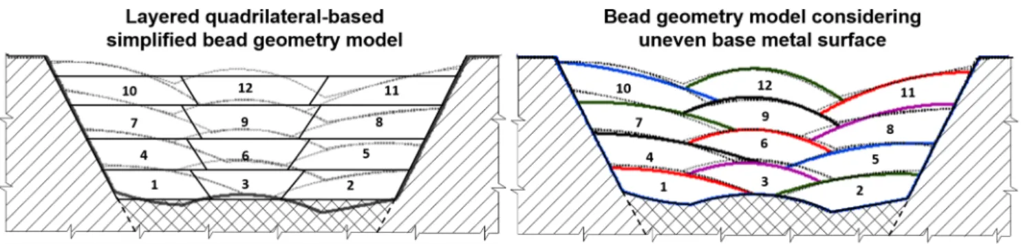
In small and medium-sized enterprises, during the small series production, the process’s tuning by trial and error method could take up a significant amount of time. In the planning phase, the beads are deposited layer-by-layer, and their shapes are usually simplified into quadrilaterals – reflecting only the bead size and position (Fig. 1).

However, a model describing the relationship between the process parameters and the resulting bead geometry can support selecting the process variables and the automated operation.

A wide range of bead shape models exists to describe a single bead based on the reviewed literature. Excluding those that produce a weld joint from a single bead, most of them are developed from bead-on-plate experiments, where the surface of the base metal plate is evenly flat due to machining. Even in those models applied in additive manufacturing or multi-pass welding, the quality of the base metal surface is neglected.

Even though, Li et al. (2018) showed that the base metal’s unsymmet- rical material distribution is influencing the fluid flow in the melted metal and, consequently, the weld’s shape bead after solidification. Still, no model was developed to describe a bead surface formation when deposited on uneven surfaces (Fig. 2). Our proposed model addresses this neglect by including the base metal surface quality besides the WPVs in our model as inputs.

In multi-pass welding one, an important factor is the amount of the deposited material, which can be calculated as A^d_Bcross-sectional area of the weld beads from the WPVs.

The theoretical A^d_Bcross-sectional area of the weld beads can be estimated according to Eq. (1) by calculating the amount of the deposited weld metal:

A^d_B=πD²_w 4 ⋅ vf

60vt

, (1)

where vf represents the wire feed rate, vt is the torch travel speed and Dw

is the feeding wire’s diameter. A η_ddeposition efficiency can be defined by comparing A^d_Bcalculated value with the measured bead area, given by the area under the bead surface curve on the given measured cross- section profile. According to (American Welding Society, 2001), the deposition efficiency is above 90 percent during TIG welding. However, the sign and the degree of the deviations might be inconsistent, causing error propagation in multi-pass welding as the layered beads are added on top of each other. The error is usually reduced on a given workpiece by on-site adjustment of the torch position and setting to constant the welding parameters across several layers.

Therefore, we expect that an accurate model utilizing the measurement data can increase the accuracy of the weld bead geometry accuracy. Computational intelligence techniques provide suitable tools to develop such a model. Based on our experience with the bacterial memetic algorithm (BMA) and its competitive performance with other Fig. 1. Traditional weld bead representation compared to the proposed method. (Left) The weld bead shapes are simplified into quadrilaterals and organized into layers. (Right) The weld bead shapes are described with a polynomial function and placed freely on the uneven base metal surface.

Fig. 2.Weld bead and its characteristics in a groove, deposited during multi- pass welding. The bead local coordinate system (LCS) is defined at the bead center.

(4)

techniques (Botzheim et al., 2009; Bal´azs, Botzheim, & K´oczy, 2010;

B´odis & Botzheim, 2018), we decided to utilize it and validate its applicability in multi-pass welding.

The objectives of the study are to (i) characterize the unevenness of the base metal surface, (ii) provide the estimation method of weld bead geometry formation on uneven surfaces, and (iii) apply the developed model on 304L stainless steel welding groove.

3. Proposed methods

Our proposed method introduces a modeling method of the weld bead profiles on uneven surface deposition and its application in multi- pass TIG welding. The method’s key components are the segmentation and characterization of the base metal surface and the modeling of the weld bead profile function. The base metal surface is handled in segments and approximated with a complete or incomplete second-order polynomial function. The bead profile model consists of fuzzy systems to estimate the coefficients of the bead shape function. The membership functions’ parameters are tuned by the bacterial memetic algorithm (Botzheim et al., 2009) during a supervised learning process and evaluated by the Mamdani inference model (Mamdani & Assilian, 1975).

3.1. Overview of the structure

In our method, we are utilizing the weld bead profiles measured by a laser triangulation sensor. The model can be applied even in sensor-less welding applications to estimate the weld bead shapes when deposited on an uneven base metal surface. The overview of the whole modeling and planning process is given in Fig. 3, and can be broken down into the

following steps:

Step 1. Acquisition and processing of the welding data, provided by the welding experiments and processed by the developed data processing framework (Section 3.2)

Step 2. Weld bead profile modeling by tuning the membership functions parameters of the fuzzy systems by BMA in order to infer the coefficients of the bead profile function from the welding process variables and the parameters of the base metal segments (Section 3.3)

Step 3. Application in Multi-pass welding of the developed bead model to estimate the bead profile shapes in the iterative bead placement process (Section 3.4)

Welding experiments were carried out on flat plates and in V-grooves to provide the measurement data to develop the empirical model (Sec- tion 3.2.1). The welding data were acquired in the form of measured profiles by a laser line triangulation sensor and the WPVs from the welding power source. Additionally, the position and orientation of the tool center were also recorded.

The measurements were aligned and synchronized in the measurement system to provide the organized data for the processing framework (Section 3.2.2). It was represented as weld bead cross sections in the perpendicular plane to the welding direction. Each bead processing took two profile scans of the cross-sections, one without and with the deposited bead. The analysis carried out in situ, the profile features were defined in the workpiece’s coordinate system. The final step of the data processing is the generation of the training data (Section 3.2.3) when the base metal- and the bead information is shifted into the weld bead’s Fig. 3.Overview of the proposed method’s structure. The main steps are: Aquisition and processing of the welding data (Step 1.), Weld bead profile modeling (Step 2.), and Application in Multi-pass welding (Step3.).

(5)

local coordinate system.

As the next step, the supervised training was performed by the BMA to realize the weld bead model (Section 3.3). The characteristic points of the trapezoidal membership functions of all rule bases were tuned to reduce the approximation error value (Ei in Fig. 3). The Ei defines the difference between the estimated and the desired value of the function coefficient in the i-th training pattern. All three coefficients of the bead shape function have their fuzzy system, and the bead shape function is given as a combination of them.

The application of the model is embedded in a welding process control system (Section 3.4). It is designed to be applied in a wide range of groove shapes; therefore, the workpiece is defined parametric, while the bead placement is a sequential process.

3.2. Acquisition and processing the welding data 3.2.1. Welding experiments

Bead-in-groove and bead-on-plate welding experiments were carried out to provide the empirical data for the modeling process. In both setup, 304L stainless steel with 40^◦C preheating temperature provided the base metal and 1.2mm diameter B¨ohler 13/4-IG wire the filler material. The experiments were executed in PA welding position, with a regulated constant 12V and 2.4mm arc gap. The E3 tungsten electrode’s diameter was chosen 3.2mm diameter to accommodate the arc current’s load.

Pure argon provided the shielding gas with a flow rate of 12− 14L/min.

The bead-on-plate experiments were carried out on a 20mm thick steel plate, clad welded 3mm deep with the filler material. The design of parameters followed an L25(5³) Taguchi design (Kacker, Lagergren, &

Filliben, 1991) layout with a few additional sets to replace the failed combinations. Welding failures happened in the design due to a non- optimal combination of WPVs, such as high heat input with a low wire feed rate or inadequate welding speed selection. Altogether, 33 different WPV combination were included, all of them with two inde- pendent trials on a 120mm length.

Bead-in-groove experiments were performed in straight V-grooves.

The edges of the 24.5mm thick and 390mm long workpieces were prepared with a 35^∘bevel angle, 2mm height root faces, and 1mm root gap. Three workpieces were involved in the process, each with a different bead layout containing between 28 and 35 beads.

In the verification process, the same preparation was made both for the flat plates and the welding grooves.

To record the weld bead profiles and the workpieces’ surface geometry, the M2DW 160/40 Line Laser Triangulation Sensor (LTS) was used. Each weld bead was measured by 0.1mm increments along the weld line, which supplied the raw data cross-sections for further data processing. The first and the last fifth of the weld beads were neglected;

thus, only the stabilized cross-sectional area was considered. The multi- pass welding experiments excluded the root pass since the welding

conditions are well defined and strictly controlled due to its critical impact on the final joint quality. The exported measurement data included – besides the profile points – the recorded tool center points and the actual values of the WPVs.

3.2.2. Profile segmentation and data processing

A framework was developed in LabVIEW^TMto process the bead profiles’ measurements, as the pseudo-code of the whole process is shown in Algorithm 1. The measurement data imported from the measurement system on the workpiece level, containing each weld bead and all the measured cross-sections.

Algorithm 1.: Processing of the bead profile measurements

The welding groove can be given in a CAD data file, a profile scan of the groove, or a combination of those two (Fig. 4). Additionally, the root path definition is also required to provide the robot trajectory reference points and the path normal-vectors. In each path point, the right-handed local coordinate system is defined by the normal-vector (directing towards the groove’s opening) as the y-axis and the vector directing towards the next path point as the z-axis. The characteristic cross-sections are defined at the path points in the x− y plane along the root path. The groove’s mathematical description is made for each characteristic cross- section from the digital representation of the workpiece.

The right-left part of the workpiece is considered according to the x- axis of the local coordinate systems, the positive x interval defines the right side, and the negative is the left. The segments’ describing functions are approximated by a second-order polynomial for unified description and a defined integral value in the coordinate system of x− y plane, where the x is the running variable. In a complex groove geometry, the groove slope function can be sectioned into several segments, described by elementary functions. In that case, the groove slope function became their superposed function, and the elementary functions should be used in their range of interpretation.

Upon loading the measurement data (Algorithm 1, ln.3), the individual cross-sections were merged into processible sections defined by the desired resolution along the weld line – 5mm thick sections in the recent application. The unified cross-sections were filtered by removing the measurement errors and applying a median filter of rank two and a second-order derivative filter. The unification of the cross-sections performed for each bead in the groove, therefore maintaining the profiles’ indexing. After the filtering, the base metal and the bead profiles are aligned, removing any remained distortion of the measurements and unification.

The next step in the process is the segmentation of the measured profiles (Algorithm 1, ln.6). First, the difference between the base metal and the bead profile is examined to locate the bead center’s approximated position and the toe points. Second, the main features are identified, such as the top surface of the workpiece, the groove faces, and the deposited beads’ uneven surface. Third, the individual beads and bead fractions are located according to the given number of visible bead Fig. 4. Digital representation of the welding groove including the root path and

a generated cross-section.

(6)

segments. The feature extraction is based on the first and second derivatives of the given profile points. It is approximated from the given points’ linear regression and its surrounding points in a given radius.

The profile points are then handled separately, and for each segment, the fitting curve is defined: linear fitting for the straight features and polynomial fitting for the bead segments. From that point, the profile is represented as a list of segmented features – each containing the type definition, the coefficients of the fitting curve, and the intersection point with the subsequent segment.

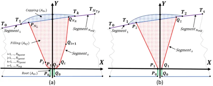
Fig. 5 illustrates a generalized, mathematical description of the groove geometry. Segments are defined between the groove features’

characteristic points – R points are on the top surface, P and Q points are located on the left and the right side of the groove, respectively. The NRpoint and NLpoint number of points are typically between two and four depending on the edge preparation. If the groove is a V-groove with a straight groove face, then there is no internal breakpoint; otherwise, the root radius (U-groove) and additionally, beveling defines more. Simi- larly, NTpoint defines the number of characteristic points on the top surface, thus the number of segments.

When all segments were identified, the bead characteristics are calculated (Algorithm 1, ln.8). The processing framework allows us to manually adjust the segment borders, which, after the confirmed mod- ifications, would update the whole segment list and the corresponding curve coefficients.

Fig. 2 depicts a general weld bead in a groove and the bead characteristics defined according to the image. These are namely: the area of the bead cross-section (AB), the coordinates of the bead center (BC), toe points (T1 and T2), and the contact angles at the toe points (Φ1 and Φ2).

The Si base metal segments are the earlier deposited bead surfaces or the groove edges. The points positions are given in mm in the Descartes coordinate system (in the workpiece coordinate system and the bead’s local coordinate system), the contact angles are in rad. The area of the weld bead is calculated as

AB=

∫_T

2

T1

fBdx− ∑^N^subs

i=1

∫_I_i

Ii−1

fSidx, (2)

where T1=I0 and T2=INsubs are the toe points (intersection points of the first and the last segments and the bead shape function, respectively), the points I1 to INsubs−1 are the intersection points of the adjacent segments, fB is the bead shape function, fSi is the shape function of the i-th segment. Both fB and fSi functions are given in the second order polynomial form

fB=B.a0+B.a1⋅x+B.a2⋅x² (3)

fSi=Si.a0+Si.a1⋅x+Si.a2⋅x² (4) The last step is post-processing (Algorithm 1, ln.11), when the whole bead is analyzed, and an overview is given about the bead characteristics features for each cross-section in graphical form. The system automati- cally detects if any of the evaluated characteristics are out of the acceptable range and marks the corresponding cross-section to be excluded from the export list. The range of acceptance is defined around the mean value of the given characteristics of the exportable cross- section.

Fig. 5. Definition of the characteristic points and the coordinate system on a (a) general groove and a (b) V-groove cross-section. Segments are defined between the characteristic points of the groove features – T points are on the top surface, P and Q points are located on the left and the right side of the groove.

Fig. 6. The inputs and outputs of the fuzzy systems as the key component of the weld bead shape model.

(7)

3.2.3. Generating training data for modeling

During the data export, besides the training data, the processed state of each cross-section is exported. Thus when the beads are re-evaluated, the already defined results are presented in the program. Furthermore, an overview is tabulated into a.csv file format to reference the training performance evaluation. The above-described process is carried out for each bead in the welding groove and all workpieces included in the model development.

The weld bead shape model is structured as multiple-input–single- output. The inputs are the four WPVs and the coefficients of the segment functions (Si.a0,Si.a1, and Si.a2), altogether 13 parameters. The outputs are the coefficients of the bead shape function (B.a0, B.a1, and B.a2) – each parameter is estimated by its fuzzy system (Fig. 6). Three WPVs were selected to be controlled to comply with the industrial aspect of the application, namely the arc current (I), the torch travel speed (vt), and the wire feed rate (vf). Additionally, as a recorded input value, the arc voltage (U) was also included because its small fluctuation still signifi- cantly affected the heat input. The parameter ranges are tabulated in Table 1, where the first column contains all the model’s inputs, and the second column the outputs. The bead shape coefficients are extended with the list of the bead’s characteristic parameters, where the ranges are interpreted for the measured values.

In the literature, several curvature descriptions are given to describe the shape function of the weld bead. However, the parabola shape was chosen because of its ability to characterize the segments generally in the welding groove. The bead profiles and straight lines can be given with only three parameters while a segment given with the root radius can be approximated with an acceptably small error.

The values of the ai coefficients in the parabola function, given as

a0+a1⋅x+a2⋅x², (5)

define the type of curve. If all ai coefficients are non-zero, then it is a general parabola, if only a1 =0, then it is a symmetrical one (the beads in the flat plate experiment described mostly like that). The case of a2= 0 describes a straight line, and if both a1 and a2 are zero, then it is a horizontal line, crossing the y-axis at a0. Such horizontal lines are describing the top surfaces of the grooves and the flat plates.

The segmented base metal, including all the groove’s visible features and the previously deposited beads, is represented as a list of coefficients of the segments, with the type definition and the intersection point’s x coordinate with the subsequent segment.

3.3. Bacterial memetic algorithm for training fuzzy systems

The weld bead shapes’ modeling is carried out utilizing fuzzy systems for the describing curve function’s coefficients. To define the fuzzy systems, the BMA was applied as a supervised trainer (Step 2. in Fig. 3) on the Npattern training patterns. The operations are carried out on the b bacterium, each encoding the fuzzy rules in their chromosomes (Botz- heim et al., 2009) as a b_kvector (k is the iteration variable of the individuals).

The rules in the fuzzy system are given in the following form:

Rulei: IFx1=Ai,1and … andxn=Ai,nTHENy=Bi,

where x= (x1,…xn)is the input vector, y is the output, Ai= (Ai,1…Ai,n) is the antecedent parameter vector, and Bi is the consequent parts in the i-th rule. The rule base is defined to cover the whole interval of inter- pretation of the input variables to provide a valid inference result.

Trapezoidal typed membership functions are used which can be written in the following form:

μ_A_ij(xj) =

⎧

⎪⎪

⎪⎨

⎪⎪

⎪⎩ xj− aij

bij− aij

, if aij<xj⩽bij

1, if bij<xj⩽cij

dij− xj

dij− cij

, if cij<xj⩽dij

0, otherwise

(6)

In this equation aij⩽bij⩽cij⩽dij denote the four breakpoints of the membership function belonging to the i-th rule and the j-th input variable. The output membership function in the i-th rule is also described as a trapezoid where the breakpoints are denoted as ai,bi,ci,di (Eq. (7)).

μ_B_i(y) =

⎧⎪

⎪⎪

⎪⎨

⎪⎪

⎩ y− ai

bi− ai

, if ai<y⩽bi

1, if bi<y⩽ci

di− y di− ci

, if ci<y⩽di

0, otherwise

(7)

As in the original Mamdani algorithm, the minimum operator is used as the t-norm in the inference mechanism, meaning that the degree of matching of the i-th rule in the case of an Ninput-dimensional crisp x input vector is:

Table 1

Ranges of the Parameters.

Input Name Notation Min value Max value units Output Name Notation Min value Max value units

Arc current I 180 260 [A] Bead a0 B.a0 0.5700 3.2426 [ − ]

Arc voltage U 11.3 13.9 [V] Bead a1 B.a1 −1.1876 1.1876 [ − ]

Torch travel speed vt 1.9 3.0 [mm/s] Bead a2 B.a2 −0.2983 0.10522 [ − ]

Wire feed rate vf 500 1900 [mm/min] Bead width w 5.1 13.6 [mm]

Segment-1 a0 S1.a0 −8.5490 2.3304 [ − ] Bead area AB 2.8 16.3 [mm²]

Segment-1 a1 S1.a1 −1.7163 0.41421 [ − ] Toe-1 X-coordinate T1.X −7.9 −1.3 [mm]

Segment-1 a2 S1.a2 −0.17121 0.16982 [ − ] Toe-1 Y-coordinate T1.Y −2.8 3.3 [mm]

Segment-2 a0 S2.a0 −0.18400 0.11662 [ − ] Toe-2 X-coordinate T2.X 1.3 7.9 [mm]

Segment-2 a1 S2.a1 −1.3061 1.3061 [ − ] Toe-2 Y-coordinate T2.Y −2.8 3.3 [mm]

Segment-2 a2 S2.a2 −0.38309 0.53976 [ − ] Contact angle-1 Φ1 1.0711 3.2035 [rad]

Segment-3 a0 S3.a0 −8.5491 2.3304 [ − ] Contact angle-2 Φ2 1.0711 3.2035 [rad]

Segment-3 a1 S3.a1 −0.41421 1.7163 [ − ] Segment-3 a2 S3.a2 −0.17121 0.16982 [ − ]

(8)

wi=min

Ninput

j=1μAij(xj). (8)

The output of the fuzzy inference is then:

The number of rules is Nrule, and Ninput is the number of input di- mensions.

By adjusting the breakpoints of the fuzzy rules’ trapezoids, the algorithm carries out the minimization of the E(b_k)cumulative error, defined as the 2-norm sum of squared ek error of the d^(p)desired and the

yk(b_k,x^(p))model’s output value. The output of the fuzzy rule bases is evaluated – in each step of the BMA and for all the bacteria – according to the Mamdani Inference Model for the x^(p)inputs as the p-th training pattern.

Algorithm 2.: Bacterial memetic algorithm y(x) =1

3

∑

Nrule i=1

3wi(d²_i− a²_i)(1− wi) +3w²_i(cidi− aibi) +w³_i(ci− di+ai− bi)(ci− di− ai+bi)

∑

Nrule i=1

2wi(di− ai) +w²_i(ci+ai− di− bi)

. (9)

(9)

E(bk) = ||ek||²₂ (10) ek= [e^(p)_k ] = [d^(p)− yk(bk,x^(p))] (11)

Algorithm 2 shows the pseudo-code of the BMA and in Table 2 the applied meta parameters are listed. The BMA consists of three main calculation steps: the Bacterial mutation, the Local search, and the Gene transfer. The iterative process is performed the number of generations (Ngen) times, starting with an initial population containing Nind random individuals applying the predefined (Nrule) number of rules. Thus, in the initial population creation, the total number of the created membership functions is Nind⋅(Ninput+1)⋅Nrule where Ninput=13 is the number of input variables and each membership function has four parameters to main- tain their trapezoidal characteristics.

In each generation, the Bacterial mutation and the Local search are applied to each individual, and the Gene transfer on the whole population at once.

3.3.1. Bacterial mutation

In the Bacterial mutation step, the bacteria and its Nclone clones are subjects of random changes in their genes, which according to the Munit

mutation unit can either be a point (breakpoint of the trapezoid), a membership function (trapezoidal, four points), or an entire rule. In each iteration, Nclone clones are created then the random changes are performed. The number of modified genes is given by the lbm mutation segment length. After that, all the clones are evaluated, the best clone transfers the mutated part into the other clones, and in the end, only the best rule base is kept. The Bacterial mutation is repeated Nsegment times, where

Nsegment=4⋅Nrule⋅(Ninput+1)/

lbm (12)

in the case when point mutation is applied (Munit is set to point).

3.3.2. Levenberg–Marquardt algorithm

The Local search in BMA was utilizing the Levenberg–Marquardt algorithm and carried out with a LMprob probability for each individual until the complex τ_k<τ (Botzheim et al., 2009) terminal condition is

met or the maximum LMiter number of iteration steps is reached.

Let denote J(bk)the Jacobian matrix of bacterium bk: J(bk) =

[∂yk(bk,x^(p))

∂b^T_k ]

, (13)

where each row of the J(bk)matrix contains the partial derivatives of the bacterium bk encoded fuzzy system’s output calculated for the given x^(p) input training pattern. The detailed definitions of the derivatives and the calculation steps are given in Botzheim et al., 2009.

In the Levenberg–Marquardt algorithm, the approximation towards the local minimum is defined by the sk update vector, rk trust region, and γ_kbravery factor.

sk= − (J^T(bk)J(bk) +γ_kI)⁻¹J^T(bk)ek, (14) rk= E(bk) − E(bk+sk)

E(bk) − ||J(bk)sk+ek||²₂ (15)

The value of γ_kbravery factor controls both the search direction and the magnitude of the update – adjusted dynamically depending on the value of the rk trust region. If the value of γ_kconverges towards zero, then the algorithm applies the Gauss–Newton method; if towards infinite, the algorithm gives the steepest descent approach.

γ_k+1=

⎧⎨

⎩

4⋅γ_k if rk<0.25 γ_k/2 if rk>0.75 γ_k otherwise

(16)

The local search is evaluated as successful if the update vector modifies the bacterium towards the local minimum. In this case, the bacterium’s new value is carried on; otherwise, it is left unchanged.

bk+1=

{bk+sk if E(bk+sk)<E(bk)

bk otherwise (17)

3.3.3. Gene transfer

The last operation in a generation is the horizontal Gene transfer, allowing the recombination of genetic information between two bacteria. This operation is performed Ninf number of infection times per generation. The individuals are organized into ascending order according to their E error value then split into halves representing the better and the worse individuals. During the infection, a randomly chosen, better bacteria overwrites a randomly chosen, worse one’s gene with its own Iunit infection unit time lgt infection segment length. The infection unit here may be defined in the same ways as the Munit mutation unit. When the Gene transfer operation is finished, the new generation’s execution starts until the predefined number of generations (Ngen) is performed.

3.4. Application in multi-pass bead positioning

During the application of the developed bead shape estimation model, an iterative process is carried out to place the weld beads in the welding groove sequentially. The pseudo-code of this placement process is presented in Algorithm 3. The operation requires the description of the welding groove (according to Section 3.2.2) and the Welding Plan, containing the information about the WPVs and the tool center point (TCP) for each Nbead weld bead. If the welding plan were the desired output, the additional rules of bead positioning and WPVs selection would be necessary, which requires further discussion but not part of this article.

Table 2

Parameters of the BMA

Parameter Name Notation Value

Number of inputs Ninput 13

Number of patterns Npattern 5458

Number of rules Nrule 2 – 12

Number of generations Ngen 50

Number of individuals Nind 50

Number of clones Nclone 3

Mutation unit Munit point

Mutation segment length lbm 1

Probability of LM¹ LMprob 40

Max. LM iteration step LMiter 8

Bravery factor (initial) γ_init 1.00

Terminal condition τ _0.0001

Number of infections Ninf 50

Infection unit Iunit rule

Infection segment length lgt 1

1Levenberg–Marquardt algorithm

(10)

For simplicity, we assume that the Welding Plan is available.

Algorithm 3.: Model application in multi-pass welding

In the initialization, the Groove description provides the initial list of the segments. The process starts with the acquisition of the BeadCenter, defined as the intersection of the center-line of the welding torch (going through the TCP) and the base metal’s surface. Based on the given bead center, the list of the probably SegmentCombinations can be selected since there is no information about how wide the weld bead will be; thus, it can stretch over multiple segments or remain within one segment’s borders.

Since three adjacent segments need to be entered, the proper combination should be selected (Algorithm 3, ln 4.), as shown in Table 3.

One segment (index 0) is fixed as it contains the bead center, but the two sides need some consideration. As the most common scenario, the pre- vious and the following segments are selected (case 0). If the bead is too small, or the given base metal segment is large, the two sides would be the same as the middle segment (case 1). On the other hand, the bead can be deposited asymmetrically like one side is still on the center’s segment, and the other one is on an adjacent segment (cases 2 and 3). In the unlikely event that the adjacent bead is small, the bead’s side would stretch over the second segment (cases 4 and 5).

The Segment Combinations with the WPVs can be entered into the previously developed model to acquire the B.a0,B.a1,B.a2 coefficients of the bead surface function.

When the bead model is applied and fed with the segment information, all the cases mentioned earlier are given, then the resulting bead shape is evaluated (Algorithm 3, ln 8.). The cases fulfilling the criteria that the segments’ index containing the toe points match the fed segments’ indices are kept the other cases are neglected. If multiple satis- factory combinations are found, the priority is given to those which toe points are closer to the Bead Center and covering an area with less difference to the expected bead area.

The characteristics of the newly acquired bead can be evaluated now.

The exact shape allows us to perform manufacturing-critical analysis of the process and highlight the bead’s problematic locations, thus elimi- nating the welding defects. A good measure is to monitor the Φ₁and Φ₁ contact angle values. If a too-narrow gap is created, the fusion could be incomplete, gas pockets or slag inclusions could appear.

In the last step of the planning process (Algorithm 3, ln 10.), when

the new bead is defined, the segment list is updated to include it and remove the fully covered segments or those whose remaining length became neglectable. The iterations are repeated until all weld bead is deposited.

4. Results and discussion

In the following, the development work results will be discussed, including the overview of the main findings of the modeling process of the weld bead profiles. The performance of the development model was compared with a statistical model (multi regression analysis, MRA) models, and over cross-validation, too. Furthermore, demonstration and evaluation of the application cases are presented.

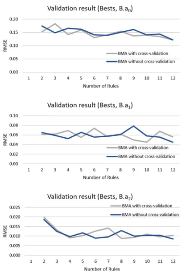
The trained model’s performance was evaluated by comparing the estimated and the measured values to define the goodness of the fitting using the root mean square error (RMSE). The RMSE values were given for the bead geometry with the bead shape function defined by the estimated coefficients and compared with the measurements. Beside the direct comparison of the B.a0,B.a1, and B.a2 coefficients; the calculated values of the AB bead area, w bead width, location of the T1 and T2 toe points and the three-phase contact angle (Φ) values were considered.

The value of the toe points’ positioning error is calculated as the distance between the estimated and the measured locations. Similar comparisons were carried out for a separate set of validation data.

The data sets for the training and validation were extracted from the welding experiments. The processing of the cross-sections of the weld beads and the base metal provided the patterns. The patterns were generated two ways for each cross-section since they could be seen from two views – a straight view and a mirrored one. Therefore, the double amount of pattern could be used in the model’s tuning because the segments’ descriptions were not symmetric, thus containing additional information for the model. The mirrored pattern generation required to negate the value of the a1 coefficients of each function (both the base metal’s and the bead’s), then swapping all coefficients’ position of Segment–1 and Segment–3. The WPVs of the pattern was left unmodified.

The mirroring was only necessary to be performed on the patterns generated from the cross-sections of beads deposited in the welding groove.

One of the mirrored views of the three workpieces was selected as validation data. The fitting evaluation was carried out on each bead and cross-section individually, the multi-pass validation on the whole filled groove. Altogether, 5458 different bead cross-section was used during the training and 947 bead cross-section in the validation data set.

During the data processing, some of the bead cross-section failed to be processed and distorted the later results. Therefore, a filter was applied, based on the expected bead area, as discussed in Section 2. The deposition efficiency may vary depending on the WPVs, but while filtering the measurement and estimation data, the lossless value is set as the reference deposited cross-sectional area. Both the measured and estimated data were filtered according to the deviation from the reference area, where the threshold set to arbitrary ±0.3. The wide threshold range was chosen only to remove the clearly outlying data points. Over the set threshold limit, the data point was considered faulty due to some unforeseen errors in the processing system. This filtering method can also be used during the model’s application since the WPVs values are typically defined beforehand.

4.1. Multiple regression analysis model

Multiple regression analysis was performed to create a reference model to our method since no similar model exists in the overviewed literature. The regression model data sets were the same as were used for training and validating our machine learning models. The extracted regression coefficients for coefficients of the bead shape function are tabulated in Table 5. The coefficients with the significant effect (level of significance is p≤0.05) on the modeled output were marked with an Table 3

Possible selection of the segment from the base metal segment list (index 0 is the segment containing the bead center)

Case Segment–1 Segment–2 Segment–3

0 −1 0 +1

1 0 0 0

2 −1 0 0

3 0 0 +1

4 −2 − 1 0

5 0 +1 +2

(11)

asterisk, next to the p-value. Since each input parameter has a significant effect on at least one output parameter, none of them can be excluded from the modeling. The coefficient of determination (R²) as calculated for each output parameter are: 0.889 for B.a0,0.793 for B.a1, and 0.677 for B.a2.

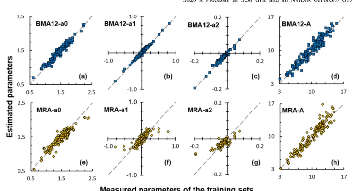
The calculated RMSE values for the training and validation are presented in the first row of Table 4.. The goodness of fitting is visualized in Fig. 7 with yellow rhomboid markers by plotting the comparison of

the estimated and the measured coefficients, and additionally, the bead cross-sectional area. Both in the training and the validation, the MRA model provided a sufficient fitting for the data, verifying the data set’s coherency. However, the best performing BMA trained fuzzy system (marked by blue squares) outperforms the MRA model during the validation. Furthermore, as shown later, most of the examined model by BMA would have better fittings than the MRA model.

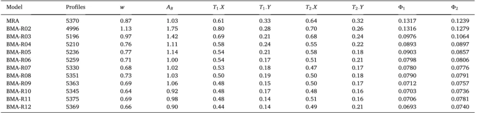
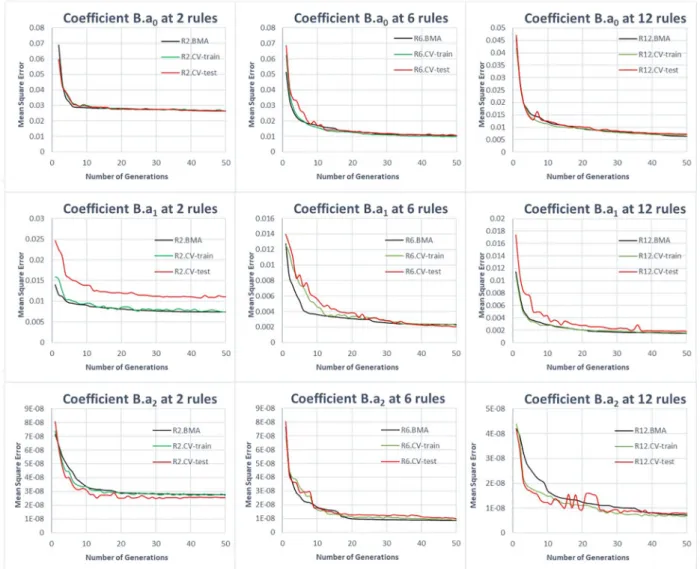
4.2. Evaluation of the trained fuzzy systems

The fuzzy systems were trained with a different number of rules, set between two and twelve. The required calculation time depended on the number of rules since they defined the number of segments in the bacteria’s chromosomes (see Eq. 12). In the case of two rules, the number of segments is 112, while for twelve rules, it is 672. The computations of the fuzzy systems were carried out on a PC using an Intel® Core™ i7- 5820 K Processor at 3.30 GHz and an NVIDIA GeForce® GTX 970

Table 5

MRA model coefficients to estimate the B.a0,B.a2, and B.a2 coefficients of the weld bead function.

B.a0 B.a1 B.a2

Name Coefficient p-value Coefficient p-value Coefficient p-value

Intercept 2.6193 0.0000 * 0.0032 0.9793 -0.1501 0.0000 *

Arc current -0.0031 0.0000 * 0.0002 0.1722 0.0004 0.0000 *

Arc voltage -0.0941 0.0000 * 0.0019 0.8537 0.0042 0.0756

Torch travel speed -0.2585 0.0000 * -0.0209 0.0211 * -0.0053 0.0112 *

Wire feed rate 0.0009 0.0000 * 0.0000 0.2037 0.0000 0.0000 *

Segment-1 a0 0.1442 0.0000 * -0.0424 0.0000 * 0.0062 0.0000 *

Segment-1 a1 -0.4189 0.0000 * 0.2140 0.0000 * -0.0309 0.0000 *

Segment-1 a2 0.0625 0.5926 1.1911 0.0000 * -0.0596 0.0040 *

Segment-2 a0 -0.1954 0.1033 0.0728 0.4275 0.5881 0.0000 *

Segment-2 a1 -0.0086 0.3811 0.2592 0.0000 * 0.0074 0.0000 *

Segment-2 a2 -0.1260 0.0242 * 0.0090 0.8330 0.3161 0.0000 *

Segment-3 a0 0.1540 0.0000 * 0.0401 0.0000 * 0.0076 0.0000 *

Segment-3 a1 0.4449 0.0000 * 0.2066 0.0000 * 0.0299 0.0000 *

Segment-3 a2 -0.5144 0.0000 * -1.1732 0.0000 * -0.1109 0.0000 *

Fig. 7.Fitting plots of the estimated and measured coefficients of the bead shape function and bead area. (a) – (d) parameters estimated by the BMA model utilizing 12 fuzzy rules for the training data, (e) – (h) parameters estimated by the MRA model for the training data.

Table 4

RMSE values of the MRA model for the training and the validation.

RMSE B.a0 B.a1 B.a2

Training 0.1122 0.0858 0.0194

Validation 0.2171 0.1791 0.0217